COMBINED DETAILED AND QUASI STEADY-STATE TIME SIMULATIONS
FOR LARGE-DISTURBANCE ANALYSIS
Thierry Van Cutsem Marie-Eve Grenier, Daniel Lefebvre
FNRS and University of Li`ege Hydro-Qu´ebec, TransEnergie division
Li`ege, Belgium Montr´eal, Canada
t.vancutsem@ulg.ac.be lefebvre.daniel.4@hydro.qc.ca
Abstract - This paper deals with the simulation of long-term power system responses to large distur-bances in the presence of discrete events. A method combining detailed and quasi steady-state time simula-tions is presented, the former being used for accuracy and the latter for efficiency reasons. Detailed time sim-ulation is used to analyze the short-term period follow-ing a large disturbance and identify the discrete con-trols triggered. Next, quasi steady-state simulation is used to simulate the same time interval with the dis-crete controls imposed as external events, before letting the system evolve as usual in the long term. This sim-ple method has been successfully tested on the Hydro-Qu´ebec system.
Keywords - long-term dynamics, time domain sim-ulation, quasi steady-state approximation, voltage stability, frequency dynamics
1 INTRODUCTION
I
N power system dynamic studies, the trend is to perform numerical simulations over longer periods of time, with more detailed models, and for more op-erating conditions and disturbances. However, power system dynamic models are large and involve very different time scales, which makes their simulation over long time intervals very demanding.To deal with this complexity, variable step size simulation tools have been devised [1]. Nevertheless, many companies use software relying on fixed time step algorithms and do not envisage to change their simulation environment.
An alternative consists in combining detailed and simplified simulation tools [2, 3]. The former is used over a time interval following the disturbance, where large transients are caused by the faster dynamics. If the system has survived this period, and once these transients have died out, a simpler model is used in which the faster dynamics are neglected.
The idea of time-scale simplification of a model is not new. It underlies the quasi-sinusoidal (or pha-sor) approximation used in most stability studies [4],
where electromagnetic transients are neglected and the network is modeled by algebraic equations. The idea is further exploited in the Quasi Steady-State (QSS) approximation of long-term dynamics, which consists of replacing the short-term differential equa-tions of generators, motors, compensators, etc. by the corresponding algebraic equilibrium equations [6]. QSS simulation is well suited to computationally in-tensive tasks such as security limit determination, real-time applications or training simulators [5, 6, 7]. When combining the detailed and QSS models, however, it is essential to both preserve the reliability of the overall simulation and make the combination of tools totally transparent to the end-user.
A time-scale decomposition-based simulation tool of the type outlined above was already proposed in [2] and has been used for several years by Hydro-Qu´ebec (H-Q) engineers. Within the context of the H-Q migration to another detailed simulation tool, the method has been revisited and a new, easier to implement scheme has been devised.
This paper is organized as follows. Section II states the problem while Section III presents the new approach. Section IV reports on results obtained on the H-Q system. Conclusion and perspectives are of-fered in Section V.
2 STATEMENT OF THE PROBLEM 2.1 System modeling
In stability studies, the general dynamic model of a power system takes on the form:
0 = g(x, y, zk) (1)
˙
x = f (x, y, zk) (2)
zk+1 = h(x, y, zk) (3)
The algebraic equations (1) relate to the network. The differential equations (2) relate to a wide va-riety of phenomena and controls including:
• the short-term dynamics of generators, tur-bines, governors, Automatic Voltage
Regula-tors (AVRs), Static Var CompensaRegula-tors (SVCs), induction motors, HVDC links, etc.
• the long-term dynamics of secondary fre-quency and voltage control, load self-restoration, etc.
Finally, the discrete-time equations (3) capture discrete events that stem from:
• controllers acting with various delays on shunt compensation, generator setpoints, Load Tap Changers (LTCs), etc.
• equipment protections such as OverExcitation Limiters (OELs), etc.
• system protection schemes against short and long-term instabilities, acting on loads and/or generators.
It must be emphasized that, apart from digital con-trollers operating at constant sampling rate, the dis-crete events take place at time instants dictated by the system dynamics itself (which is not captured by the notation).
In the above equations, y is the vector of bus volt-ages while x (resp. zk) is the vector of continuous
(resp. discrete) states.
In the sequel, the numerical integration of the whole model (1-3) is referred to as Full Time-Scale (FTS) simulation.
2.2 Principle of the QSS approximation
As indicated previously, the QSS approximation of long-term dynamics consists of representing faster phenomena by their equilibrium conditions instead of their full dynamics. The correspondingly simplified model takes on the form:
0 = g(x1, x2, y, zk) (4)
0 = f1(x1, x2, y, zk) (5)
˙
x2 = f2(x1, x2, y, zk) (6)
zk+1 = h(x1, x2, y, zk) (7)
in which x (resp. f) has been decomposed into x1
and x2 (resp. f1and f2).
In long-term voltage stability studies, the short-term dynamics of generators, turbines and excitation systems can be neglected. Furthermore, (5) may take on the form of three algebraic equations per machine [5, 6]. The latter account for saturation, AVR voltage droop and governor speed droop effects. Frequency is a component of x1.
If frequency dynamics is of interest, a simplified turbine and governor representation can be retained in (6). Assuming the same speed for all generators and accounting for their inertia, the rate of change
of frequency provides an additional equation (6) [8]. Frequency is then a component of x2.
2.3 Limitation of the QSS approximation
The QSS approximation is appropriate for check-ing voltage security with respect to “normal” (typ-ically N-1) contingencies [5, 7]. When dealing with severe disturbances, expectedly, the QSS model meets some limitations.
The first limitation lies in the implicit assump-tion that the neglected short-term dynamics are sta-ble. After a large disturbance, the system may loose stability in the shortterm time frame (within say -the first 10 seconds after -the disturbance) and hence not enter in the long-term phase simulated under the QSS approximation.
The second limitation is linked to the discrete events represented by (3). A large disturbance may trigger controls with great impact on the system long-term evolution (e.g. shunt compensation switching, underfrequency or undervoltage load shedding, etc.). As already quoted, the sequence of controls depend on the continuous dynamics, and hence may not be correctly identified from the simplified QSS model. 2.4 Combining detailed and QSS simulations
The objective of coupling detailed and QSS sim-ulations is to combine the reliability of the former, when dealing with the short-term dynamics, with the efficiency of the latter, when simulating the long-term dynamics.
A first approach was proposed in [2]. In the lat-ter, the detailed model (1-3) is used to analyze the short-term period following a contingency, and once the corresponding dynamics have died out, switching to the QSS model takes place. The state variables of the QSS simulation have to be initialized from the final system state provided by the detailed simula-tion. Hence, the latter does not start from the steady state provided by a load flow program, as in con-ventional time simulations, but rather “out of equi-librium”. This initialization procedure has to be im-plemented in the detailed simulation tool, which can be considered as a constraint. Furthermore, the ini-tialization is more delicate when frequency dynam-ics are included in the QSS model, which was not the case in [2].
The new approach described in the remaining of the paper is free from these drawbacks, since the cou-pling is performed by post-processing the results of the detailed simulation.
3 THE PROPOSED METHOD
The proposed method consists of the following steps, where the disturbance of concern is applied at t = 0 and the system response is sought for t ∈[0 tf in]:
1. run a detailed simulation over the short-term interval [0 tsw]. If the system is unstable, stop;
2. otherwise, identify the discrete events that have occurred over this interval;
3. run a QSS simulation on the same interval, im-posing those events as “external disturbances” while preventing the corresponding discrete devices to act by themselves;
4. proceed with the remaining of the QSS simu-lation, over the ]tsw tf in]interval with the
au-tomatic devices free to act as usual.
This procedure is justified as follows. Shortly after t = 0, the short-term dynamics responds to the disturbance with large transients. The full model (1-3) must be used to check system stability and iden-tify the sequence of discrete events. The latter may not be correctly identified from the QSS model (4-7). However, by imposing the right sequence iden-tified from the detailed model, the QSS system re-sponse on [0 tsw] is improved and, once the fast
transients become small enough, both responses are likely to be close to each other. From there on, the QSS model is a better approximation of the full one and the sequence of discrete controls can be deter-mined on ]tswtf in]with reasonable accuracy.
Let us now illustrate how the discrete events are handled at steps 3 and 4 of the procedure, with a sim-ple logic present in many controllers. The latter con-sists in comparing a quantity y to a threshold value ymin and taking an action (e.g. switching
compen-sation, shedding load, etc.) if y < ymin for some
duration τ.
Consider for instance the situation depicted in Fig. 1. The controller starts its timer at t = to and
should act at t = t1, where t1 −to = τ. At step 3
of the procedure, however, the controller is “frozen” and does not act. Instead, the action is imposed at a time t2identified from detailed time simulation (step
2). In the shown example, the effect of this action is to bring back y above ymin, which stops the timer.
Note that if t2 was smaller than t1, the action would
nevertheless be imposed at t = t2.
At t = tsw, the simulation enters step 4 and the
controllers are “freed”. Carrying on with the same example, if y falls again below ymin at t = t3, the
controller acts as usual at t4= t3+ τ since this time
is larger than tsw. QSS simulation y t ymin to t1 t2 t3 t4 τ τ step 3 step 4 tsw 0
Figure 1: handling of discrete events
As regards the choice of tsw, it should be as
small as possible to shorten the whole computing time but large enough to guarantee the reliability of the combined simulation. More precisely, it should be large enough to ascertain the short-term stabil-ity of the system and correctly identify the discrete events trigerred by the short-term dynamics. This choice is further illustrated in the next section.
4 RESULTS
4.1 The Hydro-Qu´ebec system and its model With its long 735-kV transmission corridors be-tween the hydro generation areas in the North and the main load centers in the South part of the province, and its isolated mode of operation, the H-Q system is exposed to angle, frequency and voltage stability problems.
Besides static var compensators and synchronous condensers, the automatic shunt reactor switching devices - named MAIS - play an important role in voltage control [9]. These devices, in operation since early 1997, are now available in twenty-two 735-kV substations and control a large part of the total 25,500 Mvar shunt compensation. Each MAIS device relies on the local voltage, the coordination between sub-stations being performed through the switching de-lays. While fast-acting MAIS can improve transient angle stability, slower MAIS significantly contribute to voltage stability. MAIS devices react to voltage drops but also prevent overvoltages by reconnecting shunt reactors when needed.
Voltage stability is a concern near the load cen-ters of Montr´eal and Qu´ebec city. Long-term voltage stability studies are routinely performed at Hydro-Qu´ebec using detailed simulation, QSS simulation and the combination of both. The contingencies of concern are the tripping of 735-kV transmission
lines, especially those feeding the southern part of the system.
The system model includes 846 buses and 132 generators. The discrete events stem from: 371 LTCs acting at different voltage levels with various delays, 89 MAIS devices, 9 OELs protecting the synchro-nous condensers located near the main load areas, 9 (instantaneous) admittance limiters acting on the SVCs. Fourty-five MAIS react to voltage drops, with thresholds ranging from 0.95 to 0.97 pu and switch-ing delays from 0.7 to 20 seconds.
4.2 Implementation of the combined simulation As regards Step 1 of the proposed method, the simulation stops when no MAIS device has been trigerred over the last 10 seconds of simulated time. This indeed indicates that the short-term dynam-ics have died out sufficiently, while 10 seconds are enough to detect short-term instability.
As regards the QSS simulation part, the reactor switchings by MAIS devices are discrete events that must be treated as described in Section 3 and Fig. 1, i.e. imposed at Step 3 of the procedure and freed at Step 4. LTCs are treated in the same way, for accu-racy reasons. On the other hand, results have shown that OELs and SVC limiters can be left to act as usual during the QSS simulation.
Figure 2 sketches how the coupling is imple-mented. The ST600 software of H-Q is used for de-tailed simulation. An interface (hq2ulg) translates the load flow data and extracts the subset of dynamic data relevant to QSS simulation. The latter is per-formed by the ASTRE software developed at the Uni-versity of Li`ege. This procedure has been in use for several years for voltage security assessment against N-1 contingencies [5]. The part shown with dotted lines in Fig. 2 relates to the combined simulation. Namely, ST600 produces a log file with the sequence of discrete events. This ASCII file is read by a small utility (csa) which translates the events into external disturbances to be imposed in the QSS simulation.
Obviously, all these steps are totally transparent to the user. In particular the detailed and QSS sim-ulation plots are assembled as if they were produced by a single tool.
As can be seen, the coupling is simple and can accommodate various detailed simulation softwares, the csa utility being adjusted accordingly. A simi-lar procedure is being devised to couple ASTRE with PTI’s PSS/E. data dynamic csa ASTRE hq2ulg ST600 events discrete QSS data data load flow
Figure 2: implementation of the combined simulation
4.3 QSS vs FTS simulation
The purpose of this section is to illustrate how the QSS model (4-7) approximates the full model (1-3), before reporting on the proposed method.
Figures 3 to 5 deal with the system response to an N-1 contingency, computed under various condi-tions. The incident is the tripping at t = 1 of a major 735-kV line of the H-Q system. All the plots of this section show the time evolution of the voltage at the receiving end of the line, located near Montr´eal. The pre-contingency voltage is 1 pu.
The solid line in Fig. 3 relates to the FTS simula-tion. The latter uses a time step of 0.0083 s (a half-cycle at 60 Hz). Three reactors (of 330-Mvar each) are tripped by MAIS at t = 35.9, 93.2 and 190.4, re-spectively, as can be seen from the voltage spikes in the figure. The voltage oscillations are caused by the long-term frequency dynamics.
0.97 0.975 0.98 0.985 0 50 100 150 200 250 t (s) V (pu) FTS simulation QSS simulation with discrete events imposed
Figure 3: Effect of neglecting short-term dynamics
The dotted line in the same figure relates to a QSS simulation in which all MAIS and LTCs have been frozen for the whole simulation while the cor-responding shunt admittances and transformer ratios are forced to change as identified in the FTS simula-tion. Clearly, there is no gain in computing time to be
expected from such a simulation (since FTS is used over the whole time interval); the objective is rather to assess the impact of the QSS approximation. In-deed, the difference between the two simulations is only due to the replacement of Eq. (2) by Eqs. (5,6), the discrete changes being the exact ones. As can be seen, the QSS evolution is a very good approxima-tion of the FTS one, although it is 100 to 1000 times faster (as confirmed by the results of Section 4.6).
In Fig. 4, the same FTS simulation is compared to a “traditional” QSS simulation in which the MAIS and LTC changes are decided by the QSS system evo-lution itself. As can be seen, the two responses dif-fer mainly by the times at which the last two shunt reactors are tripped. This difference is due to short-term transients. For instance, in the FTS simulation, the voltage spike at t = 35.9 resets some LTCs (the controlled voltages re-entering the deadbands tran-siently) and delays their reaction. Since the voltage spike is not present in the QSS response, the LTCs move earlier in the QSS simulation, which causes the voltage to drop and, hence, the second MAIS to be triggered earlier as well.
0.97 0.975 0.98 0.985 0 50 100 150 200 250 t (s) V (pu) FTS simulation QSS simulation Figure 4: FTS vs QSS simulation
Nevertheless, the QSS output is quite acceptable for this N-1 contingency, since it leads to the right number of shunt reactor trippings and the same final voltage. In fact, the switching times are not consid-ered critical by H-Q engineers (even the full model relies on simplifications ! These uncertainties are compensated by the closed-loop nature of the MAIS controls). More attention is paid to the number and location of trippings, although a discrepancy by one shunt reactor is still accepted. However, the discrep-ancy could be larger when the system is subject to a more severe disturbance, which is one motivation for the method presented in this paper.
Figure 5 shows the effect of incorporating fre-quency dynamics to the QSS model. The QSS evo-lution with (resp. without) this dynamics is shown with solid (resp. dotted) line and has been computed with a time step of 0.1 s (resp. 1 s). The two curves do not differ very much. The voltage response is a little more accurate when accounting for frequency effects, although this gain does not by itself justify the use of the more refined model, whose comput-ing time is 5 to 10 times longer (although still very short) [8]. Further investigations are needed to im-prove the QSS model in this respect. Note finally that impedances are updated with frequency in the FTS simulation, while they are kept constant in the QSS one. 0.97 0.975 0.98 0.985 0 50 100 150 200 250 t (s) V (pu)
QSS simulation with frequency dynamics QSS simulation without frequency dynamics
Figure 5: Effect of frequency model in QSS simulation
4.4 A detailed coupling example
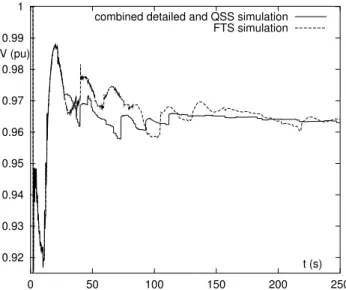
An example of coupling by the proposed method is given in Fig. 6 where the solid curve relates to the combined simulation and the dotted one to FTS sim-ulation, for comparison purposes. The disturbance of concern is a double line tripping applied at t = 1.
Using the above mentioned criterion, the detailed simulation stops at tsw = 25. Over the same 25
sec-onds, a QSS simulation is run with the MAIS and LTC controls frozen, while changes in 6 shunt ad-mittances and 46 transformer ratios are imposed at the various times identified by detailed simulation. The corresponding system evolution is normally not shown to the user, since detailed simulation results are available. This is why a single curve is shown for t ∈[0 25]in Fig. 6.
At t = 25, these controls are released, i.e. they become free to act as usual. The QSS simulation pro-ceeds for 225 s. The corresponding evolution some-what departs from the FTS reference, for already
mentioned reasons, but the overall accuracy is good and the system evolution is correctly declared stable.
0.92 0.93 0.94 0.95 0.96 0.97 0.98 0.99 1 0 50 100 150 200 250 t (s) V (pu)
combined detailed and QSS simulation FTS simulation
Figure 6: example of coupling
Table 1 details the time and location of shunt reactor trippings in the FTS and combined simula-tions, respectively. As in the previous example, most switchings take place earlier in the QSS simulation but their number and locations are the same.
FTS combined at t = bus # at t = bus # 4.0 714 step 3 11.3 715 same as FTS 12.3 702 t ∈[0 25] 13.3 701 14.3 707 40.5 708 43.1 708 step 4 59.4 703 47.1 703 106.7 730 77.1 730 t ∈]25 250] 131.9 704 98.7 704 189.3 713 123.3 713
Table 1: sequence of shunt trippings
4.5 Accuracy of security limit determination The most appropriate way of checking the accu-racy of the proposed method is by computing security margins, which is its main purpose. For a given set of sources and sinks, the secure operation margin is defined as the maximum power transfer increase that still results in a stable post-disturbance evolution [5]-[7]. A load flow is used to obtain the pre-contingency states and a binary search to determine a stable and an unstable value of the power transfer that differ by less than a tolerance. The latter is set to 100 MW.
The margins have been checked on a representa-tive set of 5 scenarios described in Table 2, where the number of switched reactors refers to the marginally
stable case.
cont. severity pre-disturb. Nb of switched
# configuration reactors 1 N-2 intact 5 2 N-2 2 lines out 10 3 N-2 intact 19 4 N-2 intact 3 5 N-1 2 lines out 3
Table 2: contingency description
For each contingency, Table 3 provides the last stable and the first unstable power increase. The power margins given by the proposed and FTS sim-ulations do not differ by more than 100 MW, which is quite accurate for the H-Q system. Furthermore, in terms of tripped reactors, the discrepancy between the proposed and the FTS simulations is zero in al-most all cases and never exceeds one, which meets the H-Q criteria.
FTS combined
cont. marginally marginally
# stable unstable stable unstable
1 300 400 400 500
2 400 500 400 500
3 1400 1500 1400 1500
4 2400 2500 2400 2500
5 1600 1700 1500 1600
Table 3: last stable and first unstable power increases (in MW)
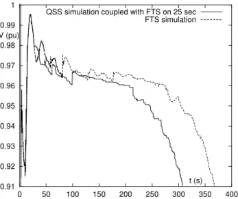
Figures 7 and 8 compare the voltage evolu-tions provided by the combined and FTS methods in the marginally stable and unstable cases of contin-gency 2, respectively. This comparison is demand-ing since near the stability limit, small changes may later result in large deviations of the system evolu-tion. Nevertheless, the combined simulation reliably fits the FTS one.
0.92 0.93 0.94 0.95 0.96 0.97 0.98 0.99 1 0 50 100 150 200 250 t (s) V (pu)
combined detailed and QSS simulation FTS simulation
0.91 0.92 0.93 0.94 0.95 0.96 0.97 0.98 0.99 1 0 50 100 150 200 250 300 350 400 t (s) V (pu)
QSS simulation coupled with FTS on 25 sec FTS simulation
Figure 8: Simulation of marginally unstable case
4.6 Computational efficiency
Table 4 gives the computing times of six repre-sentative simulations, by the FTS and the proposed methods. For the latter, results are shown as sums of detailed and QSS simulation times. All these times include data reading and have been measured on a 2.2-GHz PC. As can be seen, the proposed method is 4.9 to 8.2 times faster than FTS simulation. These ratios increase to 5.2 and 8.7 if frequency dynamics are not included in the QSS simulation.
# tf in stable ? computing times (s) gain
(s) FTS combined 1 350 yes 893 109 + 10 7.5 2 350 no 895 102 + 14 7.7 3 350 yes 954 183 + 10 4.9 4 350 no 1007 171 + 8 5.6 5 300 yes 752 85 + 7 8.2 6 300 no 732 86 + 8 7.8
Table 4: computing times and gain wrt the FTS method
5 CONCLUSION
In this paper a new method for the simulation of power system long-term dynamics including discrete events has been presented. It combines the reliability of detailed time simulation with the efficiency of the QSS approximation.
The method for combining the two simulations is simple, while reliable. It is also easier to implement and maintain than the previously used technique, for instance as regards the initialization of the dynam-ics included in the QSS model. With the proposed scheme, QSS simulation can be coupled to virtually any detailed simulation program, the effort being an adjustment of the procedure to extract the sequence
of discrete events from the simulation outputs. The whole procedure can be made transparent to the user, as if a single software was used.
The paper has reported on the good results obtained on the Hydro-Qu´ebec system, where the method reveals its ability to account for many dis-crete events imposed by shunt reactor tripping de-vices, while reducing the computing time by a factor of 5 to 8.
6 ACKNOWLEDGMENT
Marie-Eve Grenier has taken part in this work in the context of her DEA (“Diplˆome d’Etudes Appro-fondies”) degree at the Univ. of Li`ege. She wants to thank Hydro-Qu´ebec for giving her this opportunity.
REFERENCES
[1] J. Deuse, M. Stubbe, “Dynamic simulation of voltage collapses”, IEEE Trans. on Power Sys-tems, Vol. 8, pp. 894-904, 1993
[2] L. Loud, P. Rousseaux, D. Lefebvre, T. Van Cutsem, “A Time-Scale Decomposition-Based Simulation Tool for Voltage Stability Analysis”, Proc. IEEE Power Tech conference, Porto (Por-tugal), 2001, Vol. 2
[3] A. Manzoni, G.N. Taranto, D.M. Falc˜ao, “A comparison of power flow, full and fast dynamic simulations”, Proc. 14th Power System Compu-tation Conf., Sevilla, June 2002, session 38 [4] P. Kundur, “Power System Stability and
Con-trol”, New York, Mc Graw Hill, 1994
[5] T. Van Cutsem, R. Mailhot, “Validation of a fast voltage stability analysis method on the Hydro-Qu´ebec system”, IEEE Trans. on Power Sys-tems, vol. 12, pp. 282-292, 1997
[6] T. Van Cutsem, C. Vournas, Voltage stability of Electric Power systems, Boston, Kluwer Acad-emic Publishers, 1998
[7] C.D. Vournas, G.A. Manos, J. Kabouris, G. Christoforidis, G. Hasse, T. Van Cutsem, “On-line voltage Security assessment of the Hellenic Interconnected system”, Proc. IEEE Power Tech conf., Bologna, June 2003
[8] M.-E. Grenier, D. Lefebvre, T. Van Cutsem, “A comparison of quasi steady-state models for long-term voltage and/or frequency dynamics simulation”, submitted for presentation at IEEE Power Tech conf., St Petersburg, June 2005 [9] S. Bernard, G. Trudel, G. Scott, “A 735-kV shunt
reactors automatic switching system for Hydro-Qu´ebec network”, IEEE Trans. on Power Sys-tems, Vol. 11, pp. 2024-2030, 1996