Completely inelastic ball
T. Gilet,
*
N. Vandewalle, and S. DorboloDepartment of Physics B5a, GRASP, University of Liège, B-4000 Liège, Belgium 共Received 27 February 2009; revised manuscript received 24 April 2009; published 18 May 2009兲 This Rapid Communication presents an analytical study of the bouncing of a completely inelastic ball on a vertically vibrated plate. The interplay of saddle-node and period-doubling bifurcations leads to an intricate structure of the bifurcation diagram with uncommon properties, such as an infinity of bifurcation cascades in a finite range of the control parameter⌫. A pseudochaotic behavior, consisting in arbitrarily long and complex periodic sequences, is observed through this generic system.
DOI:10.1103/PhysRevE.79.055201 PACS number共s兲: 05.45.⫺a, 45.50.⫺j
The bouncing of a partially elastic ball on a vertically vibrated plate is regarded as one of the simplest experiments that illustrates the main concepts of chaos theory 关1兴. The
related model, which is considered as a standard in physics, shares many features with other discretely forced systems 关2兴. A number of variants of this problem have been
investi-gated, e.g., with other bouncing objects关3–5兴, forcing 关6–8兴,
or geometry 关9,10兴. Among them, the Fermi problem 关11兴,
i.e., a particle that bounces between two parallel vibrated plates, has received particular attention due to its omnipres-ence in physics. The bouncing ball model has also numerous practical applications in a large variety of fields such as the ball-milling-induced amorphization关12兴 or the conception of
vibration dampers in acoustics 关13兴. In neurosciences, the
bouncing ball is a common experiment to test coordination abilities of humans关14,15兴. Finally, the completely inelastic
ball has deep implications in granular media physics关16,17兴.
Indeed, the important dissipation between multiple collisions ensures the effective inelasticity of granular matter and simi-lar bifurcation diagrams are encountered关18兴. Behaviors
ob-served in the inelastic ball are also likely shared by any sys-tem involving reset mechanisms.
Luck and Mehta 关19,20兴 have partly solved the partially
and completely inelastic ball problems. Their works are based on the important assumption that the flight length of the ball is much greater than the forcing period, which is only the case for some flights共not all兲 at very high forcing. As detailed below, the ball may adopt two different behav-iors depending on where it impacts: it may immediately bounce or instead stick on the plate until the plate accelera-tion is 1 g. The authors have stated that the ball always reaches the sticking region, which makes the motion peri-odic, although the period could be arbitrarily long. In this Rapid Communication, we fully resolve the motion of a completely inelastic ball that bounces on a vibrated plate of motion x共t兲=A cost, without any assumption on the flight duration. The apparently complex structures observed in the bifurcation diagram are rationalized.
Equations are made dimensionless thanks to the charac-teristic time 1/ and length g/2, where g is the gravity acceleration. Two dimensionless parameters are defined: the
reduced acceleration⌫=A2/gⱖ1 and the phase=t. The ball takes off at =0 with a velocity equal to the plate velocity; its position is then given by
x =⌫共cos0− cos兲 + ⌫ sin0共0−兲 −
共−0兲2
2 .
共1兲 The next impact occurs when x共i兲=0, the flight time is T
=i−0which satisfies
F⬅ ⌫ cos0共1 − cos T兲 − ⌫ sin0共T − sin T兲 −
T2 2 = 0.
共2兲 The ball can take off when the normal force exerted by the plate is directed upwards, which implies
⌫ cos0ⱖ 1. 共3兲
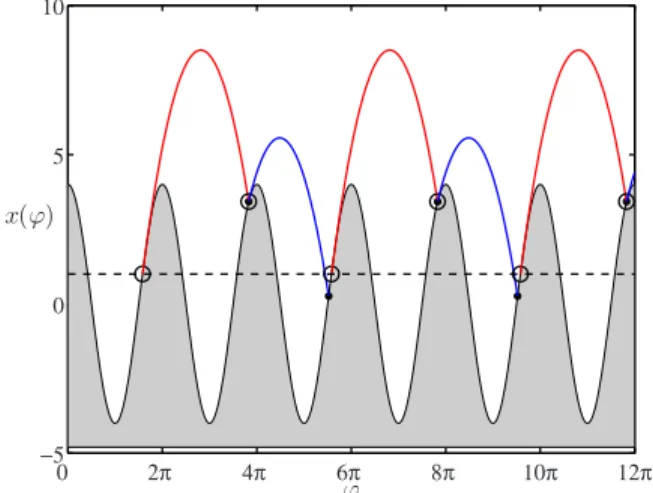
We choose every trajectory to begin at the first phase0for which ⌫ cos0= 1 and ⌫ sin0= −冑⌫2− 1⬍0. An example of trajectory is provided in Fig.1. The ball may impact in the zone where ⌫ cos⬎1 and bounce instantaneously. Other-wise, it sticks on the plate until it reaches⌫ cos= 1 where it takes off again, exactly as for the initial flight. Except in specific conditions that will be described below, the ball al-ways ends up impacting in the sticking region, which there-fore generates periodicity. By definition, a period-n motion involves n different flights 共e.g., period-2 in Fig. 1兲. The
sticking zone may be considered as a reset mechanism of the system: when the ball enters this zone, it forgets its past history.
The first flight time T satisfies⌫=⌫1共T兲, where ⌫1共T兲 ⬅
冑
1 +冢
T2 2 − 1 + cos T T − sin T冣
2 . 共4兲It is shown to be the highest possible flight time for a given ⌫ since the ball takes off with the maximum achievable ab-solute velocity
冑
⌫2− 1. The curve ⌫1共T兲 is monotonically increasing, which means that⌫1共T兲 is the smallest ⌫ required to observe T.
In general, T may be computed numerically by solving Eq.共2兲 for given 共⌫,0兲. This equation may be rewritten as a second-order polynomial equation in tan共0/2兲 which al-*[email protected]
Web site: http://www.grasp.ulg.ac .be
PHYSICAL REVIEW E 79, 055201共R兲 共2009兲
RAPID COMMUNICATIONS
ways have two solutions. Only one of them is in the ⌫ cos0ⱖ1 zone and is therefore physically relevant. In other words, there is always one and only one physical solu-tion0corresponding to a point in the共⌫,T兲 diagram which satisfies⌫ⱖ⌫1共T兲; this diagram contains all the information necessary to describe the motion.
For each different successive flight i, the computed flight time is reported on the 共⌫,T兲 diagram, where it forms a branch Bi as a function of ⌫ 共Fig. 2兲. As expected, all the
solutions are located below or on the curve⌫=⌫1共T兲, which mainly coincides with the branch B1except around T = 2N,
N苸N as explained later. The branch B2共⌬兲 decreases from
B1 to zero. More than two branches are observed around⌫ ⬃7.3. In the following, three kind of zones 共bouncing, stick-ing, and forbidden兲 are identified in the diagram, delimited by curves⌫BS共T兲, ⌫FB共T兲, and ⌫SF共T兲. A branch that switches
from a zone to another is related to a specific bifurcation of the system.
The bouncing zone corresponds to flights T that impact at a phase i=0+ T such as ⌫ cosiⱖ1, which is equivalent
to⌫ⱖ⌫BS共T兲, ⌫BS 2 =
冉
1 +T 2 2冊
2 − 2冉
1 +T 2 2冊
共T sin T + cos T兲 + T 2− 1 共sin T − T cos T兲2 . 共5兲 Since it may be shown that d⌫BS/dT has the same sign as共1−⌫ cos0兲, only the decreasing part of ⌫BSis relevant as a
separation between bouncing and sticking共Fig. 2兲. As seen
in Fig.3, a period-doubling bifurcation occurs when a branch crosses the ⌫BScurve from sticking to bouncing.
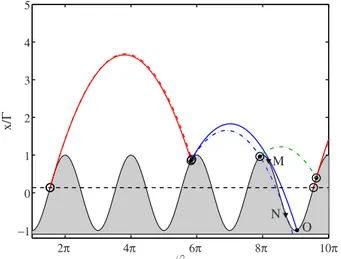
For some given accelerations, there is a range of flight times that cannot be experienced, as easily understood by inspecting Fig.4. The parabolic trajectory may be tangent to the forcing sinusoid, which means that the ball smoothly lands on the vibrated plate at tangent point M. Trajectories that lay above skip this landing opportunity and impact later 共after point O兲. On the other hand, trajectories that lay below impact and bounce before M and have a relatively short flight time T. This discontinuity in T is mainly due to the possibility for the free-flight parabola to intercept the forcing sinusoid in more than one point 共only the first intersection would correspond to a physically relevant impact兲. This to-pological transition is similar to the common tangent bifur-cation, which here results in incrementing or decrementing the number of flights by one. The flight time at point M is given by ⌫=⌫FB共T兲, where 0 2π 4π 6π 8π 10π 12π −5 0 5 10 ϕ x(ϕ)
FIG. 1. 共Color online兲 A plate is vibrated sinusoidally according to xp=⌫ cos 共shaded兲. The solid line is the trajectory x共兲 of a
completely inelastic ball let on this plate when⌫=4. The red 共re-spectively, blue兲 part corresponds to the first 共respectively, second兲 flight. The successive take-off phases 0 and impact phases 共0 + T兲 are represented by 共䊊兲 and 共쎲兲, respectively. The dashed hori-zontal line xp=⌫ cos=1 separates the bouncing and sticking zones. 0 2 4 6 8 10 0 π 2π 3π 4π 5π 6π Sticking Bouncing Forbidden Γ T
FIG. 2. 共Color online兲 共⌫,T兲 diagram. Shadings indicate the different zones 共bouncing, sticking, and forbidden兲, while colored symbol lines correspond to the branches Biof flight i obtained by
solving Eq.共2兲 numerically: 共䊊兲 B1,共䉭兲 B2,共쎲兲 B3, and next ones. The dashed curve corresponds to⌫1共T兲, the decreasing solid curve
corresponds to ⌫FB共T兲, the increasing solid curve corresponds to ⌫SF, and the decreasing solid curve corresponds to⌫BS. The dotted
lines indicate fixed points in T = 2N, with N苸N.
0 4π 8π 12π 16π 20π 24π −1 0 1 2 3 4 5 ϕ x/ Γ
FIG. 3. 共Color online兲 Period-doubling bifurcation. The solid trajectory 共⌫=7.320兲 sticks after three flights while the dash-dot trajectory共⌫=7.336兲 experiences five bounces before sticking at the sixth flight. Notations are the same as in Fig.1.
GILET, VANDEWALLE, AND DORBOLO PHYSICAL REVIEW E 79, 055201共R兲 共2009兲
RAPID COMMUNICATIONS
⌫FB=
T 2
冏
sin2T2
冏
. 共6兲
As for Eq. 共5兲, only the decreasing part of ⌫FB共T兲 is
physi-cally relevant 共Fig. 2兲. The other bound of the forbidden
region ⌫SF共T兲 is given by point O in Fig.4, for which the
position may be obtained numerically by solving Eq.共2兲 for
⌫=⌫FB. We note that there is another possibility for the
pa-rabola to be tangent to the sinusoid, i.e., at point N given by T/2=tan T/2, ∀⌫. Nevertheless, this second tangent point cannot be reached physically.
As mentioned previously, there are some trajectories that never enter the sticking region. Nevertheless, those trajecto-ries quickly converge to a periodic bouncing motion similar to the one encountered in the partially elastic ball 关1兴. A
period-1 motion is obtained for T = 2N and⌫ sin0= −N, ∀N苸N0. In the共⌫,T兲 diagram 共Fig.2兲, the numerical solu-tion leaves the curve ⌫1共T兲 and experiences a plateau in T = 2N. This fixed point of Eq. 共2兲 exists when ⌫
⬎
冑1 +
2N2. At each bounce, any perturbation from this equilibrium grows by a factor equal to the Floquet multiplierd共0+ T兲
d0
= 1 −
冑
⌫2−2N2. 共7兲 Therefore, the solution is stable when兩d共0+T兲d0 兩⬍1, i.e., until
⌫=
冑4 +
2N2. Period doubling occurs for larger values of⌫. The upper branch B1 quickly joins the ⌫1 curve, while the lower branch B2 enters the sticking zone at the same time.A deeper zoom in the range⌫苸关7.15,7.45兴 of the 共⌫,T兲 diagram reveals an intricate structure 共Fig.5兲 generated by
the successive bifurcations occurring each time a branch changes of zone. Branches of odd-degree共respectively, even兲 monotonically increase 共decrease兲 with an increase in ⌫. When a branch crosses one of the horizontal lines T = 2N,
every branch of higher degree should cross the line at the same accumulation point ⌫S. This is easily understood by
inspecting Fig. 6, which corresponds to acceleration very close to⌫S⯝7.253 378: at first bounce, the ball lands in the
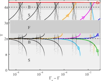
vicinity of the unstable fixed point T = 2N. If landing is located exactly on this point, every further impact should occur at the same phase, which explains the branch crossing. But any small disturbance is amplified and the trajectory eventually reaches the sticking zone after a finite but arbi-trarily large number of bounces. An infinity of branches has to be created through an infinity of bifurcations converging to the accumulation point. A second infinity of bifurcations annihilates those branches at⌫ⲏ⌫S. A logarithmic zoom on
⌫S reveals that this cascade of bifurcations is self-similar
共Fig. 7兲. A complex branch pattern is repeated indefinitely
with a scaling factor of 30.67, different from the Feigenbaum constant. Inside this pattern, branches are seen to regularly
2π 4π 6π 8π 10π −1 0 1 2 3 4 5 M N O ϕ x/ Γ
FIG. 4. 共Color online兲 Saddle-node bifurcation. The trajectory may be tangent to the forcing sinusoid in points M and N. The solid trajectory共⌫=7.15兲 just passes point M, impacts in O and sticks after two flights while the dash-dot trajectory 共⌫=7.20兲 impacts before M and so experiences three flights before sticking. Notations are the same as in Fig.1.
7.15 7.2 7.25 7.3 7.35 7.4 7.45 0 π 2π 3π 4π S B F S B Γ T
FIG. 5. 共Color online兲 Zoom in the range ⌫苸关7.15,7.45兴 of the 共⌫,T兲 diagram. 共䊊兲 B1,共䉭兲 B2,共䊐兲 B3,共䉮兲 B4,共〫兲 B5,共⊲兲 B6, and
共·兲 Bi, with i⬎6. The dashed lines correspond to T=2N. The
bullet 共쎲兲 denotes the accumulation point ⌫S⯝7.253 378, where
branches Bi, iⱖ2 intersect each others in T=2. Other notations are the same as in Fig.2.
0 6π 12π 18π 24π 30π 36π −1 0 1 2 3 4 5 ϕ x/ Γ
FIG. 6. 共Color online兲 Typical trajectory that occurs when branches Bi, iⱖ2 enter into the vicinity of the unstable fixed point
T = 2. Notations are the same as in Fig.1.
COMPLETELY INELASTIC BALL PHYSICAL REVIEW E 79, 055201共R兲 共2009兲
RAPID COMMUNICATIONS
cross the T = 4 line, giving birth to infinity of other accu-mulation points and related bifurcation cascades. And finally, some nonconsecutive branches m and n may also intersect in other locations than T = 2N, which correspond to the un-stable repetition of sequences made of 兩m−n兩 different flights; a cascade of bifurcations is also related to each of
those intersections. The resulting branch structure observed in the range ⌫苸关7.18,7.44兴 共Fig. 5兲 is thus an infinitely
complex object; denumerability of the occurring bifurcations is still an open question. However, trajectories never become chaotic and, stricto sensu, the Lyapunov exponent is negative on each periodic solution: sufficiently small perturbations, either on the initial condition0or on the forcing parameter ⌫, quickly vanish and do not qualitatively modify the trajec-tory. Conversely, a highly sensitive dependence on initial conditions and parameters is observed when finite perturba-tions are considered.
In conclusion, this Rapid Communication presents an ana-lytical solution of the inelastic ball bouncing on a vibrated plate. Different zones are identified on the 共⌫,T兲 diagram, transitions between them are related to tangent and period-doubling bifurcations. An infinity of bifurcation cascades is observed in a finite range ⌫苸关7.18,7.44兴, leading to an in-tricate structure of the bifurcation diagram, although trajec-tories never become strictly chaotic.
T.G. and S.D. thank FRIA/FNRS for financial support. We gratefully acknowledge M. Guilmet, R. Sepulchre, and H. Croisier for fruitful discussions. This project was a part of IAP-P6/17 fro the Belgian Science Policy and COST-P21 actions.
关1兴 N. B. Tufillaro, T. Abbott, and J. P. Reilly, An Experimental Approach to Nonlinear Dynamics and Chaos 共Addison-Wesley, Reading, MA, 1992兲.
关2兴 R. B. Davis and L. N. Virgin, Int. J. Non-linear Mech. 42, 744 共2007兲.
关3兴 S. Dorbolo, D. Volfson, L. Tsimring, and A. Kudrolli, Phys. Rev. Lett. 95, 044101共2005兲.
关4兴 A. Kudrolli, G. Lumay, D. Volfson, and L. S. Tsimring, Phys. Rev. Lett. 100, 058001共2008兲.
关5兴 T. Gilet and J. W. M. Bush, Phys. Rev. Lett. 102, 014501 共2009兲.
关6兴 G. A. Luna-Acosta, Phys. Rev. A 42, 7155 共1990兲.
关7兴 S. N. Majumdar and M. J. Kearney, Phys. Rev. E 76, 031130 共2007兲.
关8兴 E. D. Leonel and M. R. Silva, J. Phys. A: Math. Theor. 41, 015104共2008兲.
关9兴 Y. Fang, M. Gao, J. J. Wylie, and Q. Zhang, Phys. Rev. E 77, 041302共2008兲.
关10兴 V. Milner, J. L. Hanssen, W. C. Campbell, and M. G. Raizen,
Phys. Rev. Lett. 86, 1514共2001兲. 关11兴 E. Fermi, Phys. Rev. 75, 1169 共1949兲.
关12兴 Y. Chen, M. Bibole, R. Le Hazif, and G. Martin, Phys. Rev. B 48, 14共1993兲.
关13兴 S. Ramachandran and G. Lesieutre, J. Vibr. Acoust. 130, 021008共2008兲.
关14兴 H. Katsumata, V. Zatsiorsky, and D. Sternad, Exp. Brain Res. 149, 17共2003兲.
关15兴 R. Ronsse, P. Lefèvre, and R. Sepulchre, Neural Networks 21, 577共2008兲.
关16兴 F. Melo, P. B. Umbanhowar, and H. L. Swinney, Phys. Rev. Lett. 75, 3838共1995兲.
关17兴 I. S. Aranson and L. S. Tsimring, Rev. Mod. Phys. 78, 641 共2006兲.
关18兴 J. M. Pastor, D. Maza, I. Zuriguel, A. Garcimartín, and J.-F. Boudet, Physica D 232, 128共2007兲.
关19兴 A. Mehta and J. M. Luck, Phys. Rev. Lett. 65, 393 共1990兲. 关20兴 J. M. Luck and A. Mehta, Phys. Rev. E 48, 3988 共1993兲.
10−8 10−6 10−4 10−2 0 π 2π 3π 4π S B F S B Γs− Γ T
FIG. 7. 共Color online兲 Zoom in the self-similar cascade of bi-furcations converging to the accumulation point ⌫S⯝7.253 378.
Notations are the same as in Fig.5.
GILET, VANDEWALLE, AND DORBOLO PHYSICAL REVIEW E 79, 055201共R兲 共2009兲
RAPID COMMUNICATIONS