Experimental Study of Sub-aerial, Submerged and Transitional Granular Slides in Two and Three Dimensions

POLYTECHNIQUE MONTRÉAL

Experimental Study of Sub-aerial, Submerged and Transitional Granular

Slides in Two and Three Dimensions

MOHAMAD PILVAR

Département des Génies civil, géologique et des mines

Mémoire Présenté en vue de l’obtention du diplôme de Maîtrise ès sciences appliquées Génie Civil

Août 2019

POLYTECHNIQUE MONTRÉAL

Ce mémoire intitulé:

Experimental Study of Sub-aerial, Submerged and Transitional Granular

Slides in Two and Three Dimensions

Présenté par Mohamad PILVAR

en vue de l’obtention du diplôme de Maîtrise ès sciences appliquées a été dûment accepté par le jury d’examen constitué de :

Elmira HASSANZADEH, présidente

Ahmad SHAKIBAEINIA, membre et directeur de recherche Musandji FUAMBA, membre

DEDICATION

À tous ceux qui restent toujours curieux et qui prennent le temps d’y penser. Adaptée de Bruce Benamran

ACKNOWLEDGEMENTS

The work presented in this thesis would not have been possible without the support of many dedicated people. I am particularly indebted to my master’s supervisor Dr. Ahamd Shakibaeinia, for his mentorship, patience, and support throughout all stages of this study. He is one of the distinguished humans I ever got to know.

I would also like to thank the members of my thesis committee for their effort and time in reviewing my thesis with their valuable comments and suggestions. I would like to thank Javad Pouraghniaei in providing experimental data for my thesis.

I would also acknowledge the financial support of the Natural Sciences and Engineering Research Council of Canada (NSERC) and Polytechnique Montreal. I would like to also thank Mr. Étienne Bélanger for his assistance in setting up the experiments.

Finally, I would like to thank my parents, siblings, and friends for their great support and encouragement. Thank you all for always being there for me.

RÉSUMÉ

Les glissements de terrain sont reconnus comme des dangers naturels avec des dommages majeurs qui peuvent causer un danger pour la vie humaine et/ou des pertes matérielles en raison de leur comportement destructeur. Ils se produisent généralement près des régions montagneuses (classées comme des glissements de terrain non submergés ou sous-aériens) ou près des zones côtières telles que les océans, les lacs, les berges des rivières, les baies (considérées comme des glissements de terrain sous-marins) qui génèrent des vagues destructrices de grande amplitude, semblables à des tsunamis.

Les glissements de terrain déformables peuvent généralement être considérés comme le mouvement descendant d'un matériau granulaire sur un plan incliné et / ou sur un terrain plat en raison de leur comportement. À cet égard, dans cette étude, la glissière de matériaux granulaires générée par la gravité pour différents angles de pente, types de matériaux, rugosité de lit et régimes d'écoulement dans des configurations expérimentales en 2D et 3D a été étudiée expérimentalement. L’objectif de cette recherche est d’identifier les effets des facteurs sur la morpho-dynamique (formes de dépôt et longueur de déplacement) et la structure d’écoulement interne des matériaux granulaires lors du glissement sur un plan incliné. En outre, cette étude fournit des données de qualité pour le paramétrage et la validation des modèles numériques.

En ce qui concerne la méthode expérimentale utilisée dans cette étude, la diapositive des deux types de matériaux granulaires (billes de verre et sable) est considérée sur les surfaces inclinées rugueuses et lisses avec des angles de pente différents selon trois régimes d'écoulement différents, sous-aérien (sec) , submergé (sous l’eau) et transitoire (matières sèches envahissant le plan d’eau). Les expériences sont menées au laboratoire hydraulique de Polytechnique de Montréal dans un réservoir rectangulaire en plexiglas. Un plan incliné et une porte coulissante sont placés dans le réservoir afin de créer un amoncellement de la masse granulaire initialement en forme triangulaire au sommet du plan incliné, maintenu par la porte. La libération des matériaux granulaires est déclenchée en soulevant la porte. L'évolution de l'écoulement de la masse granulaire est ensuite capturée et visualisée lors du retrait de la porte à l'aide d'une caméra à haute vitesse. Une méthode optique bien testée, appelée technique PIV (Particle Image Velocimetry), est utilisée pour extraire les champs de vecteurs vitesse.

En comparant l'évolution temporelle de ces trois régimes, les matériaux granulaires sous-aériens ont été observés de glisser par la pente en montrant une distribution bien uniforme des matériaux avec une vitesse supérieure (2 à 3 fois) à celle du cas immergé. Cependant, un front d'écoulement plus épais avec une forme parabolique et une circulation forte ont été observés pour le cas immergé. Le comportement des cas en transition s’est révélé être similaire à celui des cas sous-aériens et submergés, respectivement avant et après l’entrée de la masse granulaire dans l’eau. Le moment de l'entrée présentait un comportement plus complexe à cause de la cohésion supplémentaire due à la saturation partielle et à l'impact de la vague.

Le régime de glissement se révèle être le facteur principal affectant la morpho-dynamique granulaire. La variation de la distance de parcours en fonction du temps pour les cas sous-aériens et submergés présente des tendances similaires pour trois parties (accélération, écoulement constant et décélération) mais avec des échelles spatio-temporelles différentes. Les tendances transitoires montrent toutefois une décélération et une réaccélération supplémentaires. Les observations suggèrent que l’influence de l’angle de glissement, du type de matériau et de la rugosité du lit est moins grande en présence d’eau.

Une solution analytique basée sur la rhéologie de µ (I) utilisant un écoulement non permanent comme hypothèse est utilisée et s'est avérée utile pour la prédiction du mouvement de la masse granulaire. Ce modèle est capable de reproduire le profil de vitesse logarithmique du cas sous-aérien avec une précision acceptable. Pour les cas d'immersion, bien que les effets de la force de traînée et de la poussée d’Archimède (force de levage) aient été pris en compte dans ce modèle, celui-ci était moins précis et surestimait les valeurs de la vitesse CDM lorsque les résultats du modèle étaient comparés aux résultats expérimentaux. Par conséquent, comme recommandations générales, pour les travaux futurs, l’effet de circulation et de turbulence (et l’effet lubrifiant) pourraient être introduits et mis en œuvre dans ce modèle théorique afin d’obtenir une meilleure compatibilité et un meilleur accord avec les résultats expérimentaux.

ABSTRACT

Landslides are recognized as natural hazards with massive casualties and loss of properties due to their damaging behavior. They usually happen near the mountainous regions (classified as unsubmerged or sub-aerial landslides) or near coastal areas such as oceans, lakes, riverbanks, bays (considered as submarine landslides) that generates destructive tsunami-like waves with high amplitudes.

Deformable landslides usually can be regarded as the downward movement of granular material on an inclined and/or flat plane due to their nature. In this regard, in the present study, we experimentally investigate the gravity-driven slide of granular materials for various slope angles, material types, bed roughness, and flow regimes in 2D and 3D experimental setups.

The objective of this research is to identify the effects of so-called factors on the morpho-dynamics (deposit shapes and run-out length) and the internal flow structure of the granular materials during the slide over an inclined plane. Also, the present study provides quality data for parameterization and validation of the numerical models.

Regarding the experimental method used in the present study, the slide of two types of granular materials (glass beads and sand) is considered on the rough and smooth inclined surfaces with different slope angles in three different flow regimes, namely sub-aerial (dry), submerged (underwater) and transitional (dry materials intruding the water body) regimes. Experiments are carried at the hydraulic laboratory of Polytechnique Montreal in a rectangular Plexiglas tank. An inclined plane and a sliding gate are placed within the experimental tank to create a wedge-shape initial pile of the granular mass at the top of the inclined plane, hold by the gate. The release of granular materials is triggered by lifting the gate. The flow evolution of the granular mass is then captured and visualized upon the removal of the gate using a high-speed camera. A well-tested optical method called Particle Image Velocimetry (PIV) technique is applied to extract the velocity vector fields.

By comparing the time history evolution of these three regimes, one can recognize that the sub-aerial slides moved down the slope by showing a well-uniformed distribution of the materials with a higher speed (2-3 times) than the submerged counterpart case. However, a thicker flow front with parabolic-like shape and strong circulation were observed for the submerged case. The behavior of

transitional cases was found to be similar to the sub-aerial and submerged cases, before and after the granular mass enters the water, respectively. The moment of entry, however, presented a more complex behavior as the result of additional cohesion, partial saturation, and the wave impact. The slide regime is found to be a major controller of the granular morpho-dynamic. The time history of the runout distance for the sub-aerial and submerged cases present similar three-parts (acceleration, steady flow, and deceleration) trends tough with different spatiotemporal scales. The transitional trends, however, show additional deceleration and reacceleration phases. The observations suggest that the impact of slide angle, material type, and bed roughness is less significant in the presence of water.

An analytical solution based on the µ (I) rheology with the unsteady assumption is utilized and shown to be useful in the prediction of the motion of the granular mass. This model is able to produce the logarithmic velocity profile of the sub-aerial case with acceptable accuracy. For submerge case, although the effects of drag as well as buoyancy forces (lifting force) of ambient fluid were taken into account in this model, it was less accurate by overestimating the values of COM velocity when it was tested against experimental results. Therefore, as general recommendations, for the future works, the circulation, the turbulence effects, and lubrication effect could be introduced and implemented into this theoretical model for producing better compatibility and agreement with experimental results.

TABLE OF CONTENTS

INTRODUCTION ... 1

LITERATURE REVIEW ... 2

PROCESS AND ORGANIZATION OF THE WORK ... 12

ARTICLE 1: TWO-DIMENSIONAL SUB-AERIAL, TRANSITIONAL, AND SUBMERGED GRANULAR SLIDES ... 14

4.1 Introduction ... 15

4.2 Experimental setup and procedures ... 17

4.2.1 Experimental setup and materials ... 17

4.2.2 Experimental procedures and data acquisition ... 18

4.2.3 Image processing ... 19

4.3 Results and discussions ... 21

4.3.1 Sliding phenomenology and morphology ... 21

4.3.2 Internal flow structure ... 29

4.4 Theoretical models ... 34

4.4.2 Submerged case ... 37

4.4.3 Comparison with experiments ... 39

4.5 Conclusion ... 40

THREE-DIMENSIONAL SUB-AERIAL, TRANSITIONAL, AND SUBMERGED GRANULAR SLIDES ... 42

5.1 Experimental setup and procedures ... 42

5.1.1 Experimental setup and materials ... 42

5.1.2 Experimental Procedures and data acquisition tool ... 45

5.1.3 The image processing technique – Particle Image Velocimetry (PIV) ... 46

5.2 Results and discussions ... 48

5.2.1 The morphodynamics of the granular sliding ... 48

5.2.2 Internal flow structure ... 52

GENERAL DISCUSSION ... 74

CONCLUSION AND RECOMMENDATIONS ... 76

REFERENCES ... 78

LIST OF TABLES

Table 2.1 Ten major landslides in Canadian History ... 4

Table 4.1 Summary of experimental conditions ... 20

Table 4.2 Rheological parameters of the theoretical model ... 40

Table 5.1 Summary of experimental conditions ... 46

LIST OF FIGURES

Figure 2.1 Schematic view of a sub-aerial landslide, L denotes the run-out distance [11] ... 2 Figure 2.2 The Frank slide in 1996 [39] ... 3 Figure 2.3 The complete outline of the Mount Meager landslide showing the initiation zone (A– B), the two major bends (C and E), the facing wall of Meager Creek (F), and the bifurcated flow that traveled up Meager Creek, and across the Lillooet River (G). [35] ... 3 Figure 2.4 Schematics view of experimental configurations performed by Lajeunesse et al.[43] (a)

the rectangular channel and (b) the “semiaxisymmetric” setup ... 6 Figure 2.5 Scaled distance traveled by the pile foot [Lt-Li/Li] as a function of t/τc. (a) a=0.6, M

=470 g, Li=102 mm. (b) a=2.4, M =560 g, Li=56 mm. (c) a=16.7, M =170 g, Li=10 mm. [43] ... 7 Figure 2.6 Normalized granular spreading length versus normalized time from experimental and

numerical tests [16] ... 8 Figure 2.7 Evolution of run-out length as a function of normalized time (a) loose (b) dense regimes

[19] ... 10 Figure 4.1 (a) Schematic and (b) photograph of the experimental ... 18 Figure 4.2 Snapshots of slide of glass-beads material on a 45° smooth surface. (a) Sub-aerial slide

(case D7) , (b) Submerged slide (case S7) and (c) Transitional slide (case T7) ... 24 Figure 4.3 Time sequences of slide of glass-beads material on a 45° smooth surface. (a) Sub-aerial

slide (Case D3), (b) Submerged slide and (c) Transitional slide ... 26 Figure 4.4 Comparison of the normalized runout length for 45° granular sliding with (a) glass

beads and smooth surface, (b) glass beads and rough surface, (c) sand and smooth surface, (d) sand and rough surface, and 30° sliding with (e) glass beads and smooth surface, (f) glass beads and rough surface, (g) sand and smooth surface, (h) sand and rough surface. ... 28 Figure 4.5 Comparison of the normalized runout length of dry (sub-aerial) granular sliding of (a)

Figure 4.6 G-PIV velocity vectors field for a sub-aerial slide (case D5). ... 30

Figure 4.7 Experimental and theoretical (a) velocity profile at T=3 and (b) time history of the center of mass velocity for the sub-aerial case D5. ... 31

Figure 4.8 G-PIV velocity vectors field for a submerged slide (case S7) ... 32

Figure 4.9 Experimental and theoretical (a) velocity profile at T=3 and (b) time history of the center of mass velocity for the submerged case S7. ... 33

Figure 4.10 G-PIV velocity vectors (left) and velocity magnitude field (right) for a transitional slide (case T7) at the moment of impact (T=2). The dashed and dotted lines show approximate water and granular surfaces, respectively. ... 34

Figure 4.11 Velocity profile of monodirectional motion of granular flows down an inclined plane ... 35

Figure 4.12 Theoretical velocity profiles for cases D5 (solid line) and S5 (dashed line) ... 40

Figure 5.1 Schematic sketch of the 3D experimental setup ... 44

Figure 5.2 The sketch of granular sliding, plan view ... 45

Figure 5.3 Snapshots of slide of glass-beads material on a 45° smooth surface, sub-aerial regime ... 55

Figure 5.4 Snapshots of slide of glass-beads material on a 45° smooth surface, submerged regime ... 56

Figure 5.5 Snapshots of slide of glass-beads material on a 45° smooth surface, transitional regime ... 57

Figure 5.6 Comparison of the normalized runout length of 45° granular sliding with (a) Glass beads and smooth surface (b) Glass beads and Rough surface (c) Sand and Smooth surface(d) Sand and Rough surface, and 30° sliding with (e) Glass beads and Smooth surface and (f) Sand and Smooth Surface ... 58

Figure 5.7 Comparison of the normalized runout length of dry (sub-aerial) granular sliding of (a) 45° slope angle, and (b) on 30° slope angle ... 59

Figure 5.8 Snapshots of slide of glass-beads material on a 45° smooth surface, sub-aerial slide (top view) ... 60 Figure 5.9 The final deposit shape of sliding of glass-beads material on the 45° smooth surface at

T=6 (final stage) ... 61

Figure 5.10 Time sequences of slide of glass-beads material on a 45° smooth surface from the top view, (a) Sub-aerial slide, (b) Transitional slide and (c) Submerged slide ... 62 Figure 5.11 Time sequences of slide of sand material on a 45° smooth surface from the top view,

sub-aerial slide ... 64 Figure 5.12 Comparison of the normalized lateral runout length of glass beads sliding on the

smoothed 45° surface for different flow regimes ... 64 Figure 5.13 G-PIV velocity vectors (left column) and velocity magnitude field (right column) of

glass-beads material slide on a 45° smooth surface in (a) the sub-aerial, (b) transitional and (c) submerged cases ... 65 Figure 5.14 Velocity profiles of sliding of glass-beads material on a smoothed 45° in (a) sub-aerial

regime at T=1.5 and (b) submerged regime at T=4 ... 67 Figure 5.15 G-PIV velocity vectors (left column) and velocity magnitude field (right column) of

the sand material slide on a 45° smooth surface in (a) the sub-aerial, and (b and c) submerged cases ... 68 Figure 5.16 G-PIV velocity vectors (left column) and velocity magnitude field (right column) of

the submerged slide of glass-beads material on a 45° rough surface at T=5.0 ... 69 Figure 5.17 G -PIV velocity vectors (left column) and velocity magnitude field (right column) of

the glass-beads material slide on a 30° smooth surface in (a) the sub-aerial, (b) submerged cases ... 70 Figure 5.18 G -PIV velocity vectors (left column) and velocity magnitude field (right column) of

the sand material slide on a 30° smooth surface in (a) the sub-aerial, (b) submerged cases . 71 Figure 5.19 G -PIV velocity vectors (left column) and velocity magnitude field (right column) of

LIST OF SYMBOLS AND ABBREVIATIONS

COM Center of Mass

DEM Discrete Element Method

MPS Moving Particle Semi-Implicit Method PIV Particle Image Velocimetry

SPH Smoothed-Particle Hydrodynamics

µ(I) Friction Coefficient

I Inertia number

pm Mechanical pressure σ Cauchy stress tensor

p Pressure

τ Deviatoric part of the stress tensor I Unit tensor

ρb Bulk density

ρf Fluid density

ρg Grain density

θs Static frictional angles

θ2 Dynamic frictional angles

I0 Empirical coefficient constant

μs Static friction coefficient

μ2 Dynamic friction coefficient

θr Angle of repose

u Particle velocity vector

INTRODUCTION

Gravity-driven flows of granular media down a slope is ubiquitous in many industrial, natural, and engineering contexts. In nature, for example, granular slides are commonly recognized as the natural hazards, with notable examples being landslides, debris flows, and rock avalanches. Two destructive impacts can be associated with the granular slides: (a) direct, which occurs through the overland flow of granular mass and (b) indirect impacts by generating tsunami waves within the nearby area, infrastructures, and human properties. Therefore, identifying their physical mechanisms and characteristics (e.g., morphodynamic runout length and kinetic energy) plays a critical role in the mitigation of their damaging impacts and hazard management [1-7].

The dynamics of granular slides can be affected by various conditions, such as slope angle, material type, and flow regime. Particularly, based on the presence of surrounding fluids, landslides can be recognized as three groups: The first type is known as the sub-aerial or dry slide [1, 2, 6-16], where the interstitial fluid is composed of a gas (e.g., air) and a free-fall granular flow regime is dominant. Such landslides occur in non-aquatic environments such as the mountainous area. The second group is classified as the submerged slides [3, 8, 17-27], where the ambient fluid is a liquid (e.g., water), creating a multiphase grain-inertial (and sometimes micro-viscous) granular flow regime. Sub-aquatic landslides belong to this group. The third group is a transitional slide [26, 28, 29], which is a transition between the two previous groups. The granular media becomes submerged as it enters the water. In addition to the surge wave impact, the simultaneous presence of gaseous and liquid phases in the ambient and interstitial fluids near the entry point (a partially-saturated region) creates more complexity of predictions. Such slides are common features of the coastal/fluvial slope failures and landslides.

In this work, we experimentally investigate the granular slides in two and three dimensions in Chapter 4 and Chapter 4, respectively. The specific objectives of this thesis are (a) to shed light into the complex physics (morpho-dynamics and flow structure) of these granular flows, (b) also to provide comprehensive benchmarks for validation and parametrization of the numerical models (c) to develop an unsteady rheological model based on the µ (I) friction law to describe the rheology of granular materials and (d) to analyze the internal flow structure by using a multi-grid multi-step MATLAB code called PIVlab developed by Thielicke and Stamhuis [30, 31].

LITERATURE REVIEW

The dynamics of landslides can be identified as the slope failure or rapid movement of granular materials flowing down an inclined plane and spreading on a horizontal plane as depicted in Figure 2.1. Landslides in nature can cause loss of lives and property damages. In Canadian history, Frank Slide is known as one of the deadliest landslides occurred on April 29, 1903, due to the rock avalanches down Turtle Mountain. About 110 people were killed because of this rock slide [32]. Pandemonium Creek Slide (1959) [33] and Saint-Jean-Vianney landslides (1971) [34] with huge destructive impacts are other examples of landslides in past decades.

Figure 2.1 Schematic view of a sub-aerial landslide, L denotes the run-out distance [11] Landslides can cause even more fatalities when they occur underwater and produce tsunami-like waves near the shorelines and river banks. For instance, in the case of Meager landslide [35], the debris flow created two landslide dams, one on Meager Creek and the second one on Lillooet River with a maximum speed of 60 m/s [36]. Another example is Lituya Bay landslide, Alaska (1958), which was triggered by a rock slide into a fjord in Alaska. The latter one generated a surge wave of 534 m with a mean velocity of 110 m/s at the impact zone [37, 38].

According to a publication from Natural Resources Canada, Geological Survey of Canada, ten major and destructive landslides can be identified in Canadian history sorted in chronological order as shown in Table 2.1.

Figure 2.2 The Frank slide in 1996 [39]

Figure 2.3 The complete outline of the Mount Meager landslide showing the initiation zone (A– B), the two major bends (C and E), the facing wall of Meager Creek (F), and the bifurcated flow

Table 2.1 Ten major landslides in Canadian History

No. Year of occurrence Place of occurrence Description of the landslide

1 1971 St-Jean-Vianney, QUE Liquefied clay due to the heavy

rain

2 1957 Taylor, B.C Landslide of Cretaceous rocks

3 1929 Burin Peninsula (Grand Banks landslide), NFLD

Underwater landslide led to a deadly tsunami

4 1921 Britannia Beach, B.C Release of a roaring torrent into

the creek

5 1915 Jane Camp, B.C A large landslide of rock, mud,

and snow

6 1909 Burnaby, B.C Derailed a work train

7 1908 Notre-Dame-de-la-Salette, QUE A landslide of Leda clay

8 1903 Frank, AB Rock avalanche from Turtle

Mountain

9 1891 North Pacific Cannery, B.C Heavy rains ruptured a dam

created by a previous landslide

10 1889 Quebec City, QUE An overhanging piece of rock

Since 1840, landslides in Canada have led to over 600 fatalities and have cost Canadians billions of dollars – with annual costs reaching approximately $200 - 400 million. Therefore, it is critical to understand their flow morphodynamics which enables us to predict their run-out length in two directions (longitudinal and lateral travel distances), estimate their velocity vector fields and reduce their catastrophic impacts.

Past studies on landslides have included the laboratory experiments as well as numerical simulations (e.g. [2, 6, 8-11, 13, 17-22, 28, 29, 37, 40-42] ) with various conditions. To name but a few, slope inclination angle, material type, and flow regimes can control the morphodynamics

and morphology of landslides. Particularly, for material type, one can categorize past experiments into rigid [40, 41] or/ deformable granular media (e.g. [37]). Another notable classification is based on the ambient fluid. When landslides occur in the non-aquatic environment (under air), they are called sub-aerial landslides. In this regard, many attempts, including experimental-scale work, have been done to investigate the dynamics of sub-aerial landslides. For example, the collapse of the granular column over a flat plane was studied by Lajeunesse et al. [43]. Two different setup configurations were used in their experimental works, as shown in Figure 2.4. They explored the effect of geometry on flow dynamics and morphology. The material they used for the slumping was glass beads of the mean diameter of either d =1.15 mm or d=3 mm. For both geometries, it was found that the internal flow structure was mainly dependent on the initial aspect ratio (a=Hi/Li) of the granular column where Hi denotes the height of the initial granular column and Li represents its length along the flow direction. For presenting their results, the characteristic time scale of

τc=Hi/g was used as the time it takes for the free fall of the granular column. The results for the normalized horizontal travel distance of pile frontier (L-Li/Li ) was displayed versus the characteristic time scale of t/τc for three different values of a. It was reported that the initial aspect ratio does not affect the time scale of flow evolution.

A closer inspection of Figure 2.5 and Figure 2.6 shows that the evolution of the granular column has three distinguished phases, namely (a) acceleration phase (lasting approximately 0.8τc ) upon the release of material, which is followed by a relatively long time scale of the (b) steady-state phase which lasts 1.9τc. Finally, the flow slows down at the (c) declaration phase and comes to rest after the elapsing time scale of 0.6τc. Similar trend and behaviors have been reported by other studies dealing with collapses of granular columns.

To name but a few, [16, 38, 44, 45] showed an S-shape curve for sub-aerial granular slides and slumps. Also, a common feature during the granular material collapse over a horizontal plane was reported by these studies. The granular assembly stretches and becomes thinner at the front, as the grains of flowing layer (above the static layer) fail. This might suggest that total run-out length of flow front might be significantly longer than the spreading of the center of mass of granular assembly [11].

Figure 2.4 Schematics view of experimental configurations performed by Lajeunesse et al.[43] (a) the rectangular channel and (b) the “semiaxisymmetric” setup

Figure 2.5 Scaled distance traveled by the pile foot [Lt-Li/Li] as a function of t/τc. (a) a=0.6,

Figure 2.6 Normalized granular spreading length versus normalized time from experimental and numerical tests [16]

Experimental studies on the spreading of dry granular materials over a rough inclined plane were the subject of many past studies (e.g., [7, 13, 46, 47]). For example, Pouliquen and Forterre [7] developed depth-averaged mass and momentum conservation equations for granular flows originally derived by Savage and Hutter [5]. Then a friction law was introduced into their hydrodynamic model to incorporate the effect of bed roughness. The predictions obtained by this model was tested against their experimental results.

Y. Zhou et al. [2] investigated the morphology and final deposit shape of dry landslide dam with grains of non-uniform sizes. The factors they considered for the sliding were sliding area length, angle of inclination, and the bed roughness. They showed that the larger slope angle produced a wider final deposition shape of granular materials with a higher crust surface frontal angle. Also, it was found that by increasing the sliding area and bed friction coefficient, more separation in grain sizes will occur. The same behavior was observed when the slope angle was increased. However, by decreasing the slope angle, the main direction of normal contact force switched to other directions. Their numerical approach was PFC 3D software to explore the influence of some topographies features on the final deposit shape and morphology of landslide dams.

Utili et al. (2015) (T1)

Regarding numerical simulations, many attempts have been made to shed light into the complex physics of granular flows in sub-aerial, transitional ( intruding into the water) and submarine landslides. By determining their flow dynamics, one can predict their run-out length in two directions (longitudinal and lateral travel distances), estimate their velocity vector fields and therefore reduce the risk associated with their damaging impacts. Among these numerical approaches, Ashtiani et al. [3] studied the deformation of landslides as well as the amplitude of tsunami waves generated by the landslides for three initial submergence conditions for the sliding mass namely subaerial (SAL) semisubmerged (SSL), and a submarine (SML) landslide. They applied a second-order finite volume numerical model called 2LCMFlow model to investigate the so-called interactions between landslide and water by considering landslide as a two-phase Coulomb mixture. In another study [2], they used the Discrete Element Method (DEM) model to simulate the dry landslide. They employed PFC 3D software to explore the influence of some topographies features on the final deposit shape and the morphology of landslide dams.

Landslide problems have also been conducted by Kheirkhahan et al. [24] to study the granular column collapse as well as dry and submerged landslides through an open-source code called SPHysics2D (a mesh-free Lagrangian method). It is worth mentioning that in their two-phase model, µ (I) viscoplastic model is utilized for the solid phase (glass beads). Another numerical scheme to model the dry granular materials intruding a water body was introduced in [26] on the open-source platform, OpenFOAM®, which uses the finite volume method (FVM) method for discretization. The validation of their numerical simulations has been done by comparing their results with experiments done by Viroulet et al. [29]. Another numerical study on the morphodynamics of dry and submerged (saturated) granular sliding was carried out by Kumar et al. [19] to explore the role of initial volume fraction on the evolution of granular column slump in the fluid. In this work, various slope angles were used to conduct the numerical simulations, namely 0°, 2.5°, 5°, and 7.5°. The results obtained by their numerical simulations, as shown in Figure 2.7 reveals that for dense granular media, dry cases showed relatively higher values of run-out length evolution compared to similar submerged cases. The drag force that was experienced by grains in saturated regimes can explain this difference between dry and saturated regimes evolution. This induced drag force acts as a resistant to the movement of granular materials resulting in less

run-out length for submerged cases. The opposite behavior is observed for loose media as the granular materials experience less drag force in comparison with the dense initial packing condition.

Figure 2.7 Evolution of run-out length as a function of normalized time (a) loose (b) dense regimes [19]

(a)

There are some other studies which give us better understating of the dynamics of landslides over complex geometry [1], or another investigation has been proposed in [25] for the collapse of immersed granular columns as an ideal indication of a submarine landslide by using an Eulerian-Eulerian two-phase model based on a collisional-frictional law for the granular. Parez el al. [10, 11, 18] explored the granular mass flowing down a slope when the flow is in its unsteady state. 2D DEM simulation results have been compared with the analytical solutions to come up with the velocity profiles and also stress fields for acceleration and deceleration phases of the flow. Tajnesaei et al. [38] used the weakly compressible moving particle semi-implicit method called MPS (mesh-free based particle methods) to model both rigid and deformable-body of a flowing mass into a water body, sub-aerial and submerged landslides. Then the results of final deposit shapes were compared and validated against the available experimental measurements and past numerical results such as [20, 48, 49].

Although the widespread experimental works and numerical simulations have been carried out on landslides in two-dimensions, there is a lack of comprehensive study on the experimental laboratory-scale works as robust standards to validate the aforementioned numerical results. Therefore, the present study will address this issue by experimentally study the sub-aerial, transitional, and submerged granular slides in two dimensions (Chapter 4) and three dimensions (Chapter 5), for various slope angles, material types, and bed roughness. The goal is to shed insight into the complex morpho-dynamics and flow structures of these granular flows, also to provide comprehensive benchmarks for validation and parametrization of the numerical models.

PROCESS AND ORGANIZATION OF THE WORK

As discussed in Chapter 2, even though numerous experimental studies and computer simulations exist on the slide of granular materials, nevertheless, there should be a comprehensive study that includes all three regimes of the landslides (particularly the transitional one) which is currently lacking. This problem motivates us to provide and conduct laboratory-scale experimental of granular materials slide to address the following gaps found in the literature:

(a) To shed light into the complex physics (morpho-dynamics and flow structure) of granular materials flows in three different regimes, namely subaerial, submerged, and transitional cases. Also to observe and investigate the granular flows in both longitudinal and lateral directions which is less studied and explored in the past,

(b) also to provide comprehensive benchmarks for validation and parametrization of the numerical models,

(c) an unsteady rheological model based on the µ (I) friction law to describe the dynamics of granular materials in submerged regimes is still missing in the literature.

This study is divided into two parts; the first part deals with the two-dimensional slide of granular materials where the time history evolution and internal flow structures (velocity vector fields and magnitudes) are identified respectively. Two types of granular materials (glass beads and sand) are considered for the sliding on the rough and smooth inclined surfaces with different slope angles in three different flow regimes. An inclined plane and a sliding gate are placed within the experimental tank to create a wedge-shape initial pile of the granular mass at the top of the inclined plane, hold by the gate. The release of granular materials is triggered by lifting the gate. The flow evolution of the granular mass is then captured and visualized upon the removal of the gate by using a high-speed camera. Then these images are analyzed by a well-tested optical method called Particle Image Velocimetry (PIV) technique to extract the velocity vector fields and magnitudes. This part is presented by Article No.1.

Then the second part of the present study will be an extension of the works developed in the first part. A wider rectangular tank is utilized, which enables us to observe the variation of the flow motion from the top view. This section aims to study both longitudinal and lateral movement of

granular slides. The experimental procedures are similar to the first part, except that the sliding gate has two parts: (1) the stationary part and (b) the movable part. This mechanism allows us to see the lateral spreading of the granular materials on the sliding surface. It is worth mentioning that for the three-dimensional tests, the width of the experimental tank was chosen wide enough to avoid the effects of sidewalls on the movement of the granular materials. Also, a similar PIV technique was applied to the recorded images for the internal flow structure extractions.

ARTICLE 1:

TWO-DIMENSIONAL SUB-AERIAL,

TRANSITIONAL, AND SUBMERGED GRANULAR SLIDES

M. Pilvar

_{, M.J. Pouraghniaei}

_{, and A. Shakibaeinia}

_*

1 _{Department of Civil, Geological and Mining Engineering, Polytechnique Montreal}

* ahmad.shakibaeinia@polymtl.ca

Submitted to the Journal of Physics of Fluids

Abstract

The slide of granular material in nature and engineering (e.g, in landslides) can happen under air (sub-aerial), under a liquid like water (submerged), or a transition between these two regimes. Here we experimentally investigate the sub-aerial, transitional and submerged granular slides in two dimensions, for various slope angles, material types and bed roughness. The goal is to shed light into the complex physics (morpho-dynamics and flow structure) of these granular flows, also provide comprehensive benchmarks for validation and parametrization of the numerical models. The slide regime is found to be a major controller of the granular morpho-dynamic. The time history of the runout distance for the sub-aerial and submerged cases present similar three-parts (acceleration, steady flow, and deceleration) trends tough with different spatiotemporal scales. The transitional trends, however, show additional deceleration and reacceleration. The observations suggest that the impact of slide angle, material type, and bed roughness is less significant in the presence of water. Flow structure, extracted using as a granular PIV technique, shows a uniform relatively logarithmic velocity profile for the sub-aerial condition and strong circulations for the submerged condition. An unsteady 1D theoretical model based on the µ (I) rheology is developed and is shown to be effective in prediction of the average velocity of the granular mass.

Keywords: granular slides, experimental study, sub-aerial slide, submerged slide, transitional slide.

4.1 Introduction

Gravity driven slide of granular material down a slope is present in many natural and engineering settings. In nature, granular slides are commonly identified as the natural hazard, with examples of landslides, debris flows, avalanches, and reservoir embankment failures. Granular slides can cause catastrophic direct (e.g., through the overland flow of granular mass) and indirect (e.g., by producing tsunamis) impacts on the environment, infrastructure, and human life. Understanding the mechanisms and characteristics of the granular slides (e.g., their morphodynamic, runout characteristics and, kinetic energy) has a critical role in the hazard management and mitigation of the destructive impacts [19].

Past studies on the granular slides have included the laboratory experiments and numerical simulations (e.g., [2, 6, 8-11, 13, 17-22, 28, 29, 40-42] ) with various conditions, such as slope angles, material types, and flow regimes. Particularly, based on the type of interstitial and ambient fluids, one can classify the sliding regimes into three groups [38]. The first groups are the sub-aerial or dry slides [2, 6, 8-15], where ambient and interstitial fluid are a gas (e.g., air) and a free-fall regime of granular flow is dominant. The second groups are the submerged slides [3, 8, 17-25], where ambient and interstitial fluid are a viscous liquid (e.g., water), creating a multiphase grain-inertial (and sometimes micro-viscous) granular flow regime. Sub-aquatic landslides belong to this group. The third groups are transitional slides [26, 28, 29], where a sub-aerial slide becomes submerged as the granular material enter a liquid like water. In addition to the wave impact, the simultaneous presence gaseous and liquid phases in the ambient and interstitial fluids near the entry point (a semi-saturated region) create a complex not-well-understood granular flow regime. Such slides are common features of the costal/fluvial slope failures and landslides.

For slide down slopes, past studies have observed three flow phases of acceleration, steady flow, and deceleration [16, 38, 43-45], sometimes in the same configuration. Parez et al. [10, 11] showed that for sufficiently small angles (smaller than the angle of repose) the movements would be limited to the elastic deformation (or the flow decelerates if it was already moving previously). For angles larger than the angle of repose, the flow accelerates. The steady flow regime is observed when there is an equilibrium between the inertial force (driven by gravity) and resistance force (driven by friction and inelastic collisions). For sufficiently shallow flows, the steady condition can be

even reached for the angles larger than the angle of repose [10]. Heinrich et al. [40], Rzadkiewicz et al. [20], and Tajnesaei et al. [38] observed these three regimes in the time history of runout distance for sub-aerial and submerged granular slides (an S-shape trend). Cassar et al. [22] measured the depth-averaged velocity and the thickness of the steady flow for different angles. While the focus of the majority of past studies has been on the morphodynamics of slides, some researches have also focused on the internal flow structure. Granular Particle Image Velocimetry (G-PIV) technique has been the common tool of these studies (e.g., in [31, 50-52]).

Gravity-driven collapse and slump on horizontal beds have also been widely used as in the past studies (e.g., in [17, 43-45, 53-55]). For example, Lajeunesse et al. [43], Lube et al. [45], Balmforth and Kerswell [54] studied dry granular collapses and developed a power-law relationship between the final runout distance and the initial aspect ratio. Rondon et al. [53] showed that the morphology of submerged collapse largely depends on the initial volume fraction of the granular mass. Cabrera and Estrada [56] showed that the granular mobility and the runout duration depend on the grain size. Several of the past studies (e.g. [16, 26, 38, 43-45]) have also found a three-parts S-shape trend for the runout distance-time history of the dry and submerge collapses.

Theoretical study of the steady granular flows is also well documented in the literature. Several of past studies have used the depth-averaged theoretical models (originated from Savage and Hutter [5]) to gain an understanding of the slide rheology [13, 57, 58], and flow regimes [14, 59, 60]. Unsteady conditions, however, have been less studied. Parez et al. [10, 11] proposed an unsteady analytical solution for the acceleration and deceleration phases in the sub-aerial granular slides. Numerical simulation has also been the tool of many past studies. These simulation have been based on the discrete models (e.g., [6, 37, 61, 62]), continuum-based Eulerian models (e.g., [3, 20, 63]) and continuum-based Lagrangian models (e.g., [64]). Some of the continuum-based models have used the shallow-flow (depth-averaging) assumption (e.g., [1, 10, 15, 63, 65]) while the other solved or full Navier-Stokes equation (e.g., [18, 24, 26]). Various Rheological models have also been used, including Bingham Plastic Models [18, 20], Herschel-Bulkley [23, 38, 49] and most recently, µ (I) model [1, 8-10, 15, 66, 67]. While numerical models have been efficient and effective in the prediction of granular flow behavior in the slides, their accuracy largely depends on the availability of quality experimental data for parameterization and validation.

The goal of this study is to experimentally investigate the morphodynamic and internal flow structure of granular slide for the sub-aerial, submerged, and transitional regimes in various conditions. Such a comprehensive study that include all three regimes (particularly the transitional one) is currently lacking. It also aims at providing quality data that can be used for detailed parametrization and validation of the numerical models. The experiments are done for two material types, two slope angles, and two bed roughness. The role of these geometrical and material properties on the flow features will be investigated. High-speed imagery data are acquired and used to extract the morphology and velocity field. A G-PIV technique will be used for this purpose. Additionally, a theoretical unsteady depth-averaged model, based on the µ(I) rheology is developed for the sub-aerial and submerged conditions. It will be based on the assumption of a uniform shallow layer of granular material (with constant thickness) on the slope. Reliability of this theoretical model will be evaluated in comparison with the experimental data.

4.2 Experimental setup and procedures

4.2.1 Experimental setup and materials

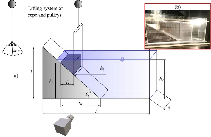
The experiments consist of sub-aerial (dry), submerged (underwater) and transitional (dry materials entering the water) sliding of a mass of granular materials on the rough and smooth inclined surfaces with different angles. Experiments are performed at the hydraulic laboratory of Polytechnique Montreal in a rectangular Plexiglas tank of length l = 0.7 m, width w = 0.15 m, and height h = 0.3 m (see Figure 4.1). An inclined plane and a sliding gate are placed inside of the tank. An initial pile of the granular material is created behind the gate at the top of the inclined plane, creating a triangular-shape reservoir with the length and height of lg and hg, respectively. Experiments are started by rapidly lifting the gate (using a rope and pulley mechanism) allowing a sudden release of the granular mass on the inclined plane. The lifting speed is approximately 1 m/s. The experiments are conducted for three regimes of (1) subaerial (dry), where the slide happens under air, (2) submerged, where the granular slide entirely happens underwater, and (3) transitional, where slide of dry material starts outside of water than granular mass enters into water. Two types of the granular materials, including the glass beads of mean diameter 0.8 mm (±0.10mm) and grain density of ρg=2.47±0.01 g/cm3, and sand of mean diameter 1.0 mm (±0.10mm) and grain density

of ρg=2.60±0.01 g/cm3. The internal friction angles are 22° and 34° (friction coefficients of 0.40

and 0.67) for the glass-beads and sand, respectively. For the submerged and transitional conditions, the tank is partially filled with an ambient fluid (i.e., the water of 20°c) with density ρw=0.998 g/cm3 and viscosity µw = 0.001 Pa.s and the height of hw (=22 and 12 cm for submerged and transitional cases, respectively).

The experimental conditions also include two slope angles (θ = 30° and 45°) and two bed roughness of smooth (Plexiglas surface) and rough, created by gluing a layer of granular material on the surface. Overall, 24 sets of experiments are conducted, with the conditions as summarized in Table 4.1. Each experiment is repeated at least three times to ensure the reproducibility of the results.

Figure 4.1 (a) Schematic and (b) photograph of the experimental

4.2.2 Experimental procedures and data acquisition

The experimental procedure consists of partially filling the reservoir with a mass of granular material to form a triangle heap of base lg height hg and width w with the initial volume fraction of around 60%. The initial dimension of the granular mass is selected to create a similar initial mass

(b)

for all experiments. The gate is lifted semi-instantaneously using a pulley-rope-weight mechanism, as shown in Figure 4.1. It releases the granular mass that spreads on the inclined plane until it reaches the horizontal surface and comes to rest. The location of the gate can be changed along the tank, allowing us to create variable reservoir size.

The quantities of interest, related to the morphodynamics and internal flow structure of the granular mass, are measured by processing the high-speed imagery data. The primary imagery data accusation tool is the Photron Mini WX-100 high-speed camera with a speed of 1080 frames per second (fps) and spatial resolution of 2048×2048 pixels. The camera has been aligned perpendicular to the side views of the granular mass. An AOS Offboard 150W flickering-free LED light source is used to illuminate the material.

4.2.3 Image processing

The goal of image processing is to extract the granular mass morphodynamic, i.e., shape, evolution, and internal flow structure (flow field). The shape and evolution of the granular mass are given by extracting the desired frames, processing the imagery data to highlight the interfaces, and digitizing the interfaces.

The flow field is extracted by the Particle Image Velocimetry (PIV) technique, providing the particle displacement and instantaneous velocity field. The PIV for granular material (also called granular PIV or G-PIV) does not require seeding, as the grains of the material can themselves act as tracer particles. It is a popular and well-tested technique (e.g., in [31, 50-52]) for extracting granular velocity field. As the granular material is not transparent, the technique can only provide the velocity field on the boundaries of the flowing mass (not inside the flowing mass).

PIV technique of this study uses the cross-correlation function of the intensity field in the image pairs (with the short time difference) to find the most probable velocities in the predetermined image subsets (called interrogation areas or windows). The tool of this study is a Matlab-based open-source code, called PIVlab [30, 68]. The accuracy of this tool for G-PIV application has been examined and proven in the past [31, 52, 68]. PIVlab uses an FFT (Fast Fourier Transform) correlation with a multi-pass deforming window algorithm to achieve accurate results. The interrogation grid is refined with every pass, and the displacement information of each pass is

stored to shift the interrogation window in the subsequent passes. This results in high spatial resolution, high signal-to-noise ratios, and high dynamic ranges [52, 68]. Here we use three passes. Before the PIV analysis, images are pre-processed with contrast limited adaptive histogram equalization (CLAHE) to enhance the image contrast.

The quality of a PIV analysis is strongly contingent on the size of the interrogation area. As a general recommendation, the size of the interrogation window should be larger than particle size and not be less than four times the maximum displacement to have a high confidence measurement [31]. The maximum particle displacement was found to be less than 2.2 pixels in all experiments. Therefore, the interrogation window for the final (third) pass is chosen equal to be 8×8 pixels (corresponding to 3.33 mm × 3.33mm in real scale). The interrogation window is selected to be 32×32 and 16×16 pixels for the first and second passes. In the captured imagery data, the diameter of particles is around 2 pixels, and the time interval between two consecutive images is selected to be 0.93 ms.

Table 4.1 Summary of experimental conditions

No. Code Regime Material Slope angle (deg) Bed roughness Dimensions (m)

lg hg h0 l0 1 D1 Subaerial (Dry) sand 30 smooth 0.08 0.04 0.2 0.34 2 D2 sand 30 rough 0.08 0.04 0.2 0.34 3 D3 sand 45 smooth 0.06 0.06 0.2 0.2 4 D4 sand 45 rough 0.06 0.06 0.2 0.2 5 D5 glass beads 30 smooth 0.08 0.04 0.2 0.34 6 D6 glass beads 30 rough 0.08 0.04 0.2 0.34 7 D7 glass beads 45 smooth 0.06 0.06 0.2 0.2 8 D8 glass beads 45 rough 0.06 0.06 0.2 0.2 9 T1 Transitional sand 30 smooth 0.08 0.04 0.2 0.34 10 T2 sand 30 rough 0.08 0.04 0.2 0.34 11 T3 sand 45 smooth 0.06 0.06 0.2 0.2 12 T4 sand 45 rough 0.06 0.06 0.2 0.2 13 T5 glass beads 30 smooth 0.08 0.04 0.2 0.34 14 T6 glass beads 30 rough 0.08 0.04 0.2 0.34 15 T7 glass beads 45 smooth 0.06 0.06 0.2 0.2 16 T8 glass beads 45 rough 0.06 0.06 0.2 0.2

Table 4.1 Summary of experimental conditions (cont’d)

4.3 Results and discussions

The results of morphodynamic and internal flow structure for various flow regimes, material type, slope angles, and bed roughness are discussed here. The dimensionless time scale of T=t / (h0/g)0.5

(free-fall timescale) has been used for the presentation of the results. The characteristic length of

h0 is the initial elevation of granular mass ( Figure 4.1), which is 20 cm and constant for all cases The vertical and horizontal length scales have been normalized using the initial dimensions of the granular mass, lg, and hg, respectively.

4.3.1 Sliding phenomenology and morphology

4.3.1.1 Impact of flow regime

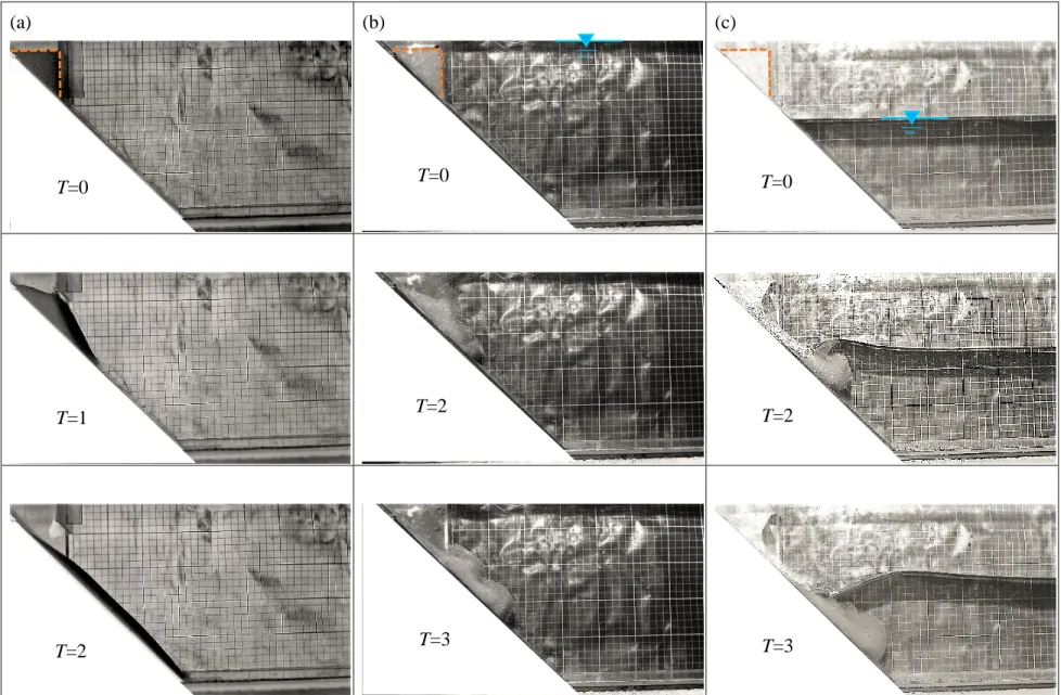
Figure 4.2 shows the snapshots of slide of glass-beads material on a 45o smooth surface for sub-aerial, submerged, and transitional slides. The surface profile has been digitized and presented in Figure 4.3. Figure 4.2a and Figure 4.3a show that for the sub-aerial slide, upon gate removal, the granular mass fails starting from front and top of the mass, then an avalanche forms and flows down the slope. The material is stretched along the slope, forming a thin uniformly distributed layer with a smooth surface. The granular assembly reaches the slope toe (at around T=2) and changes its direction. The material then slows down as the inertial force weakens and eventually comes to rest, forming a pile (with a narrow front and thick tail) at around T = 6.

17 S1 Submerged sand 30 smooth 0.08 0.04 0.2 0.34 18 S2 sand 30 rough 0.08 0.04 0.2 0.34 19 S3 sand 45 smooth 0.06 0.06 0.2 0.2 20 S4 sand 45 rough 0.06 0.06 0.2 0.2 21 S5 glass beads 30 smooth 0.08 0.04 0.2 0.34 22 S6 glass beads 30 rough 0.08 0.04 0.2 0.34 23 S7 glass beads 45 smooth 0.06 0.06 0.2 0.2 24 S8 glass beads 45 rough 0.06 0.06 0.2 0.2

For the submerged regime (Figure 4.2b and Figure 4.3b), an initial suspension of the granular material due to the gate removal mechanism is observed. The material then slides down and stretched along the slope with a round thicker front and thinner tail. A surge wave is observed at the water surface, which is propagated to the downstream. Comparing to the sub-aerial slide a slower motion, smaller velocity, and thicker frontier is observed. Furthermore, the surface of the granular mass shows material suspension and contraclockwise Kelvin-Helmholtz wave growth, which can be related to the circulation and strong shear in the water flow field near the interface. Finally, the granular mass decelerates and comes to rest after reaching down the slope. Unlike in the sub-aerial case, the final deposition of granular mass for this case has thicker front and thinner tail.

For the transitional regime (Figure 4.2c and Figure 4.3c), the evolution of the granular mass is similar to the sub-aerial case before the material enters the water body (at around T=0.8). At the impact region, the material movement slows down, which can be due to the partial saturation (resulting in a cohesion) as well as the wave impact. Then the evolution of the granular mass becomes like the submerged case. A strong surge wave also forms (at the moment of impact) and propagates downstream.

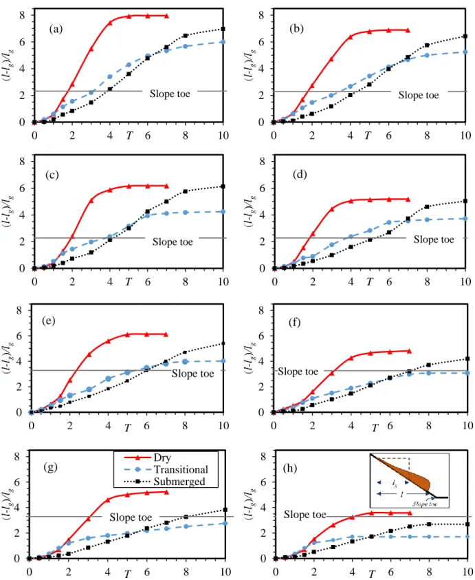
The movement and evolution of the granular mass are also quantified by plotting the dimensionless runout length (distance), defined as (l-lg)/lg. Figure 4.4 compares the time history of the runout length for various conditions. Sub-aerial cases show a S-shape curve, where one can recognize three distinctive flow regimes of (1) a short duration (T<1.5) accelerating flow regime at the initial stages, where the inertial force (driven by gravity) is larger than the resistance force, (2) a long duration steady (linear) flow, where inertial and resistance forces are in equilibrium, and (3) long-duration decelerating flow, where the resistance force is dominant. The flow reaches steady condition even on the slope surface (before the material reaches the slope toe). The material comes to rest at around T=4. Similar trend is observed for all conditions with the difference in spatiotemporal scales. It is also in agreement with the trends observed in the past studies on granular slides and slumps [38].

For the submerged case, although the three flow regimes (accelerating, steady, and decelerating) still exist, they are less distinctive as the transition between the regimes is smoother. The curve is also more stretched in time (granular mass moves almost twice slower) comparing to the sub-aerial

case. This is due to the viscous resistance force of the water phase. The transitional case is, however, present a more complex runout length time history. While the three flow regimes still exist, the additional deceleration and reacceleration can be observed, at and after the granular mass enters the water body. The deceleration can be due to the wave impact as well as the increase in the cohesion and yield stress (as the result of the partial saturation) at the moment of entry. The granular mass reaccelerates, once it becomes fully saturated (resulting in a large decrease in the cohesion and yield stress). The reacceleration can happen even after material passes the slope toe and reach the horizontal surface. Comparing to the submerged case, one can observe that granular mass initially moves faster than the submerged condition, but the latter falls behind. A smaller final runout length is observed for the transitional case comparing to that of the submerged case. The time scales are however similar (T ~6 to 7) and almost twice longer than the sub-aerial case.

Figure 4.2 Snapshots of slide of glass-beads material on a 45° smooth surface. (a) Sub-aerial slide (case D7) , (b) Submerged slide (case S7) and (c) Transitional slide (case T7)

T=0 T=0 T=0 T=2 T=3 T=1 T=2 T=2 T=3

Figure 4.2 Snapshots of slide of glass-beads material on a 45° smooth surface. (a) Sub-aerial slide (case D7) , (b) Submerged slide (case S7) and (c) Transitional slide (case T7) (cont’d)

T=4 T=5 T=8 T=3 T=4 T=6 T=4 T=5 T=8

(a)

(b)

(c)

Figure 4.3 Time sequences of slide of glass-beads material on a 45° smooth surface. (a) Sub-aerial slide (Case D3), (b) Submerged slide and (c) Transitional slide

0 2 4 0 2 4 6 8 1 0 y/ hg x/l_g T = 0 T = 1 T = 1.5 T = 2 T = 3 T = 4 T = 5 0 2 4 0 2 4 6 8 1 0 y/ hg x/l_g T = 0 T = 1 T = 2 T = 4 T = 5 T = 6 T = 7 T = 8 T = Final 0 2 4 0 2 4 6 8 1 0 y/ hg x/l_g T = 0 T = 1 T = 2 T = 4 T = 5 T = 6 T = 7 T = Final

4.3.1.2 Impact of the material type, surface roughness, and slope angle

Comparing the runout distances (Figure 4.4) for two surface roughness, one can observe a shorter runout distance for the rough surface (Figure 4.5 highlights this for the sub-aerial case). This difference is less significant for the submerged and transitional cases (esp. for the 45° slope), the presence of water reduces the normal force of granular mass on the sliding surface and also act as a lubricant, resulting in less friction. The runout time scale is, however, close for the rough and smooth surfaces. Impact of material is more significant than the roughness. Sand material (with 1.68 times higher friction coefficient) has resulted in a shorter runout length and duration comparing to the glass-beads. Again, such impact is less significant for the submerged and transitional cases (esp., for the 45° slope).

The higher slope has larger runout distance and shorter runout duration as the result of higher inertial force (driven by gravity) and smaller resistance force. For the 30° slope the material barely reaches slope toe, particularly for the submerged and transitional cases. Furthermore, for this angle, the duration of the steady flow regime is shorter. While for the 30° slope, the effects of roughness and material type are visible from the beginning, for the 45° slope such effects are only present at later times, in the middle of the steady flow regime (T>2 for sub-aerial cases). In other words, the higher initial acceleration of 45° slope, reduces the impact of the roughness and material type. This can be due to the fact that the 45° slope angle is higher than the friction angle of both sand and glass-bead, while the 30° slope is only higher than the friction angle of glass-beads. This can impact the yield stress and the initial failure of the material.

Figure 4.4 Comparison of the normalized runout length for 45° granular sliding with (a) glass beads and smooth surface, (b) glass beads and rough surface, (c) sand and smooth surface, (d)

0 2 4 6 8 0 2 4 6 8 10 ( l-lg )/l g T Slope toe (a) 0 2 4 6 8 0 2 4 6 8 10 ( l-lg )/l g T Slope toe (b) 0 2 4 6 8 0 2 4 6 8 10 ( l-lg )/l g T Slope toe (c) 0 2 4 6 8 0 2 4 6 8 10 ( l-lg )/l g T Slope toe (d) 0 2 4 6 8 0 2 4 6 8 10 ( l-lg )/lg T Slope toe (e) 0 2 4 6 8 0 2 4 6 8 10 ( l-lg )/lg T Slope toe (f) 0 2 4 6 8 0 2 4 6 8 10 ( l-lg )/l g T Dry Transitional Submerged Slope toe (g) 0 2 4 6 8 0 2 4 6 8 10 ( l-lg )/l g T Slope toe (h)

sand and rough surface, and 30° sliding with (e) glass beads and smooth surface, (f) glass beads and rough surface, (g) sand and smooth surface, (h) sand and rough surface.

Figure 4.5 Comparison of the normalized runout length of dry (sub-aerial) granular sliding of (a) 30° slope angle, and (b) on 45° slope angle.

4.3.2 Internal flow structure

This section provides the velocity field extracted using the G-PIV technique for the sub-aerial and submerged conditions. Figure 4.6 presents the snapshots of velocity vector fields of subaerial sliding of glass beads on a smooth surface with the inclination angle of 30° (case D5). To enhance the quality of the velocity vector fields’ appearance, all vectors have been smoothed, and the autoscale procedure has been applied. The velocity vectors outside of the granular assembly are due to the initial suspension of some particles caused by the gate removal process. At the initial stages, a yielded region near the granular surface and front and a non-yielded region (with near-zero velocity) near the slope surface can be recognized. The yielded region gradually grows and is extended to whole granular mass forming a uniform layer of granular particles on the surface of the slope.

Figure 4.7a shows an instantaneous profile of velocity component tangent to the slop at T=3 (within the steady flow period) for sub-aerial case D5. It has been plotted for a section at the middle of the slope and perpendicular to it. This figure also provides a comparison with an unsteady viscoplastic

0 2 4 6 8 10 0 2 4 6 8 ( l-lg )/l g T Glass - Smooth Sand - Smooth Glass - Rough Sand - Rough 0 2 4 6 8 10 0 2 4 6 8 ( l-lg )/l g T

Glass beads - Smooth Glass beads - Rough Sand - Smooth Sand - Rough

(b) (a)

theory, which will be discussed in the next section. A well-developed and relatively logarithmic velocity profile with the maximum velocity (of 0.84 m/s) at the surface is observed. A shear layer (with a smooth velocity transition across the layer) is also observed at around h=0.008 m. The velocity of the center of mass has been provided in Figure 4.7b. One can see an accelerating (for

T<3) and constant (for T>3) velocity. This agrees with the runout length (Figure 4.4), although

with a delay (as the runout length is for the frontier not the center of mass).

Submerged regime shows a different flow pattern. As Figure 4.8 shows for a 45° submerged case (case S7), the initial yielded and non-yielded regions are less distinctive at the initial steps. Strong counterclockwise circulations are also observed (esp. near the front) due to the water shear. The velocity profile in Figure 4.9a shows a logarithmic profile (with the maximum velocity of 0.2 m/s) near the bed and a negative velocity of 0.3 m/s (due to the circulation back-flow) near the granular surface. Time history of the center of mass velocity of the center of mass Figure 4.9b) shows an initial acceleration followed by a constant velocity, similar to the sub-aerial case but with much smaller velocity magnitude.

Figure 4.10 shows that the flow field of the transitional regime is similar to that of the sub-aerial regime (for the materials outside of water) and submerged regime (for the materials inside of water). The interesting part, however, is the region near the water surface, where a dramatic velocity decrease (due to partial saturation) is observed inside and outside of water.

T=0.5 T=1 T=2

(a)

(b)

Figure 4.7 Experimental and theoretical (a) velocity profile at T=3 and (b) time history of the center of mass velocity for the sub-aerial case D5.

T=1 T=2 T=4

(a)

(b)

Figure 4.9 Experimental and theoretical (a) velocity profile at T=3 and (b) time history of the center of mass velocity for the submerged case S7.

0 0.025 0.05 -0.5 -0.25 0 0.25 0.5 h (m ) V (m/s) h 0 0.1 0.2 0.3 0.4 0 1 2 3 4 5 V C OM (m /s) T Experimental Theory

Figure 4.10 G-PIV velocity vectors (left) and velocity magnitude field (right) for a transitional slide (case T7) at the moment of impact (T=2). The dashed and dotted lines show approximate

water and granular surfaces, respectively.

4.4 Theoretical models

4.4.1 Sub-aerial condition

In recent years, substantial theoretical progress [57, 58] have been made for granular. Those approaches consist in describing the granular medium as an incompressible fluid whose behavior is captured by a viscoplastic local rheology that can be used to write the stresses in the momentum equations: D Dt  u=  +σ g (1) p = − + σ Ι τ (2)

where σ is the Cauchy stress tensor, u is the velocity vector, p is the pressure, τ the deviatoric part of the stress tensor, I is unit tensor, and ρ is the bulk density. For the flow motion down an inclined plane, which is assumed to be monodirectional flow (along the slope) with the uniform thickness (as shown in Figure 4.11) the momentum equation becomes:

Low velocity

region