© Amandine Pierre, 2020
Ajustements du biais de mesure de précipitation solide
et effets sur les bilans hydrologiques en milieu forestier
boréal
Thèse
Amandine Pierre
Doctorat en sciences forestières
Philosophiæ doctor (Ph. D.)
A
JUSTEMENTS DU BIAIS DE MESURE DE PRÉCIPITATION SOLIDE ET
EFFETS SUR LES BILANS HYDROLOGIQUES
EN MILIEU FORESTIER BORÉAL
Thèse de doctorat
Amandine PIERRE
Sous la direction de :
Sylvain JUTRAS, directeur de recherche
François ANCTIL, codirecteur de recherche
ii
Résumé
Ce travail est la fusion de deux projets de recherche complémentaires et contribue à l'approfondissement des connaissances dans les domaines des mesures de précipitation solide et dans la stratégie de modélisation hydrologique en milieu forestier boréal. Toutes les données utilisées pour ces travaux proviennent de la forêt Montmorency, qui est la forêt d’enseignement et de recherche de l’Université Laval située à Québec.
Les incertitudes liées aux simulations des débits des bassins versants par les outils de modélisation hydrologiques dépendent du choix du modèle considéré, mais sont aussi liées à la qualité des données météorologiques entrantes. Il est question ici de tout d’abord quantifier les incertitudes reliées aux mesures de précipitation solide, ensuite proposer une méthode d’ajustement novatrice, et enfin une stratégie de modélisation hydrologique en milieu forestier boréal. L’élaboration d’une base de données météorologique regroupant 15 types de précipitomètres, dont deux référents mondiaux, a été réalisée grâce notamment à la mise en place du site météorologique Neige, déployé depuis 2014. Concernant les incertitudes des mesures liées au phénomène de sous-captation de précipitation solide, des approches déterministes historiques de débiaisage des données sont tout d’abord évaluées. Les résultats démontrent un biais initial moyen d’environ 30%, et une surestimation rémanente des quantités de précipitation après ajustement. Une approche probabiliste est ensuite proposée, et les résultats montrent un biais moyen divisé par 5 après application de la méthode. Enfin, des analyses de sensibilités des paramètres des modèles hydrologiques ainsi que de leurs performances face aux variations des données de précipitation solide sont réalisées sur un ensemble de 20 modèles conceptuels à partir de la base de données hydrologique du bassin versant appelé le Haut-Montmorency. Cette étude permet finalement de mettre en évidence que le biais de mesure d’équivalent en eau du manteau nival pourrait influencer la qualité des bilans hydriques des bassins versants dans certaines conditions. Ainsi, une analyse de sensibilité des modèles hydrologiques rigoureuse a permis de mettre en évidence qu’un ajustement des données de précipitation solide est nécessaire en amont de la calibration conjointement à l’utilisation des modèles. L’originalité de ces travaux dépend principalement de l’exceptionnalité des sites d’études mais aussi de la qualité du travail des techniciens en observation météorologique et la coopération d’un grand nombre de partenaires privés et publics.
iii
Abstract
This work joins two complementary research projects and contributes to improve the knowledge on solid precipitation measurements and hydrological modelling strategy in the boreal forest environment. All the data used in this work comes from the Montmorency Forest, which is the teaching and research forest of Université Laval located in Quebec.
The uncertainty related to flows forecast by hydrological models depends on the choice of the model, but are also linked to the quality of incoming meteorological data. This work aims first to quantify uncertainties related to solid precipitation measurements, then to propose an innovative method of adjustment and finally to establish a hydrological modelling strategy for the boreal forest environment. The development of a large meteorological database, including data from two world reference instruments, was done thanks to the Neige site deployed since 2014. Regarding uncertainties related to the solid precipitation undercatch phenomenon, five deterministic approaches from the literature are first evaluated. Results show that the initial bias is 30% on average and there is still an overestimation of the solid precipitation quantity after a deterministic adjustment. A probabilistic approach is developed and results show that the bias is divided by 5 on average. Finally, sensitivity analysis of hydrological models’ parameters, and their performance facing different solid precipitation quantities, is done on a set of 20 conceptual models based on the hydrological database of the catchment area called the Haut-Montmorency. This study highlights that the snow water equivalent measurement bias of the snowpack could influence the quality of water balances in the catchment under certain conditions. A deep sensitivity analysis of hydrological models showed that an adjustment of the solid precipitation was required prior to their calibration. The originality of this thesis depends on the exceptional studied sites, the quality of technicians work and the collaboration of numerous public and private partners.
iv
Table des matières
Résumé ... ii
Abstract ... iii
Table des matières ... iv
Liste des figures, tableaux, illustrations ... vii
Remerciements ... xi
Avant-propos ... xii
INTRODUCTION GÉNÉRALE ... 1
Chapitre 1: Évaluation d’équations de transfert de mesures de précipitations solides pour des précipitomètres sans paravent et avec paravent de type simple Alter ... 7
Résumé ... 8
Abstract ... 9
1.1. Introduction ... 9
1.2. Material and methods ... 11
1.2.1. The Neige site ... 11
1.2.2. Transfer functions ... 14
1.2.3. Geographic, climatic and meteorological characteristics of the studied sites ... 19
1.2.4. Precipitation measurements ... 19
1.2.5. Selection of twice-daily solid precipitation events ... 20
1.2.6. Evaluation procedure ... 21
1.2.7. Recalibration of the parameters ... 22
1.3. Results ... 22
1.3.1. Event selection ... 22
1.3.2. PCA results ... 22
1.3.3. Gauge data correlations ... 23
1.3.4. Evaluation of the catch efficiency transfer functions at the Neige site ... 24
1.3.5. Recalibration of catch efficiency transfer functions using the Neige site dataset ... 29
1.4. Discussion ... 30
1.4.1. Distribution of the raw CE data ... 30
v
1.4.3. Hourly and twice-daily adjustment ... 32
1.4.4. Temperature effect ... 33
1.4.5. Recalibration of the parameters ... 33
1.4.6. High and low wind speed effect ... 34
1.4.7. Climate and wind speed impact ... 34
1.4.8. Unshielded and single-Alter-shielded precipitation adjustment ... 35
1.4.9. Total quantity of precipitation and hydrological relevance ... 36
1.5. Conclusion ... 36
Acknowledgements ... 38
Chapitre 2: Une approche probabiliste pour l’évaluation de l’efficacité des paravents dans le cadre de la mesure de précipitation solide ... 39
Résumé ... 40
Abstract ... 41
2.1. Introduction ... 42
2.2. Material and methods ... 44
2.2.1. Data collection and validation... 44
2.2.2. Data analysis ... 49
2.2.3. Adjustments on partial dataset: cross-calibration ... 52
2.3. Results ... 53
2.3.1. Parameter identification ... 53
2.3.2. Shield ranking according to CE at mean Wind speed ... 54
2.3.3. Cumulative unadjusted and adjusted time series ... 55
2.3.4. Bias of unadjusted and adjusted end of season totals ... 56
2.3.5. Distribution of unadjusted and adjusted series ... 56
2.3.6. Cross-calibration results ... 58
2.4. Discussion ... 59
2.4.1. Mean K (μ) ... 59
2.4.2. Standard deviation K (σ) ... 61
2.4.4. Probabilistic adjustment of snow catch ... 61
2.4.5. A tool for operational hydrology... 62
2.5. Conclusion ... 62
vi
Chapitre 3: Évaluer la sensibilité des modèles hydrologiques en réponse à des variations de quantité de
précipitation solide pour un bassin forestier de type boréal ... 65
Résumé ... 66
Abstract ... 67
3.1. Introduction ... 68
3.2. Material and methods ... 69
3.2.1. Hydrometeorological data ... 70
3.2.2. Hydrological modeling ... 72
3.3. Results and discussion ... 75
3.3.1. General description of the KGE results ... 75
3.3.2. Detailed description of KGE components ... 76
3.3.2. Parameters values of the model(s) and elasticity ... 79
3.3.3. Spring hydrograms ... 80
3.4. Conclusion ... 81
Acknowledgements ... 82
CONCLUSION GÉNÉRALE ... 83
vii
Liste des figures, tableaux, illustrations
Figures
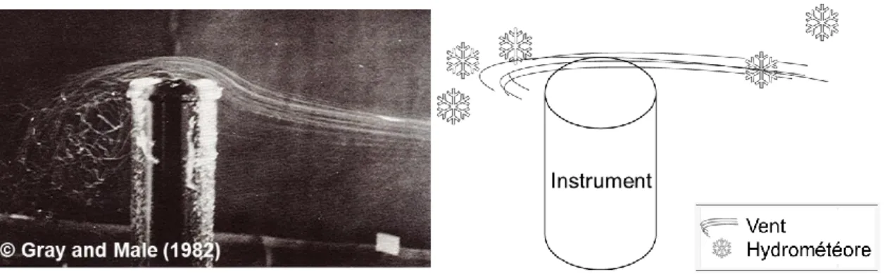
Figure I. Illustration du phénomène de sous-captation, à gauche, photographie extraite de Gray & Male (1982), à droite une schématisation du phénomène.
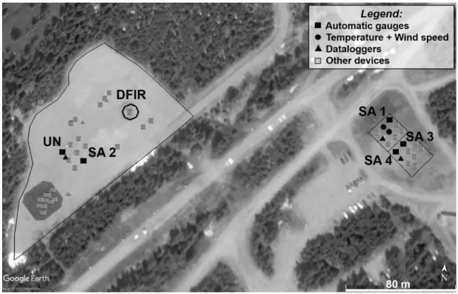
Figure 1.1: Map of the Neige site and location of the automatic and manual sensors used in the present study (black) and other devices (grey).
Figure 1.2: Map of the SPICE sites used in this study, overlaying the Köppen-Geiger climate classification (Kottek et al. 2006; Rubel et al. 2017).
Figure 1.3: Picture of a) DFIR and Tretyakov shield fencing an H&H90 manual weighing gauge ; b) Single-Alter-shielded Geonor T-200B ; c) Unshielded OTT Pluvio².
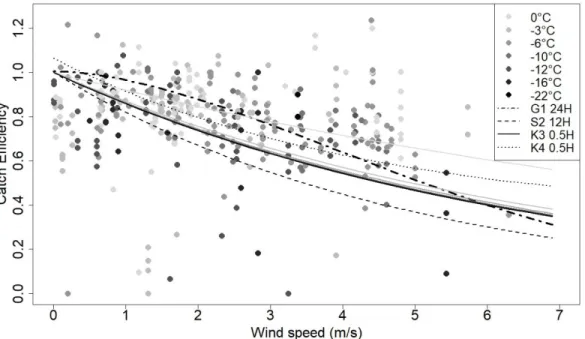
Figure 1.4: a): Individuals factor map (PCA) from all the study sites and three virtual sites of G1 24H, S2 12H and K3 & K4. Virtual S2 12H*: Only Bratt’s Lake site) regarding the climate (Kottek et al. 2006), the mean Tair (°C), annual solid P (mm) and mean Ugh (m s-1) variables. A colored point highlight the virtual and Neige sites. (b): Variable factor map (PCA) from all the variables used to build the PCA. Figure 1.5: Catch efficiency transfer functions and CE from selected twice-daily solid precipitation events for the unshielded gauge at various wind speeds. Temperature is represented by different shades. Dotted-point line: equation G1 24H; Full line: equation K3 0.5H with different shades representing different temperatures; Dot-dashed line: equation K4 0.5H.
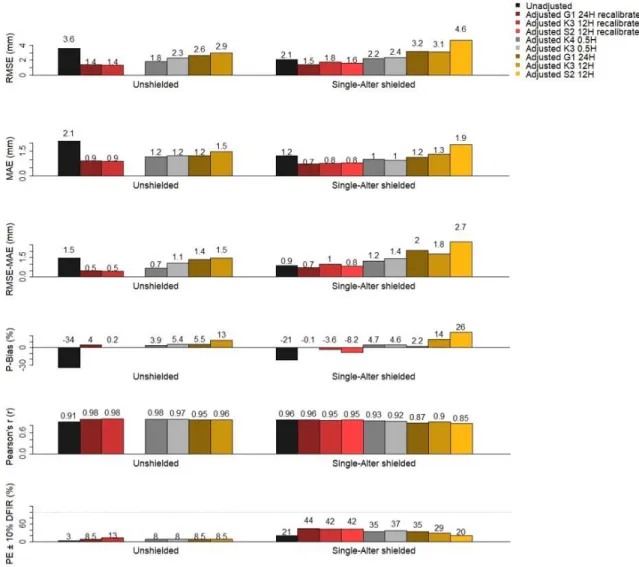
Figure 1.6: Catch efficiency transfer functions and CE from selected twice-daily solid precipitation events for single-Alter-shielded instruments at various wind speeds. Temperature is represented by different shades. Dot-dashed line: equation G1 24H; dashed line: equation S2 12H; full line: equation K3 0.5H with different shades representing different temperatures; dotted line: equation K4 0.5H. Figure 1.7: Comparison of statistics describing unadjusted and adjusted twice-daily solid precipitation events using raw parameters or recalibrated parameters for unshielded, and single-Alter-shielded measurements. RMSE, MAE, RMSE-MAE, P-bias, Pearson’s cc. (the Pearson correlation coefficient), and PE ±10% DFIR (the percent of events that were within ±10% of the DFIR reference) are shown.
viii
Figure 2.1: Map of location of the Neige site at Forêt Montmorency, Eastern Canada. (Extract from Google Earth, author Amandine PIERRE)
Figure 2.2: Photography of manual massic H&H90 gauge in a Tretyakov shield and a DFIR, Neige site, winter 2017, author Amandine PIERRE
Figure 2.3: Algorithm diagram used for snow event selection
Figure 2.4: Example of different distribution of 7 adjustment multiplier (K) Single-Alter shielded instrument data centered on their mean wind speed. Black line is the normal law adjusted to the data. Figure 2.5: Mean K (μ) and standard deviation K (σ) (variability) as a function of wind speed during the event (Equations 1 and 2) for the various devices. The vertical grey dotted line identifies the mean wind speed during the 2014-2018 solid precipitation events at the Neige site (2.2 m s-1).
Figure 2.6: Typical graphic of cumulated solid precipitation measurement (mm SWE) of DFIR, Pluvio² SA4, and 50 Pluvio² SA4 adjusted events during winter 2018.
Figure 2.7: Histogram of bias of total solid precipitation measured by the DFIR (mm SWE) at the end of winters and unadjusted and adjusted data aggregated by type of windshields; ± s.d. values. Figure 2.8: Boxplot of unadjusted and (probabilistic) adjusted CE.
Figure 2.9: (left) Adjustment made on raw data of K values and result of adjustments made on (middle) mean K (μ)and (right) standard deviation K (σ) from the calculated sliding windows as a function of mean wind speed during the sub-event for unshielded and typical shielded (Single-Alter) devices. Figure 2.10: Distribution of the Pa, Pb, Pc, La and Lb free parameter values following a k-fold analysis. Red “o” localise the respective values from Table 2.2.
Figure 3.1: Map of location of the Montmorency Forest, Eastern Canada.
Figure 3.2: Map of location of the Haut-Montmorency catchment and the meteorological ECCC and MFFP stations.
Figure 3.3: Hydrological model performance in terms of the modified Kling-Gupta Efficiency (KGE’) and its components (r the correlation coefficient, β the bias and γ the variability ratio) against snow adjustments. Boxplots contain the 20 hydrological models. The period of simulation considered is indicated in parenthesis (Cal. = Calibration ; Val. = Validation).
ix
Figure 3.4: Normalized parameter values of all hydrological models regarding the different solid precipitation data as input for calibration. The “Min.” and “Max.” of the boxes illustrates the upper and lower calibration boundaries of the respective models. The two most right parameters in each subplots are the snow accounting routine CemaNeige free parameters. The color scale ranging from red to dark blue indicates increasing solid precipitation adjustment (red = - 25%, dark blue = + 50%).
Figure 3.5: Typical examples of hydrograms produced with Hydrological model 11. Simulations obtained from unadjusted input are drawn in black, while the 15 simulations obtained from adjusted input series are represented by a color gradient ranging from red to dark blue (which correspond to -25 % and +50 % solid precipitation adjusted respectively).
x
Tables
Table 1.3: Configuration of the precipitation gauges installed on the Neige site. Table 1.1: Geographic, climatic and meteorological characteristics of the study sites.
Table 1.2. Original and recalibrated parameter values of the 5 equations used in this study for unshielded (UN) and Single-Alter-shielded (SA) instruments
Table 1.4: Results of intercomparison between twice-daily precipitation events measured by single-Alter-shielded gauges on the Neige site.
Table 1.5: Error statistics for transfer functions from the literature and recalibrated transfer functions. (*). +, - or = : criterion is improved, respectively worse or the same, after the use of the transfer function compared to the unadjusted data. |P-bias| is the absolute P-bias.
Table 2.1: List of Neige precipitation gauges available to the study.
xi
Remerciements
J’aimerais remercier mon directeur Sylvain Jutras et codirecteur François Anctil pour avoir eu la force, le courage et surtout (surtout) la patience de m’accompagner tout au long de cette épreuve. Je vous souhaite plein de merveilleux diplômés à suivre. Il m’est important aussi de remercier l’ensemble de mes coauteurs Craig Smith, John Kochendorfer, Vincent Fortin ou Antoine Thiboult pour leurs merveilleux apports à mes travaux ainsi que pour leur soutien moral.
Il est primordial de remercier une fois de plus ici, on ne le fait jamais assez, les observateurs météo ainsi que l’ensemble des intervenants de la forêt Montmorency : Robert Coté, Charles Villeneuve, Gilles Bilodeau, Sylvain Tanguay, Francois Richard, Pierre Martin Marotte, Pierre Vaillancourt, Julie Bouliane, Patrick Pineault, Hugues Sansregret... Un énorme merci à vous, sans votre coopération ces travaux n’auraient pu aboutir.
Un merci aussi à tous les partenaires, sans qui la construction du site Neige et son entretien n’aurait pu se faire et/ou qui m’ont donné l’accès à leur données et partagé leur expérience : Environment and Climate Change Canada (ECCC), le Ministère de l’Environnement et de la Lutte contre les Changements Climatiques (MELCC), Campbell Sci (Richard Laffin, the one), Geonor Inc., Université Sherbrooke, Institut national de la Recherche Scientifique (INRS), HydroQuébec, Rio Tinto Alcan, le Ministère des Forêts, de la Faune et des Parcs (MFFP). Votre contribution pour la pérennité du site est fortement appréciée. Aussi, je remercie tous ces flocons qui, s’ils n’étaient pas tombés du ciel, n’auraient pu faire partie intégrante de cette thèse. Merci à ceux qui sont tombés dans les buckets, merci à ceux qui ne sont pas tombés dans les buckets, merci à ceux qui sont tombés sur les touches de l’ordinateur qui faisait ses mises à jour Windows régulières, merci à ceux qui m’ont gelé les doigts parfois jusqu’au sang, merci à ceux qui sont tombés dans ma bouche lorsque je tombais de mon échelle, merci à ceux qui se sont empilés sur le skidoo jusqu’à l’immobiliser, merci à ceux qui se sont immiscés dans les cadenas. Flocons, je vous aime.
Enfin, comme il se doit, un énorme merci à tous les partenaires de lab qui m’ont accueillie « chaleureusement » à mon arrivée au mois de novembre puis ceux qui ont pris la relève: Phil, Lelia, Sarah, Roxanne, Stéphanie, Karelle… Un merci à la famille pour leur soutien moral (Merci Maman, Papa et Yannick !) Un GROS merci à tous les potos pour leur patience face à mes (peu nombreux) chialages et mes histoires (souvent courtes) : Nilliiie, Ricardo, Mel, André, Caro, Tibo, Léa, Élise, Léo, Anne F, Dadou, Manon, Cake, Vilmantas, Alex… Un merci particulier à celui qui m’a peut-être le plus endurée cette dernière année, ça fait long l’attente de la bouteille de champagne quand même, Guillaume.
xii
Avant-propos
C’est avant tout le libre accès à l’ensemble de toutes les bases de données, ainsi que l’implication et la coopération de l’ensemble des partenaires, qui ont permis le bon cheminement et enfin l’aboutissement de ces travaux de doctorat.
1
I
NTRODUCTION GÉNÉRALE
De 1995 à 2015, les inondations représentaient près de la moitié des catastrophes naturelles recensées dans le monde, affectant 2.3 millions de personnes, et faisant 242 000 victimes (Wahlstrom and Debrati, 2015). Conséquent à un déluge de 200 à 350 mm de précipitations en trois jours, le débordement de la rivière Bow et de ses tributaires a couté plus de 6 milliards de dollars, et provoqué le déplacement de plus de 100 000 personnes en 2013. Cet évènement fut considéré comme la catastrophe naturelle la plus couteuse de l’histoire du Canada (Pomeroy et al., 2015). Les inondations, plus ou moins prévisibles, sont le sujet d’étude de nombreux modèles hydrologiques (Fortin et al., 2001 ; Fassnacht 2007 ; Viatgé et al., 2012), économiques (Smith, 1994) ou encore hydro-économiques (Duttaa et al., 2003). Les modèles hydrologiques, qui ne sont pas uniquement restreints à l’étude des phénomènes de crue mais intègrent généralement l’ensemble des dynamiques hydrologiques des bassins versants, sont reconnus comme générant épisodiquement des prévisions incertaines (Beven and Binley, 1992 ; Andréassian et al., 2001 ; Gupta et al., 2009). Aussi, dans les écosystèmes boréaux, il s’avère que l’accumulation de la neige en hiver puis sa fonte au printemps contribue aux débordements des cours d’eau à cette période (Burn et al., 2016). Or, il est connu que les mesures des précipitations solides sont elles aussi associées à des incertitudes non négligeables (Goodison et al., 1998 ; Smith 2009 ; Rasmussen et al., 2012 ; Kochendorfer et al., 2017).
Une incertitude majeure connue, liée aux mesures de précipitation solide par les instruments météorologiques usuels, concerne principalement le phénomène de la sous-captation. Le phénomène de sous-captation de précipitation solide résulte de la création d’un micro tourbillon à l’orifice du précipitomètre, dû aux turbulences de vent, et qui provoque une accélération et un déplacement des hydrométéores, ici les flocons, autour du récipient (Rasmussen et al., 2012). Ceux-ci ne sont ainsi pas mesurés et l’évènement de précipitation est alors sous-estimé de manière quantitative. Ce phénomène est illustré par la Figure I. ci-dessous :
2
Figure I. Illustration du phénomène de sous-captation, à gauche, photographie extraite de Gray & Male (1982), à droite une schématisation du phénomène.
Il a été démontré que la vitesse du vent ainsi que l’intensité des turbulences (Rasmussen et al., 2012 ; Hertig and Spiess, 1991) sont les facteurs perturbateurs principaux de la mesure de précipitation solide. Aussi, il apparaitrait que la taille et la nature des flocons, eux-mêmes liés aux conditions de température et d’humidité du milieu, influenceraient la captation de la précipitation par les instruments (Thériault et al., 2012). Par ailleurs, la forme des orifices des récipients utilisés (Hertig and Spiess, 1991), le type de matériaux de surface constituant l’instrument (Devine and Mekis, 2008) ou même le type de paravent entourant celui-ci (Rasmussen et al., 2012) induirait une variation significative de la captation de précipitation par les précipitomètres.
Les mesures de précipitation solides existent depuis au moins le 19e siècle (Symons, 1888). À leurs débuts, les mesures effectuées étaient des relevés manuels. Ainsi, il apparait que les protocoles et que la qualité de l’observation manuelle ait été éprouvés au moins un siècle avant l’apparition des premiers appareils de mesure automatiques. De ce fait, elle a constitué la référence en matière d’évaluation des premiers instruments automatiques (Goodison, 1978). Un instrument de référence est considéré comme mesurant le « true snowfall » (Yang et al., 1993) et permet de quantifier un biais dans la mesure de précipitation solide, constituant ainsi le point de départ des stratégies d’ajustement. D’après les travaux de Rasmussen et al. (2012), il est apparu que la qualité d’observation des instruments automatiques présentait une variabilité plus forte que celle de l’observation manuelle. Les auteurs ont démontré que ceci était lié tout d’abord au phénomène de « capping » qui est le fait qu’une certaine quantité et qualité de neige soit capable de recouvrir complètement l’orifice de l’instrument, formant ainsi un capuchon et bloquant les mesures jusqu’à sa fonte. Ceci induit un biais et un délai avec l’observation réelle des évènements de précipitation. D’autre part, il se pourrait que l’accumulation
3
de neige autour de l’instrument automatique, et donc son changement de forme variable, pourrait aussi avoir une influence sur la précision des mesures de précipitation (Hertig and Spiess, 1991) et expliquer la plus grande variabilité de ses mesures. Ces deux phénomènes ne concernent pas les observations manuelles car l’observateur en météorologie effectue un nettoyage journalier, ou bi-journalier, systématique de ses instruments. Ainsi, lorsque les conditions financières sont favorables, la mesure manuelle constitue encore aujourd’hui la référence préférentielle en matière de mesure de précipitation solide (Mekonnen et al., 2015 ; Milewska et al., 2018 ; Pierre et al., 2019). Les instruments à relevé manuel équipés de type Double Fence Intercomparison Reference (DFIR) (Metcalfe and Goodison, 1993 ; Yang et al., 1993) ou d’un paravent de type buisson (Bush-gauge) (Golubev, 1989) présentent notamment des résultats de captation supérieurs aux instruments automatiques (Nitu and Wong, 2010) et sont considérés comme des paravents de référence mondiale par le World Meteorological
Organization (WMO). Cependant, depuis le début des années 2000, les programmes nationaux de
surveillance du climat automatisent les stations à l’aide d’appareils de mesure standards comme le Geonor T-200B (Geonor Inc., Oslo, Norvège) ou l’OTT Pluvio² (OTT Hydromet, Kempten, Allemagne), par exemple, munis de paravents ou non. Ainsi, un nouveau type de d’appareil de référence mondiale a pu voir le jour : le Double Fence intercomparison Automated Reference (DFAR) qui n’est autre qu’un DFIR automatisé. Ceci permet, entre autres, de considérer les évènements de précipitation à une échelle temporelle plus précise que celle de la demi-journée (Kochendorfer et al., 2018 ; Smith et al., 2019). Or, certaines études démontrent que les appareils de mesure automatiques standards sous-estime entre 20 et 50% de la précipitation lors d’un évènement météorologique (Goodisson, 1998 ; Kochendorfer et al., 2017b ; Smith, 2009 ; Rasmussen et al., 2012).
Dans un premier chapitre, le phénomène de sous-captation est analysé et quantifié grâce aux données de terrain récoltées sur le site Neige de 2015 à 2018. Ce site est localisé à la forêt Montmorency, au cœur de la forêt boréale québécoise. Cette forêt est un territoire de recherche attribué à l’Université Laval depuis 1965. Comparativement à des zones tempérées, l’impact du phénomène de sous-captation de précipitation solide s’amplifie en milieu boréal où l’hiver peut durer 6 mois de l’année, et où la proportion de précipitation sous forme solide est majoritaire durant cette période et où l’équivalent en eau (EEN) du manteau nival est conséquent. L’hypothèse de travail de ce premier axe est ainsi de valider si la quantification de ce phénomène sur le site d’étude est réalisable et s’il est possible de proposer des ajustements de précipitation solide optimaux. Le site Neige est en place depuis 2014 et regroupe au total plus d’une cinquantaine d’appareils de mesure météorologiques usuels incluant
4
plusieurs combinaisons de précipitomètres et de paravents, de même que les deux instruments de référence mondiale à relevé manuel cité précédemment : le DFIR et le Bush-gauge. Des équations de transfert déterministes, c’est-à-dire apportant une solution unique (Yevjevieh, 1987), issues de la littérature, sont appliquées sur les données du site d’étude et constituent ainsi une première stratégie dans l’ajustement des données de précipitation solide. La qualité de l’ajustement a été évaluée grâce aux mesures issues des instruments de référence. Ceci a permis de mettre en évidence la rémanence d’un biais dans les données ajustées et donc la remise en question partielle de cette approche déterministe. À plus forte raison, ce biais peut se cumuler et croître tout au long de l’hiver, ce qui perturberait d’autant plus les bilans en eau du manteau nival ainsi que les bilans hydrologiques à sa fonte au printemps, et ce, particulièrement en milieu boréal où les précipitations solides sont fréquentes. Ces résultats constituent un article publié dans le Journal of Atmospheric and Oceanic
Technology (American Meteorological Society) en 2019.
Le deuxième chapitre de ce manuscrit propose une nouvelle stratégie d’ajustement du biais de mesures de précipitation solide, de type probabiliste, développée afin d’ajuster les données de précipitations tout en conservant l’incertitude inhérente aux instruments et aux caractéristiques du site d’étude (Pierre et al., 2019). Les travaux de Terink et al. (2010) mesuraient l’incertitude liée aux mesures de précipitation de plusieurs stations météorologiques à l’échelle d’un territoire donné. Il proposait ainsi, non plus une série moyenne de précipitation sur le territoire, mais un ensemble de séries de précipitations possibles qui reflétaient au plus proche de la réalité la donnée de précipitation. À une échelle réduite à celle du précipitomètre uniquement, ces travaux ont inspiré l’approche novatrice de ce deuxième chapitre dont l’hypothèse est de valider si la moyenne et la variance (incertitude) de l'erreur liée aux mesures d'un instrument augmentent avec la vitesse du vent. Il s’agit ici d’exprimer un indice de l’efficacité de captation des instruments comparativement aux instruments de référence (qui varie de 1 à +∞), des différents couples instrument-paravent en fonction de la vitesse du vent. Ensuite ces données sont parcourues par une fenêtre glissante qui, à chaque arrêt, extrait la moyenne et l’écart-type de l’erreur. Des équations de transfert déterministes usuelles (Goodison et al, 1998) ont ensuite été ajustées sur les moyennes de l’indice d’efficacité de captation, tandis que des équations linéaires ont été ajustées sur les écarts-types de ces mêmes indices. Un ajustement probabiliste (d'ensemble) des mesures de précipitations solides est alors possible puisqu’il peut tenir compte de la variance inhérente des relevés d’observation. Une approche de calibration croisée a été réalisée, en sélectionnant aléatoirement une partie du jeu de données, en calibrant les paramètres des équations
5
sur ce jeu de données et ensuite en réitérant cette étape jusqu’à ce que le jeu de données ait été sélectionné une fois au complet. Ceci permet de mettre en évidence la stabilité de tous les paramètres polynomiaux calibrés, mais aussi la représentativité du jeu de données ainsi que la robustesse de l'approche (Efron and Gong, 1983 ; Golub et al., 1979). Les données utilisées pour cette étude proviennent toutes du site Neige de la forêt Montmorency pour les hivers 2014 à 2018 et le précipitomètre de référence choisi était le DFIR. Ces résultats font l’objet d’un article scientifique soumis dans le Journal of Hydrology en mai 2019.
Enfin, le troisième chapitre de cette thèse s’intéresse à l’étude de l’impact de différents ajustements de données de précipitation solide et leur intégration dans le cadre de la modélisation hydrologique et la simulation des débits printaniers. L’hypothèse de travail est ici de valider s’il est possible de déterminer une quantité de neige « optimale » qui intègrerait tous les phénomènes et leurs incertitudes reliées aux mesures de la précipitation du point de vue des modèles hydrologiques d’une part, et d’autre part de savoir intégrer un jeu de données ajusté avant ou après la phase de calibration des modèles. Thiboult and Anctil (2015b) ont exploré un multimodèle hydrologique, qui est un assemblage de plusieurs modules ou modèles conceptuels composé de plusieurs compartiments et reliés entre eux par des équations de flux. Ils ont ainsi démontré qu’avec des jeux de données entrants identiques, les réponses hydrologiques pouvaient varier selon le choix du modèle considéré. Autrement dit, l’analyse de résultats de plusieurs modèles hydrologiques peut favoriser la généralité des conclusions et encourager la reproductibilité des travaux sur d’autres bassins versants que celui de l’étude. Le choix a donc été fait de travailler avec cet assemblage de 20 modèles hydrologiques (Thiboult and Anctil, 2015) couplés au module de neige CemaNeige (Valéry et al., 2014). La facilité d’accès de ces modèles développés à l’Université Laval a aussi contribué à ce choix. Le phénomène de sous-captation de la précipitation solide n’est cependant pas le seul phénomène connu comme étant source d’erreur dans les bilans d’équivalent en eau (EEN) du manteau nival en milieu forestier dont la fonte est source des débits printaniers. En effet, la sublimation (Isabelle et al., 2019) et le transport de la neige en surface par le vent (Fassnacht, 2007), peuvent aussi induire des incertitudes dans les bilans de quantité en eau du manteau nival. Ainsi, le choix d’ajustement des données de précipitation solide dans cette étude est ici élargi et différente quantité de neige (allant de -25 % à + 50 %) sont testés en pré et post phase de calibration des modèles. La sensibilité globale d’un modèle est décrite de manière générale comme étant l’impact de la variabilité des variables d’entrées, ou paramètres, du modèle sur la variable de sortie (Jacques, 2011). L’élasticité d’un modèle est l’aptitude, ou non, à modifier sa structure interne
6
(ici les paramètres) afin de s’adapter à une force externe (ici la variation des données de précipitation solide) (Herbst et al., 2013 ; Montero et al., 2011). Ainsi, une analyse détaillée des performances du multimodèle, mais aussi l’élasticité de leurs paramètres internes sont finalement réalisés selon un ajustement des données pré ou post calibration (Thiboult and Anctil, 2015 ; Clark et al., 2017 ; Navas and Delrieu, 2018) afin de pouvoir proposer une stratégie d’ajustement optimale. Le sous-bassin situé au nord du bassin versant de la forêt Montmorency est appelé le Haut-Montmorency et constitue le territoire de cette étude. Il est principalement peuplé de sapinières représentatives de la forêt boréale, sa superficie est de 267 km² et le débit de son exutoire est mesuré depuis plus de 50 ans par le Centre d’Expertise Hydrique du Québec (CEHQ ; station 051005). La pérennité de ce site et la longévité de sa série temporelle de données, ainsi que sa valorisation sont précieuses à cette étude. Les données météorologiques proviennent elles de deux stations de relevés météorologiques automatisés: la station climatique de référence (RCS) #7042395 d’Environnement et Changement Climatiques Canada (ECCC) et la station du Ministère des Forêts de la Faune et des Parcs (MFFP) toutes deux mises en place à la forêt Montmorency depuis 2003 et 1981 respectivement. Les résultats de ces travaux font l’objet d’un article scientifique soumis dans le Journal of Hydrology Regional Studies en mars 2020. Ainsi, le but de l’étude est d’évaluer différentes approches d’ajustements du biais de mesure de précipitation solide et de mesurer leurs effets sur les bilans hydrologiques en milieu forestier boréal. Ceci s’articule en trois chapitres résumés par les trois objectifs suivants :
Objectif 1 : Quantifier le phénomène de sous-captation des précipitations solides sur le site d’étude et évaluer l’ajustement des données à l’aide d’équations de transfert déterministes issues de la littérature. Objectif 2 : Développer une nouvelle méthode d’ajustement de la sous-captation des précipitations solides à l’aide d’une approche probabiliste pour l’ensemble des couples paravent-précipitomètres du site d’étude.
Objectif 3 : Étudier l’évolution des performances des modèles hydrologiques en fonction de différentes quantités de précipitations solides ajustées en entrée desdits modèles et proposer une stratégie de calibration.
7
Chapitre 1: Évaluation d’équations de transfert de
mesures de précipitations solides pour des
précipitomètres sans paravent et avec paravent de
type simple Alter
Evaluation of catch efficiency transfer functions for unshielded and single-Alter-shielded solid precipitation measurements
Amandine PIERRE, Sylvain JUTRAS, Craig SMITH, John KOCHENDORFER, Vincent FORTIN et François ANCTIL.
Article publié dans Journal of Journal of Atmospheric and Oceanic Technology (American Meteorological Society), doi: 10.1175/JTECH-D-18-0112.1.
8
Résumé
La sous-captation de précipitation solide peut atteindre 20 à 70% dépendamment des conditions météorologiques, du type de précipitomètre et de paravent utilisés. Cinq équations de transfert ont été sélectionnées de la littérature pour ajuster la sous-captation des instruments sans paravent et avec paravent de type simple Alter, et ce pour différentes périodes d’accumulation. Les paramètres de ces équations ont été calibrés en utilisant les données de 11 sites WMO approuvés de référence mondiale. Ce papier présente une validation de ces équations de transfert en utilisant les données du site Neige, localisé dans l’est du Canada sous un climat de type boréal, et qui n’ont jamais été utilisées pour la calibration desdites équations. En comparant avec les mesures d’un précipitomètre manuel de référence, les précipitations solides enregistrées sur le site Neige ont été sous-estimées de 34 % et 21 % pour les instruments sans et avec paravent de type simple Alter respectivement. Les équations de transfert ont été appliquées pour ajuster ces précipitations solides, mais les résultats mettent en évidence une surestimation systématique des quantités de neige cumulées allant de 2 % à 26 %. Cinq tests statistiques évaluaient la précision des ajustements et la variance des résultats. Quelle que soit l’équation de transfert appliquée, l’efficacité de captation des instruments sans paravent augmentait après ajustement. Ce n’était cependant pas le cas pour les instruments avec paravent de type simple Alter, dont l’amélioration des résultats après les ajustements ne concernait pas tous les tests statistiques. Les résultats ont aussi mis en évidence que l’utilisation de paramètres calibrés à l’aide de jeux de données dont les caractéristiques, comme la vitesse moyenne du vent ou le climat régional, sont proches du site d’étude, pouvait guider le choix des équations de transfert à appliquer. Tout ce travail met en évidence la complexité de l’ajustement des précipitations solides.
9
Abstract
Solid precipitation undercatch can reach 20% to 70% depending on meteorological conditions, the precipitation gauge, and the wind shield used. Five catch efficiency transfer functions were selected from the literature to adjust undercatch from unshielded and single-Alter shielded precipitation gauges for different accumulation periods. The parameters from these equations were calibrated using data from 11 sites with a WMO-approved reference measurement. This paper presents an evaluation of these transfer functions using data from the Neige site, which is located in the eastern Canadian boreal climate zone, and was not used to derive any of the transfer functions available for evaluation. Solid precipitation measured at the Neige site were underestimated by 34% and 21% when compared to a manual reference precipitation measurement, for unshielded and single-Alter shielded gauges respectively. Catch efficiency transfer functions were used to adjust these solid precipitation measurements, but all equations produced overestimated amounts of solid precipitation by 2% to 26%. Five different statistics evaluated the accuracy of the adjustments and the variance of the results. Regardless of the adjustment applied, the catch efficiency for the unshielded gauge increased after the adjustment. However, this was not the case for the single-Alter shielded gauges, which the improvement of the results after applying the adjustments does not concern all the statistics tests. The results also showed that using calibrated parameters on datasets with similar site-specific characteristics, such as the mean wind speed during precipitation and the regional climate, could guide the choice of adjustment methods. These results highlight the complexity of solid precipitation adjustments.
1.1. Introduction
Uncertainty related to hydro-meteorological observations is pervasive in the Canadian subarctic or boreal climate zones, where solid precipitation may account for up to 55% of the total precipitation (Barbier et al. 2009; Oreiller 2013). Difficulties arise from a heterogeneous spatial distribution of solid precipitation within the same geographic area, which results from local variability due to the wind and turbulence (Rasmussen et al. 2012; Sevruk et al. 1991) or from other storm characteristics typical of cyclonic, convective, and orographic events (McKay 1968). The catch efficiency of snow gauges is influenced by the size and shape of hydrometeors (Thériault et al. 2012), as well as the shape of the gauge and its orifice (Sevruk et al. 1991), the surface materials constituting the apparatus (Devine and Mekis 2008), and the wind shield selection (Rasmussen et al. 2012; Metcalfe and Goodison 1993). The
10
impact of undercatch is especially large in boreal regions, where the winter season may last up to 6 months (Nalder & Wein 1998) and snowfall is typically high (Jones and Pomeroy 2001), often exceeding depths of 120 cm (Plamondon et al., 1984).
Since the early 2000s, many national climate monitoring organizations have transitioned from manual to automatic precipitation gauges such as the Geonor T200B (Geonor Inc., Oslo, Norway) or OTT Pluvio² (OTT Hydromet, Kempten, Germany), deployed either unshielded or within a single-Alter shield (Smith 2009). It has been reported that these devices, like manual precipitation gauges, can underestimate solid precipitation by more than 50% during windy conditions (Goodison et al. 1998; Kochendorfer et al. 2017b; Rasmussen et al. 2012; Smith 2009) when compared to a reference gauge such as the Double Fence Intercomparison Reference (DFIR) (Metcalfe and Goodison 1993; Yang et al. 2014; Nitu and Wong 2010). The performance of a gauge configuration can be assessed by calculating its catch efficiency (CE), which is defined as the ratio of its accumulated precipitation divided by the accumulated precipitation of the reference over a specified period. It allows for the development of transfer functions that can be used to compensate for undercatch (Goodison et al. 1998; Kochendorfer et al. 2017b; Smith 2009).
In 2010, the World Meteorological Organization (WMO) initiated an observation network to document undercatch. The objectives of the WMO Solid Precipitation Inter-Comparison Experiment (SPICE) were to conduct intercomparisons between automatic precipitation gauges, and ultimately make recommendations for their use and best practices (Nitu et al. 2012 ; Goodison et al. 1998). Environment and Climate Change Canada (ECCC) and its collaborators also deployed its own network of intercomparison sites called C-SPICE. The Neige site is part of C-SPICE, and was established in 2014 in the Montmorency Forest, Quebec, Canada, which has a boreal climate. The Neige site hosts about 30 manual and automatic snow measuring devices, including a DFIR, an unshielded OTT Pluvio², two single-Alter-shielded Geonor T200B, and two single-Alter-shielded OTT Pluvio².
Five different catch efficiency transfer functions were evaluated in this study. They were proposed by Goodison et al. (1998), Smith (2009), and Kochendorfer et al. (2017b), the latter group assessing the WMO-SPICE unshielded and single-Alter-shielded gauge measurements at daily, 12 h, and 0.5 h time steps. These transfer functions are identified in this document as equations G1 24H, S2 12H, K3 12H, K3 0.5H and K4 0.5H, respectively (the first letter refers to the name of the author, the first number refers to the chronological order in the publication; the second part informs on the accumulation length
11
in hours). Observations from the Neige site were not used to develop any of the above-mentioned transfer functions, so Neige observations can be used to independently verify the available transfer functions. The objective of this work is to evaluate the various transfer functions applied to twice-daily (8 AM and 6 PM, local time) and hourly unshielded and single-Alter-shielded automatic measurements based on the precipitation gauges available at the Neige site, for snow events only. The results of this evaluation are thus dependent on the climatic characteristics of the study site. Furthermore, for some of the equations, parameters were recalibrated to the Neige site dataset to help evaluate their impact on the resultant adjustments.
1.2. Material and methods
1.2.1. The Neige site
The Montmorency Forest is a 412-km² public forest that has been dedicated to Université Laval’s teaching and research activities since 1965. Located 80 km north of Québec City, this balsam fir-dominated ecosystem is representative of Eastern Canada (Jones and Pomeroy 2001). According to the Köppen-Geiger system, its climate is classified as continental subarctic (Kottek et al. 2006; Rubel et al. 2017). It hosts several meteorological and hydrological stations, some of which have been reporting continuously since 1965. This is the case of meteorological station #7042388, which was promoted to an ECCC Reference Climate Station (RCS) #7042395 in 2003. The 1981-2010 climate normals were 1583 mm total precipitation, and 620 mm (41%) solid precipitation.
The Neige site (47°19'20.15"N, 71° 9'4.11"W) includes the ECCC meteorological station, two provincial meteorological stations (#7042388 and #7042389), and a C-SPICE intercomparison site. It hosts about 30 manual and automatic meteorological sensors that monitor precipitation, wind velocity, air temperature, radiation, snow water equivalent (SWE), and hydrometeor phase (Figure 1.1).
12
Figure 1.1: Map of the Neige site and location of the automatic and manual sensors used in the present study
(black) and other devices (grey).
Two single-Alter-shielded Geonor T-200B gauges, two single-Alter-shielded OTT Pluvio² gauges, and one unshielded OTT Pluvio² gauge were operated at the site for up to four winters (Figure 1.2, Table 1.3).
Figure 1.2: Map of the SPICE sites used in this study, overlaying the Köppen-Geiger climate classification
13
Table 1.3: Configuration of the precipitation gauges installed on the Neige site.
Number of twice-daily observations
Name Gauge type Shield type Measurement 2013-2014 2014-2015 2015-2016 2016-2017 DFIR H&H 90 DFIR Semi-daily manual 137 286 277 276 SA1 Geonor T200B Single-Alter Hourly automatic 138 275 246 246 SA2 Geonor T200B Single-Alter Hourly automatic 0 0 11 246 SA3 OTT Pluvio² Single-Alter Hourly automatic 0 283 239 276 SA4 OTT Pluvio² Single-Alter Hourly automatic 0 283 239 269 UN OTT Pluvio² None Hourly automatic 0 0 86 250
All of these gauges were unheated. Geonor T-200B are automatic weighing gauges with 3 vibrating wire transducers and a 200 cm² inlet catch area. Output from all three transducers were averaged together to estimate the bucket weight (converted to depth) with a precision of 0.1 mm (Smith 2009). OTT Pluvio² automatic gauges (Nitu and Wong 2010) also measure the mass of precipitation falling into a bucket. They have a catch area of 200 cm², 0.01 mm resolution, and a maximum 6-second output frequency. Reference observations were taken using an H&H90 manual weighing precipitation gauge (182.4 cm² orifice), sheltered by a DFIR (Figure 1.3). A DFIR is a combination of a Tretyakov shield surrounded by two octagonal fences of 4 m and 12 m in diameter, made of wood lath spaced to create a porosity of 50% (Metcalfe and Goodison 1993; Yang et al. 2014).
14
Figure 1.3: Picture of a) DFIR and Tretyakov shield fencing an H&H90 manual weighing gauge ; b) Single-Alter-shielded Geonor T-200B ; c) Unshielded OTT Pluvio².
Horizontal wind speed and direction were recorded by a propeller anemometer (05103 Wind Monitor, R.M. Young) installed at a height of 2.5 m. Data were averaged each 1 h from the 60 1-min cumulative values. Their accuracies were ±0.3 m s-1 and ±3 degrees, respectively. Relative humidity and temperature were measured hourly with a Campbell Scientific HMP45C installed inside a Stevenson shelter, to limit radiation errors from direct sunlight (Henshall and Snelgar 1989). Their accuracies were ±1% and ±0.1 °C, respectively.
1.2.2. Transfer functions
The transfer functions from the literature were developed and calibrated over different accumulation periods than those observed at the Neige site. These transfer functions have been developed using
15
0.5 h (semi-hourly), 12 h (bi-daily) and 24 h (daily) measured accumulations, which differ from the 10 h-14 h (semi-daily, or twice-daily) manual observations and 1 h automatic records made at the Neige site.
1.2.2.1. Equation G1 24H, from Goodison et al. (1998)
The Goodison et al. (1998) results were based on U.S. standard 8" non-recording gauges, also known as NWS 8" standard gauges, deployed either without a wind shield or with a single-Alter shield at Valdai (Russia), Reynolds Creek (Idaho, USA), and Danville (Vermont, USA). Daily precipitation measurements were recorded from 1986 to 1993 (Table 1.1).
Table 1.1: Geographic, climatic and meteorological characteristics of the study sites.
Site Country Elevation (m) Latitude Köppen-Geiger classification Mean Ugh (m s-1) Mean Tair (°C) Annual total P (mm) Annual solid P (mm) CARE1 Canada 251 44°14'N Boreal 3.2 -3.3 636 430
Haukeliseter1 Norway 991 59°49'N Boreal 6.7 -1.7 2432 594
Sodankylä1 Finland 179 67°22'N Boreal 1.6 -2.1 - 527
Caribou Creek1 Canada 519 53°57'N Boreal 2.6 -6.3 365 252
Weissfluhjoch1 Switzerland 2537 46°50'N Polar 3.8 -7.2 1146 586
Formigal1 Spain 1800 42°46'N Temperate 2.3 -0.7 - 403
Marshall1 USA 1742 39°57'N Arid 2.8 -2.0 560 229
Bratt's Lake1 Canada 585 50°12'N Boreal 4.4 -1.5 390 206
Valdaï2 Russia 194 57°59'N Boreal 3.8 -4.1* 1256 357
Reynolds Creek2 USA 1193 43°12'N Arid 2.5 -2.0 371 87
Danville2 USA 552 44°29'N Boreal 1.5 -6.9 1993 1051
Neige Canada 640 47°19'N Boreal 2.0 -4.2 1583 620
Notes: Ugh = Wind speed at Gauge-height ; 1: Temperature and wind speed during solid precipitation event data provided by Kochendorfer et al. (2017b) and precipitation data provided by Kochendorfer, J. (Unpublished data), NOAA Air Resources Laboratory, New York, Oak Ridge, USA, Smith, C. (Unpublished data), Environment and Climate Change Canada, Saskatoon, Saskatchewan, Canada ; 2: Temperature and wind speed during solid precipitation event data and precipitation data provided by Goodison et al. (1998). *: Only maximum temperature measurements were available.
Reference observations at each site were taken using the same manual gauge positioned inside a DFIR shield. A sigmoidal shaped transfer function (G1 24H) was used:
16
𝐶𝐸 = exp(𝑎 − 𝑏(𝑈)𝑐) /100 (1) where parameters a, b and c are the height coefficient of the curve, the inflection point value, and the slope from the sigmoidal function, respectively. U is the daily mean wind speed at gauge height (m s-1).
1.2.2.2. Equation S2 12H, from Smith (2009)
Smith (2009) employed an unheated Geonor T-200B with a single-Alter shield deployed at the Bratt’s Lake site from 2003 to 2006 ( Table 1.1), which collected data at 15-min time intervals. Manual reference observations were taken daily or twice daily using a DFIR.
Smith (2009) opted for the following exponential transfer function (S2 12H):
𝐶𝐸 = exp(−𝑎(𝑈)) (2) where parameter a is the value of the tangent to the y-axis of the decreasing exponential function, and U is the mean wind speed at gauge height (m s-1) over the period of accumulation.
1.2.2.3. Equations K3 0.5H, K3 12H, and K4 0.5H, from Kochendorfer et al. (2017b)
Kochendorfer et al. (2017b) used both heated Geonor T200B and orifice-heated OTT Pluvio² gauges, deployed without wind shields and with single-Alter shields at CARE (Ontario, Canada), Haukeliseter (Norway), Sodankylä (Finland), Caribou Creek (Saskatchewan, Canada), Weissfluhjoch (Switzerland), Formigal (Spain), Marshall (Colorado, USA) and Bratt's Lake (Saskatchewan, Canada), from 2013 to 2015 ( Table 1.1). Measurements were recorded every 0.5 h. Reference observations at each site were taken using Geonor T200B or OTT Pluvio² gauges positioned inside an adapted DFIR. This automated reference is called a Double Fence Automatic Reference (DFAR). It is equipped with the same double fences as the DFIR, but a single-Alter shield replaces the Tretyakov shield around the collector of an automated gauge rather than a manual gauge.
Kochendorfer et al. (2017b) fitted the data collected during SPICE to two transfer function models. The first transfer function was sigmoidal with respect to air temperature and exponential with respect to wind speed at gauge height (K3 0.5H and K3 12H):
𝐶𝐸 = exp(−𝑎(𝑈) ∗ (1 − atan(𝑏(𝑇𝑎𝑖𝑟)) + 𝑐) (3) where parameters a, b and c are the height coefficient of the curve, the inflection point value, and the slope from the sigmoidal function, respectively. U is the wind speed at gauge height (m s-1) and Tair is the air temperature (°C) during the 0.5 h event.
17
The second transfer function excluded the air temperature (K4 0.5H):
𝐶𝐸 = 𝑎 ∙ exp(−𝑏(𝑈)) + 𝑐 (4) where parameters a, b and c are respectively the tangent to the ordinate axis, the slope, and the tangent to the abscissa axis of the exponential function, and U is the wind speed at gauge height (m s-1) during the 0.5 h event. While Equation K3 0.5H integrates a temperature parameter, it does not require the user to differentiate precipitation phase. Equation K4 0.5H requires the user to determine phase and select the appropriate parameters accordingly. Kochendorfer et al. (2017b) used temperature thresholds to determine phase.
1.2.2.4. Catch efficiency transfer functions parameter values
The appropriate unshielded and single-Alter shielded parameter values from each of the above-mentioned studies are given in Table 1.2.
18
Table 1.2. Original and recalibrated parameter values of the 5 equations used in this study for unshielded (UN) and Single-Alter-shielded (SA) instruments
Equation Shield Equation form
Parameters
a b c
Original Recalibrated Original Recalibrated Original Recalibrated
G1 24H UN 𝐶𝐸 = exp(𝑎 − 𝑏(𝑈)𝑐) /100 4.61 4.26 0.16 0.03 1.28 1.70 G1 24H SA 𝐶𝐸 = exp(𝑎 − 𝑏(𝑈)𝑐) /100 4.61 4.41 0.04 0.01 1.75 1.72 S2 12H SA 𝐶𝐸 = exp(−𝑎(𝑈)) -0.20 0.09 - - - - K3 0.5H UN 𝐶𝐸 = exp(−𝑎(𝑈) ∗ (1 − atan(𝑏(𝑇𝑎𝑖𝑟)) + 𝑐) 0.08 - 0.73 - 0.41 - K3 12H UN 𝐶𝐸 = exp(−𝑎(𝑈) ∗ (1 − atan(𝑏(𝑇𝑎𝑖𝑟)) + 𝑐) 0.11 18.8 0.34 0.00 0.26 -0.99 K3 0.5H SA 𝐶𝐸 = exp(−𝑎(𝑈) ∗ (1 − atan(𝑏(𝑇𝑎𝑖𝑟)) + 𝑐) 0.03 - 1.37 - 0.78 - K3 12H SA 𝐶𝐸 = exp(−𝑎(𝑈) ∗ (1 − atan(𝑏(𝑇𝑎𝑖𝑟)) + 𝑐) 0.05 -0.13 0.97 -0.04 0.84 -1.42 K4 0.5H UN 𝐶𝐸 = 𝑎. exp(−𝑏(𝑈)) + 𝑐 0.86 - 0.37 - 0.23 - K4 0.5H SA 𝐶𝐸 = 𝑎. exp(−𝑏(𝑈)) + 𝑐 0.73 - 0.23 - 0.34 -
19
1.2.3. Geographic, climatic and meteorological characteristics of the studied sites Catch efficiency transfer functions from past WMO intercomparisons were either based on 8 sites operated during 2 winter seasons (Kochendorfer et al. 2017b), 1 site during 3 winter seasons (Smith 2009), or 3 sites during 3 to 6 winter seasons (Goodison et al. 1998) (Table 1.1, Figure 1.3).
The Köppen-Geiger climate classification (Kottek et al. 2006; Rubel et al. 2017) describes the regional climatic conditions for each of the study sites (Figure 1.3). The dominant climate type studied by Goodison et al. (1998) and Smith (2009) was boreal, with 86% and 100% of their data found in this class, respectively. The database used by Kochendorfer et al (2017b) included a wider range of climates: 56% boreal, 18% temperate, 14% polar, and 12% arid. The mean gauge-height wind speed ranged from 1.5 to 6.7 m s-1, the mean winter air temperature, from -0.7 to -7.2 °C, the total annual precipitation, from 365 to 1993 mm, and the total solid precipitation, from 87 to 1051 mm. Three virtual sites were created to regroup and illustrate the generic climatic characteristics of the three datasets. Each virtual site reflected the climate repartition of each dataset from the literature. A climate type was estimated for every dataset by weight-averaging the climatic characteristics from their respective sites. A principal component analysis (PCA) was performed (Figure 1.4) using the climatic characteristics. PCA is a geometrical and statistical tool used to determine the organisation of a dataset based on variables chosen by the user (Jolliffe et al. 2011; Cornillon et al. 2012). It employs an orthogonal transformation to convert a set of observations, i.e. data, of possibly correlated variables into a set of linearly uncorrelated variables called principal components. Principal components constitute the axis of the individual and variable factor maps. The first two components are the two main uncorrelated variables resulting from the transformation of the correlated variables. In the present study, the PCA variables were climate class (Kottek et al. 2006), mean air temperature (mean Tair, (°C)), annual amount of solid precipitation (P (mm)), and mean wind speed (mean Ugh (m s-1)), from all of the sites and virtual sites. The geometric proximities of each site regarding the chosen variable was illustrated by an individual factor map that exposed the structural relationships between the variables and the components (Figure 1.4).
1.2.4. Precipitation measurements
Manual gauges were observed twice-daily (8:00 and 18:00 UTC-05:00 during winter time, 9:00 and 19:00 UTC−04:00 during summer time) by a dedicated technician, from November 1st to mid-April. The H&H90 containers and the snow within them were weighed on a 10-3-g precision scale (Ohaus
20
Explorer, Version 2), resulting in a precision of 0.001 mm. To avoid capping, the technician removed the snow covering all manual and automatic gauges as necessary. The OTT Pluvio² were partially prefilled with an antifreeze liquid composed of equal parts of ethanol and 1,2-propanediol, and 5 to 7% of the total of the mix of kerosene to prevent evaporation. Total bucket weight was recorded hourly and converted into mm of liquid water equivalent. The Geonor T200B were also partially prefilled with the same antifreeze liquid and measured at hourly intervals. Since many authors have merged observations provided by gauge replicates (Goodison et al. 1998; Kochendorfer et al. 2017b; Smith, 2009), coefficients of correlation were calculated between the four single-Alter gauges at the Neige site (SA1 to 4 see Table 1.4).
Table 1.4: Results of intercomparison between twice-daily precipitation events measured by single-Alter-shielded gauges on the Neige site.
Instrument 1 Instrument 2 Slope RMSE (mm)
Pearson’s Cor. coef.
Number of observations
SA2 (Geonor) SA1 (Geonor) 1.05 2.0 0.89 55
SA3 (OTT) SA1 (Geonor) 0.98 2.1 0.89 142
SA4 (OTT) SA1 (Geonor) 0.98 2.0 0.90 138
SA3 (OTT) SA2 (Geonor) 1.04 1.1 0.97 66
SA4 (OTT) SA2 (Geonor) 1.01 1.0 0.98 61
SA3 (OTT) SA4 (OTT) 1.02 0.4 1.00 154
1.2.5. Selection of twice-daily solid precipitation events
Reverdin et al. (2016) developed an algorithm to identify and select precipitation events and avoid signal noise due to dysfunctions of the automatic gauges. This was necessary because automatic precipitation gauges can falsely record both positive and negative measurements as a function of the sensitivity of the device (from 0.1 or 0.01 mm of precipitation). Therefore, events that are too small to be used with confidence must be excluded from some analyses (Reverdin et al. 2016; Wolff et al. 2015). The Reverdin et al. (2016) algorithm was applied by Kochendorfer et al. (2017b). It was also adapted as follows in this study.
There were three selection criteria applied to each twice-daily precipitation measurement. First, precipitation phase observations made by the technicians were used to select only solid precipitation events. Second, the measured precipitation must have been greater than 1 mm as measured by the
21
DFIR. Third, a minimum precipitation threshold for the automatic measurement as used by Kochendorfer et al (2017b) at 0.5 h intervals was adapted here to the hourly time step: 0.22 mm for all single-Alter shielded instruments and 0.12 mm for unshielded instruments. This third step relates to the inherent accuracy of hourly automatic measurements made during the twice-daily manual observations. If any one of the automated gauges measured more precipitation than their respective threshold during an hour in each twice-daily event, then each twice-daily event was included in the analysis. Therefore, even when the DFIR measured an event greater than 1 mm, if the automatic gauges measured less than their respective thresholds, the event was excluded from the analysis. Other meteorological measurements, such as air temperature, humidity, and wind speed, were averaged to correspond with the hourly and twice-daily precipitation time steps.
1.2.6. Evaluation procedure
The reference data provided by the DFIR at the Neige site was recorded twice-daily. The twice-daily time step was therefore used to compare all unadjusted and adjusted observations. Adjustments derived using 0.5 h data (Table 1.2) were applied to hourly automatic precipitation observations, using hourly meteorological values (Ugh and Tair) in the equations. The adjusted precipitation quantities were accumulated at the twice-daily time step. In parallel, all hourly automatic gauge raw observations were accumulated, and meteorological values were averaged according to the twice-daily time step. Then the adjustment using twice-daily, 12 h and 24 h time step parameters (Table 1.2) were applied to each twice-daily accumulated precipitation observation using the twice-daily averaged meteorological values (Ugh and Tair). The DFIR measurement was adjusted only for evaluation of the equation S2 12H results, to be consistent with Yang et al. (1993).
Five different statistics were chosen to qualify (Table 1.5) and quantify (Figure 1.7) the impact of the adjustments. The Root Mean Square Error (RMSE) and Mean Absolute Error (MAE) (Chai & Draxler, 2014; Willmott & Matsuura, 2005) are indicators that describe the average magnitude of the error in a set of forecasts (e.g. accuracy). RMSE is nonlinear and based on the square of the error, which gives greater weight to larger errors than the MAE. RMSE is always equal or higher than the MAE, and the difference between the RMSE and the MAE can be used to describe the variance of the errors. This criterion is referred to as RMSE-MAE. RMSE and MAE can range from 0 to +∞, and smaller values indicate smaller errors.
22
The percentage of bias (P-bias) was calculated as the proportional difference between unadjusted or adjusted precipitation and the DFIR measurement. A value close to 0% would show that, on average, observed or calculated precipitation was the same as the amount measured by the DFIR reference. Positive P-bias values indicate an overestimation of the reference quantity, while negative values indicate an underestimation. The Pearson correlation coefficient (r) is a linear coefficient that illustrates the association between two variables (Hauke et al. 2011; Lee Rodgers et al. 1988). The closer the value is to 1, the better the variables are correlated. The percentage of events that were within ±10% of the DFIR quantity (called PE ±10% DFIR) were also calculated. This indicator expressed, in another way, the accuracy of the observed or calculated solid precipitation quantity.
1.2.7. Recalibration of the parameters
Using the Neige dataset, recalibrations of the parameters of some equations were performed following the respective methods described in each study (Goodison et al. 1998, Kochendorfer et al. 2017b; Smith 2009). The time step of the Neige reference dataset was twice-daily, so K3 0.5H and K4 0.5H (Kochendorfer et al. 2017b) could not be recalibrated. For the same reason, the unshielded transfer function from Smith (2009) was not calibrated for the Neige site.
1.3. Results
1.3.1. Event selection
Overall, 980 twice-daily observations were recorded at the Neige site over four winter seasons (2014 to 2017). Forty-seven percent of these events were snow events, 43% were non-precipitation, and 8% were rain events. From these events, the algorithm described in Section 2.5 selected 200 snow events for the derivation and testing of transfer functions. The selected events represent 80% of the total precipitation that occurred during the study.
1.3.2. PCA results
Climate PCA results suggested that approximately 60% of the variance could be explained by the first two components (Figure 1.4). The variable factor map indicates that among climate variables, air temperature and snow volume contributed more to the main components than mean wind speed (Figure 1.4.b).
23
Figure 1.4: a): Individuals factor map (PCA) from all the study sites and three virtual sites of G1 24H, S2 12H
and K3 & K4. Virtual S2 12H*: Only Bratt’s Lake site) regarding the climate (Kottek et al. 2006), the mean Tair
(°C), annual solid P (mm) and mean Ugh (m s-1) variables. A colored point highlight the virtual and Neige sites.
(b): Variable factor map (PCA) from all the variables used to build the PCA.
On the individual factor map, the Caribou Creek site was the closest to the Neige site regarding the chosen variables. The location of the virtual sites on the individual factor map showed that the virtual site most similar to the Neige site was the G1 24H virtual site, followed by the K3 & K4 virtual sites. The S2 12H virtual site (Bratt’s Lake) was the most distinct from Neige (Figure 1.4.a).
1.3.3. Gauge data correlations
Kochendorfer et al. (2017b) merged Geonor T200B and OTT Pluvio² data, and demonstrated that undercatch depends more on the shield configuration and site conditions than on the type of gauge. Ryu et al. (2012) showed that the correlation between the data of two different instruments (Geonor T200B and OTT Pluvio²) equipped with a DFIR depended on the threshold of the minimum precipitation considered for comparison, the type of precipitation, the temperature, the relative humidity, and the heating of the gauge rim. In the present study, the correlation between the observed twice-daily selected precipitation events provided by the 4 single-Alter shielded gauges was evaluated: the slope, the root mean square error (RMSE) and the Pearson correlation coefficient (r) were calculated for all single-Alter shielded instrument precipitation datasets (Table 1.4).
24
Regardless of the statistical comparison, a preliminary analysis indicated no significant measurement differences between all the gauges in the present study. The regression coefficients, or slopes, of each linear regression by pair were close to 1, showing values varying between 0.98 and 1.05. However, the highest RMSE (> 2 mm) combined with the lowest Pearson’s correlation coefficient (< 0.90) corresponded to the SA1 (Geonor) instrument. All other pairs revealed lower RMSEs, and Pearson’s correlation coefficients closer to 1. Kochendorfer et al. (2017b) showed slopes ranging from 0.997 and 1.01, and RMSE ranging from 1.70 and 2.04 mm. The correlation between all the instruments was considered acceptable, based on the variability presented by Ryu et al. (2012). Therefore, for the remainder of this study, all observations provided by the four single-Alter shielded instruments were evaluated as a single source of data, following Kochendorfer et al. (2017b).
1.3.4. Evaluation of the catch efficiency transfer functions at the Neige site
The CE of the 200 selected twice-daily precipitation events was calculated for unshielded (Figure 1.5) and single-Alter shielded (Figure 1.6) precipitation gauges. In addition, the CE transfer functions provided in the literature were plotted with the Neige site CE and wind speed measurements (Figure 1.5 and 1.6). Temperature classes were separated according to thresholds suggested by Dubé et al. (2003), which were based on the different crystalline types of snow.
Figure 1.5: Catch efficiency transfer functions and CE from selected twice-daily solid precipitation events for the unshielded gauge at various wind speeds. Temperature is represented by different
25
shades. Dotted-point line: equation G1 24H; Full line: equation K3 0.5H with different shades representing different temperatures; Dot-dashed line: equation K4 0.5H.
Figure 1.6: Catch efficiency transfer functions and CE from selected twice-daily solid precipitation events for single-Alter-shielded instruments at various wind speeds. Temperature is represented by different shades. Dot-dashed line: equation G1 24H; dashed line: equation S2 12H; full line: equation K3 0.5H with different shades representing different temperatures; dotted line: equation K4 0.5H.
Equations S2 12H, K3 12H, K3 0.5H, and K4 0.5H decrease exponentially, unlike the sigmoid equation G1 24H shape, which shows a slight plateau for low wind speeds before the catch efficiency decreases (Figures 5 and 6). Therefore, two basic forms of CE curves were evaluated in this study. Finally, it appears that there was no temperature dependency in the CE observed at the Neige dataset, as shown by the different shades of the data and the K3 curves.
After all equations were applied to the observations, statistical analyses were used to compare unadjusted and adjusted datasets to the reference precipitation (Figure 1.7, Table 1.5).