3D models for...

(1)

Any correspondence concerning this service should be sent to the repository administrator: staff-oatao@inp-toulouse.fr

This is an author-deposited version published in: http://oatao.univ-toulouse.fr/ Eprints ID: 12084

To cite this version:

Morin, Géraldine 3D models for... (2014) [HDR]

O

pen

A

rchive

T

oulouse

A

rchive

O

uverte (

OATAO

)

OATAO is an open access repository that collects the work of Toulouse researchers and makes it freely available over the web where possible.

(2)

Institut National Polytechnique de Toulouse

Université de Toulouse

Habilitation à Diriger les Recherches

in Computer Science

Defended by

Géraldine Morin

3D Models for...

on January, 14th, 2014 Jury :

President : _{Stefanie Hahmann} Professor INPG - INRIA

Reviewers : _{Pere Brunet} Professor Polytechnical University of Catalonia Klara Nahrstedt Professor University of Illinois

Marc Neveu Professor University of Burgundy

Examinators : _{Christophe Godin} Research Director CIRAD - INRIA Vincent Charvillat Professor University of Toulouse

(3)

(4)

Acknowledgments

First I want to thank the members of the jury for accepting to participate in this committee: in particular, Klara Nahrstedt, Professor at the University if Illinois, Pere Brunet, Professor at the Polytechnical University of Barcelona, and Marc Neveu, Professor at the University of Burgundy for reviewing this manuscript, Stefanie Hahmann, Professor at the University of Grenoble for accepting to be the President of the committee, and Christophe Godin, Re-search Director in Cirad-INRIA, and Vincent Charvillat, Professor at the University of Toulouse. Then, I want to thank all my research partners, students and colleagues who I have been working with; Axel Carlier, Wei Chen, Frédéric Courteille, Christophe Dehais, Jérôme Guénard, Sébastien Mondet, Phuong Nghiem, Dang Quoc Viet, Shanghong Zhao, Minhui Zhu whose work have been the building blocks of this document and my colleagues Frédéric Boudon, Vincent Charvillat, Jean-Denis Durou, Romulus Grigoras, Pierre Gurdjos, Sandrine Mouysset, Wei Tsang Ooi for the shared collaborations presented in this documents. I also want to thank the students whose work does not appear here for coherence reasons, Xavier Delaunay, Pascaline Parisot, Viorica Patraucean, Clovis Tauber. A special thank to Sylvie Chambon for her encouragements and help –Sylvie seems to be the perfect name to highly contribute to running the research lab! Thank you to our magic secretaries as well.

I also want to thank the persons with whom I share the work place with on a daily basis that make going to work such a nice experience. Also, I want to thank the members of the IMA department for welcoming me so kindly in Toulouse a little more than 10 years ago, who still stand and support me, even if I am grumpy.

I deeply thank Hans Hagen that encouraged me not to give up, and Ron Goldman who gave me the opportunity to get a new and enthusiastic start. All along, I need to thank many colleagues have been really supportive, and providing a great and motivating en-vironment. A special thank also goes to the french geometric modeling community GTMG (Groupe de Travail en Modélisation Géométrique) for being such a motivating group to belong to. Of course, I also need to thank the ones that provide some sense, motivation, support and fun besides work: Henrik, and our domestic team, my family and my friends. Thank you.

(5)

(6)

The use of 3D models as multimedia content is spreading. However, even if online 3D models have been introduced, for example in e-commerce applications, 3D content is still marginal compared to images and videos. Virtual 3D objects are not yet very popular in common place applications and their use is confined to dedicated environment, like CAD-CAM applications. Indeed, 3D models need developments and tools to be handled more easily. This dissertation presents different tools to ease the use of 3D models as multimedia content: for creating, manipulating, and sharing virtual models.

In a first part, we derive image based techniques for creating 3D models. Prior knowledge on the model is assumed to reconstruct a realistic 3D virtual model from a single image. For the manipulation of 3D content, a tracking algorithm of a 3D model is proposed. Then, an analysis tool detects similarities within a 3D parametric model. Interactions with a single virtual object are also studied and techniques to simplify user interactions are developed. Finally, we address the problem of transmitting these models. We propose a compact and progressive model for plants and develop streaming strategies specific for such 3D progressive content over lossy networks. These streaming strategies are further used for previewing remote 3D objects, and a framework for navigating in 3D virtual environment with a light device is proposed.

(9)

(10)

Chapter 1

Introduction

1.1 Global context: the use of 3D models today

The field of geometric modeling started to develop around 1960 in the automotive industry, as computers started to offer the prospect of having a single, numerical model, from the conception of a shape to its machining. In [Farin 2002b], Farin gives a very detailed history of geometric modeling, starting at the Roman era, and explains that polynomials where chosen first by de Casteljau, and later and independently also by Bézier, as a numerical model for representing freeform curves and surfaces. Polynomial functions were expressed in the Bernstein basis, defin-ing a Bézier curve (a polynomial), or surface by its control points (the coefficients in the Bernstein basis). Next, piecewise polynomials where considered to model more complex shapes (as op-posed to increasing the degree) and also to keep modifications local to the edited control point. Their canonical representation as B-splines was already used by Schoenberg [Schoenberg 1969] in the context of smoothing statistical data. The GD (Geometric Design, also known as ge-ometric modeling) community developed and provided different curve and surface models and their associated tools for generating free form objects. In 2001, the SIAM/GD conference1, the business meeting (where all conference attendees are invited to participate) was about opening the thematic of the Geometric Design group. The idea was that a lot of the initial scientific advancements developed in the CAGD (Computer Aided Geometric Design) community had made their way into industry: NURBS (Non Uniform Rational B-Splines) was accepted as the standard for parametric models and subdivision surfaces were already making strides for content creation in the entertainment industry (the 1997 Pixar’s short film Geri’s game [deRose 2000] was the successful test-bed for a modeler based on subdivision surfaces, see Figure 1.1). The question was clearly whether geometric design was still relevant and sustainable as a dynamic and thematically large enough research field. Well, I believe the wheel has turned: lately, 3D modeling is facing new challenges, namely becoming part of our daily life, and being to building block for popular, common place applications.

The evolution of the use GD is tightly bound to the development of new tools and technologies. We briefly review the history of 3D modelers, displays, graphic cards, sensors and 3D printers and their impact on the evolution of models. The context where these models are used is also a determining factor: in CAD/CAM applications, representations are required to be precise, and in the entertainment applications, representations may be less exact (or within a tolerance) but the quality of the rendering and the speed of interactions are important.

The use of 3D modelers has been moving from professional contexts to common place appli-cations. Classical CAD/CAM software providers have developed new products. Dassault, for example, provided Imagine And Shape that uses subdivision surfaces for prototyping, in par-ticular for avoiding issues when changing the topology. The goal remains to have an intuitive

1_{SIAM, the Society for Industrial and Applied Mathematics, is organized in thematic groups, among them}

(11)

Figure 1.1: Geri’s game, a short film made by Pixar in 1997, was a successful try at using subdivision surfaces as the underlying model [deRose 2000]. Above its scientific impact, Geri’s game won many awardshttp://en.Wikipedia.org/wiki/Geri%27s_Game#Awards.

interface, hiding the underlying mathematical tools to the designer. However, designer using classical CAD/CAM software are professional users, or have received training to use a given modeling software efficiently (Figure 1.2, left). In medicine, visualization techniques evolve rapidly and now use 3D models and visualization tools, as for example in Geneva (see Figure

1.2, right). But the use of 3D models is now going beyond the scope of these classical profes-sional users. As the technology evolved drastically, the 3D content creation became accessible to hobbyists. In terms of 3D design, Second life appeared in 2003, allowing users to create and share 3D content. End of 2009, the Khronos group proposed the royalty-free WebGL standard for including low-level 3D graphics into web browsers2. WebGL should drive the development of innovative applications for the consumer (e.g. e-commerce), hobbyist (see e.g. tinkercad.com) and professional markets (e.g. visualization of contents on mobile devices). Ordinary people may contribute 3D content in Google Maps by designing a 3D model of his/her favorite buildings3. The same evolution, from very specialized users via industrial consumer, to personal use is happening for displays. A first implementation of a CAVE was proposed at the beginning of the 90s [Cruz-Neira 1992, Cruz-Neira 1993], and research institutions started to be equipped with such immersive virtual devices (e.g. Figure 1.3, left). The market for such devices has moved from high end mechanical design workshops and niche markets to everyday use. You can now see 3D movies in regular movie theaters, and even buy your own equipment to play 3D games at home. For example, NVIDIA has launched its second generation of 3D glasses and displays (Figure 1.3). The Nintendo 3DS, a hand-held entertainment device for kids (over 8 years old!), was launched in 2011 providing 3D content through a stereoscopic display without the need of any glasses.

2

http://www.khronos.org/webgl/

3

(12)

1.1. Global context: the use of 3D models today 5

Figure 1.2: Professional use of 3D software: on the left, an example of modeling a hel-met with Imagine and Shape (source http://fa.wikipedia.org/wiki) ; on the right, Pr. Morel starting an operation: a 3D model of the internal organs have been reconstructed and studied before the surgical operation (source: HUG (Hopitaux Universitaires de Genève), in french http://www.visceral-surgery.ch/visceral/index.php?option=com_content&view= article&id=283&Itemid=160

Figure 1.3: From academic use of 3D immersive devices, to home 3D displays: on the left, a mod-ern immersive CAVE, aixCAVE, from Aachen University (sourcehttp://www.rz.rwth-aachen. de/aw/cms/rz/Themen/Virtuelle_Realitaet/infrastructure/~tos/); on the right, illustra-tion of a home 3D screen and glasses, like NVIDIA 3D vision system (http://www.nvidia.com/ object/3d-vision-main.html) (photo from http://www.digitaltrends.ro)

The improvement of the display has been also possible thanks to the improvement of the realism of the rendered images. In the early 80s the first hardware implementation of the geometry pipeline, originally running on software, was the base for the SGI (Silicon Graphics Inc.) rendering engine. At first, SGI produced 3D graphics display terminals but moved rapidly to producing specialized workstations for Graphics. In the 90s, the hardware support required to perform the manipulation and rendering of quite complex scenes has become accessible to the consumer market. Advances in the efficiency and versatility of the Graphic Processing Units (GPU) accompanied the development of these new display technologies. The game industry has been a driving force in the evolution of graphic cards. The late 90s saw the beginning of a mini-revolution in computing, with the release of the first discrete graphics chips for personal computers (3dfx Voodo in 1996, Nvidia TNT 1998). The massive popularity of

(13)

their successor accompanied the shift of the video game industry toward real-time 3D rendered titles. The creation of assets (which nowadays accounts for most of the cost of these products) spurred the demand for improved, more intuitive and efficient geometric design modelers. This eventually pushed the hardware designers to produce even more capable chips, driving a virtuous loop that continues nowadays. Graphic cards not only became more efficient, they also became programmable, opening the door to new rendering pipelines and therefore to models in concurrence with meshes, the only model natively supported. Point based models that had been already proposed in 1985 [Levoy 1985] but got a renewed, significant attention in the research community around the years 2000 as point-based model could then be rendered real time on the GPU. Other authors have proposed new models to benefit from the new features of graphic cards, like Loop et al. who create a smooth surface by computing parametric patches on the tessellation shader [Loop 2008, Loop 2009]. GPU performances also leads to renewed recent interest in the computer graphics community for real-time / interactive global illumination simulation have made ray tracing approaches popular again: those techniques work with representations different than meshes, like implicit models, and require space partitioning structures (e.g. kd-tree or bounded volume hierarchies)4. But displays and GPUs are not the only 3D technologies to have gone under recent major changes.

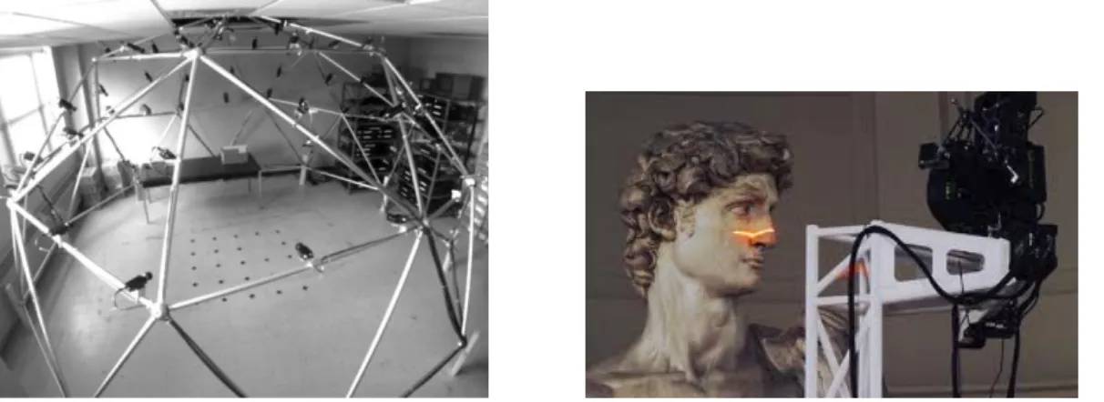
Sensors apprehend or digitize the surroundings around us. Of course, as for displays, the innovation started in specialized environment. For example, the 3D Dome was developed in Carnegie Melon University in 1995 for creating what they call virtualized reality sequences, that is, 3D + t data digitizing a real scene (Figure 1.4, left). The Digital MichaelAngelo project happened during the 1998-99 scholar year (Figure1.4, right); digitizing museum pieces has since spread. New 3D applications are developing very fast. Everyone can for example create its own 3D avatar from, portraying your own head (see Figure 1.5, left). The movie industry has been a big consumer for new sensor technologies. The production company Pixar laid a small renaissance of the animated feature film (with nearly 15 movies since Toy Story in 1995, the first computer generated feature film). Nowadays its renderer PR Renderman5 is the leading commercial renderer for Hollywood productions, and CGI animated movies (with the competing studio Dreamworks) are a mainstay of the cinematographic landscape. Prominent Hollywood productions also consolidated mixing virtual and real imagery as an integral part of modern enternainment artpieces (the special effect company ILM6contributed to Jurassik Park, the Star Wars saga, Men in Black series, Weta Digital contributed to the Lord of the Ring saga, Avatar). These productions require new ways of creating and managing 3D assets. To note, this trend was also made possible by advances in Computer Vision, which allowed such things as tracking the location of the camera in real footage (making a realistic integration with rendered image easier), acquiring the lighting environment of the scene and more recently tracking the articulated motions of real actors to replace them by virtual avatars. Besides, new types of cameras are offering to create 3D content: the first time-of-flight camera for civil applications Z-cam came out in 2000, as the semiconductor processes became fast enough for such devices http://en. wikipedia.org/wiki/Time-of-flight_camera#cite_note-ZCam_history-2. Today, the price of time of flight camera’s make them usable for private use. In 2009, Nintendo launched the Wii console, able to detect 3D motion and in 2010 Microsoft launched the Kinect. The Kinect, which use and price is meant for regular private consumers, has also been used for different applications.

4

For a example, seehttp://madebyevan.com/webgl-path-tracing/

5

http://renderman.pixar.com

6

(14)

1.1. Global context: the use of 3D models today 7

For example, Oikonomidis et al. [Oikonomidis 2011] use it for hand motion tracking, and Changa et al. and Chopping et al.[Changa 2011,Choppin 2012] propose to benefit from a Kinect sensor to guide disabled young adults (Figure 1.5, right). The evolution of sensors, and the fact that they are affordable, broadens the average consumer capability of capturing the surrounding real 3D world. However, we need to point out that our interaction with screens has also changed a lot in the last 10 years. Tactile screens offer new ways of interact. Although touch-screens existed for a long time: a short article appear as early as 1965 [Johnson 1965]), the first touch screen phone, the IBM simon, appeared in 1993. Nowadays, touch screens are everywhere; small kids’ ability to play on tactile devices is a witness to how intuitive touch based interactions are.

Figure 1.4: Acquisition of 3D or 3D+t content in specialized environments: on the left, the Dome from CMU (source: http://www.cs.cmu.edu/~virtualized-reality/page_History. html); on the right, scanning of Michelangelo David’s head (source: graphics.stanford.edu/ projects/mich/)

To wrap up our horizon tour on new devices, we have to mention another important tool (Figure

1.6). The first 3D printer has been developed by C. Chuck Hull 7. Early efforts at University of Bath by Adrian Bowyer and later developments made by the RepRap community8 to build a self-replicating 3d printer using patent-free technologies recently raised the industry and public awareness toward 3D printing technologies. 3D printing (which builds a solid object by layering microscopic slices of material, such as plastic, concrete or metal) has now been successfully used as an industrial design tool for rapid prototyping, in stop-motion animation for figurine making (e.g. in the movie ParaNorman9_{), in NASA for rocket engine parts and also for food} to be printed in space 10. The joint emergence of the maker movement, the hobbyist market and crowd-funding platforms lead to a rapid explosion of 3D printing products since the middle of the 2000. Many companies are now offering 3D printers targeted to the consumer market at increasingly affordable prices. Since the beginning of the century, the price of 3D printers have dropped significantly and they are common place. This technology widen the range of use of 3D modeling solutions, 3D assets sharing and manipulation. 3D printers have been labeled disruptive technologies11, that is, supposed to significantly make a difference.

7 http://www.pcmag.com/slideshow_viewer/0,3253,l=293816&a=289174&po=1,00.asp 8 reprap.org 9 http://www.wired.com/design/2012/07/paranorman-3d-printing/ 10 http://www.space.com/22568-3d-printed-rocket-engine-test-video.html 11

(15)

Figure 1.5: New common place application based on 3D sensors: on the left, the software EasyTwin c from digiteyezer allows to acquire and print (source: http:// www.digiteyezer.com); on the right, using the Microsoft’s Kinect as Navigation Aids for Visually Impaired [Choppin 2012] (photo from http://www.ubergizmo.com/2011/03/ visually-impared-kinect/)

Figure 1.6: 3D printing: The ultimaker 3D printer (left), and some printed (right). Figure 1.5

(left) also shows some printed figurines.

To sum up, 3D has become a really hot topic, as claimed in the call for paper in the Hot 3D conference12. The 3D community is obviously facing new challenges: providing new tools for creating 3D models, manipulating them (comparing, editing) and being able to share 3D content.

machines.

12

(16)

1.2. Different representations for 3D models 9

1.2 Different representations for 3D models

We have seen in the previous paragraph the general context, and some new, common place technologies and applications for which 3D models are required. We now review the different classical representations available for modeling 3D objects and their advantages and drawbacks. To model 3D objects it may seem natural to use volumetric data. Volumetric model-ing includes particle representations [Sims 1990] which is particularly adapted for fuzzy or fluid objects (usually in motion) like smoke or water. Other solid volumetric model are 3D meshes that are adapted for volumetric finite element computation or 3D visualization [Pain 2001,Gumhold 1999, Freitag 2002]. However, since the appearance of 3D object mainly depends on its exterior, a representation of the surface of the object, called boundary repre-sentation, is used in most applications. In our work, we only use surfaces for modeling 3D objects. As mentioned in the previous paragraph, parametric surface models are the most commonly used in CAD/CAM software [Farin 2002a]. NURBS [Piegl 1997] has become a standard for the parametric design software, and is now used by most software today, like CATIA from Dassault System13 or Creo from PTC (Parametric Corporation Technologies)14. These parametric surface models are either piecewise polynomial, or piecewise rational tensor product surfaces. They are also called free-form surfaces and are intuitively controlled by a set of control points and are generally smooth surfaces. Their smoothness is controlled by the knot vector and the degree of the underlying polynomials even though in practice degree 3 or 5 polynomials are used in most cases. Formally, a NURBS surface patch is a piecewise rational map, or more exactly the mapping of a 2D domain into 3D. The parametric representation offers the advantage to be able to easily generate points on the surface by simply considering the image of points in the domain. Moreover, information about the derivatives of arbitrary order is easy to compute (up to the continuity for a parameter value corresponding to a knot). The correspondence between the mathematical properties of the function/mapping and the surface depends on the parameterization (e.g. [Goldman 2002]). One way to keep a good correspondence, is to ensure that the parameterization is as regular as possible; for that, if the knot vector is regular, the control point should be regularly spaced [Farin 2002a,Tauber 2004] or the parametrization may be adapted considering arc length, or centripetal parametrization [Foley 1987]. Alternatively, geometric continuity may be used [Barsky 1984, Peters 2001]. In general, parametric models are used in applications where the quality and accuracy of the surface is important, both in terms of measure on the model and but also in terms of smoothness. Mesh models consist of a discrete set of vertices (the geometry), and a topology (a graph) defining the faces and edges of the surface. The minimum property required for a mesh properly model a surface is to be manifold (that is at every interior point locally homeomorphic to a disk) . Meshes are from far the most commonly used models, since they can be derived from a set of sample of points on the surface. Any arbitrary mesh can be easily triangulated (each face has three vertices). Triangulations are the only models to be natively rendered by graphic cards. Scanline rasterization algorithms for triangular facets are well understood and were implemented by the early dedicated hardware components, which further cemented the triangle mesh as the canonical surface representation. Unlike parametric surfaces, meshes are only continuous surfaces, with discontinuities of order 1 on the edges. Meshes are therefore used in

13

http://www.3ds.com/fr/products-services/catia/

14

(17)

applications where the rendering speed in the most relevant factor, and accuracy and smoothness is less important. However, a lot of papers have proposed techniques to evaluate approximate derivative information on a mesh, e.g. [Rusinkiewicz 2004, Morvan 2008]. Moreover, from the visualization point of view, rendering algorithms like Gouraud (or Phong) shading consider a set of continuous derivative of the mesh surface which smooths the appearance of the mesh. Modern rendering techniques such as normal mapping further decouple the 1st order derivative information (which can be made very detailed at a relatively low cost) from the geometrical information, making even low density meshes visually pleasant. One can also consider fine enough meshes so that the projection of a triangle on a display does not exceed a small number of pixels. Subdivision surfaces (e.g. [Warren 2001]) offer refinement operators on a mesh, so that a mesh can be refined to an arbitrary resolution and converges to a smooth surface. When the mesh is regular (triangulation where each vertex has valence six, or a quad mesh where each vertex has valence four) and for classical subdivision schemes (like Loop [Loop 1987] or Catmull-Clark [Catmull 1978]) or well-chosen schemes [Sabin 2010, Barthe 2011], the subdivision process actually converges to a parametric surface, namely a Box-spline. In the case of irregular vertices, particular rules are required, and an analysis of the behavior of the subdivision is done to study the smoothness of the resulting surface [Dyn 2002, Peters 2008] . Subdivision surfaces offer a good compromise between mesh and parametric representations. They naturally provide a multiresolution setting, and allow to easily work with surfaces of arbitrary topology. They have been used in the movie industry for more than 15 years now, and have also make their ways into CAD software. Recently, Pixar has released its modeling package into open source 15.

Another discrete representation for 3D models is the point-based representation. Points based models are a set of vertices on the surface. As mentioned in the previous section, point-based models have been around since 1985 [Levoy 1985] but got a growing attention since the years 2000 (e.g. [Pauly 2002, Gross 2011] as they could then benefit from programmable GPU to be rendered in real time [Guennebaud 2003]. Point based model can be presented intuitively in two ways. First, we may say that if a mesh is refined enough so that the projection of its faces on the screen just covers a couple pixels, then the topology information may be spared, and only the vertices can be kept. Neighboring vertices of a given vertex may be retrieved if necessary, simply by checking nearby vertices (for more details see [Pauly 2003a]). A second way is to consider point set surfaces as the generalization of meshes where one has reduced the continuity of the surface. Instead of having a C0 continuity surface, we now have a C−1 surface. In point set surfaces, the vertices are usually attached a radius, and a normal. Point based models are the raw data output by range 3D scanners, which make them ideal for early visualization applications, or for merging many scans into a single representation. Moreover, the lack of topology may also be an advantage for representing object with particularly complicated topology, like a tree [Guennebaud 2004], or for keeping independent geometric data, for example for streaming [Mondet 2007]. Most of the time, point based models are stored in a space partitioning data structure (like octree, or K-d trees), to ease the access to neighbors.

Another classical representation is based on implicit surfaces [Bloomenthal 1997]. Implicit surfaces are defined as the iso-surface of a potential function defined in R3. These surfaces are particularly interesting since they combine a volume and a surface representation. However,

15

(18)

1.2. Different representations for 3D models 11

their main drawback is that sampling points on the surface is a difficult task. A triangulation may be recovered after dicing the volume into a voxel grid and running a so-called marching cube algorithm. Thus, a classical rendering through a regular graphic pipeline is neither easy, nor efficient. As an alternative, rendering based on ray tracing is adapted for implicit representations (but not real time –yet).

Finally, imaged based representations (IBR, for Image Based Rendering) have been proposed mainly by the rendering community. Many representations and techniques were invented for image-based rendering (IBR), for example, the Lumigraph [Gortler 1996] and the light field [Levoy 1996], mosaics and panoramas (e.g. [Shum 2002,Peleg 1997,McMillan 1995]), and texture maps (e.g. [Debevec 1998, Buehler 2001]). A detailed survey is conducted by Zhang [Zhang 2004]. They use a set of images, possibly associated with depth maps or disparity to represent geometry and texture. Some approaches have considered multiresolution or multi-layered approaches [Shade 1998, Woodford 2005]. When the represented geometry corresponds to a single object, its image representation is called impostor. A detailed survey on this subject is presented by Jeschke and Wimmer [Jeschke 2005]. Schaufler [Schaufler 1998] also proposed layered impostors. In some work, impostors can also be textured depth mesh (TDM), as for [Aliaga 1999].

We have reviewed the classical 3D representations, and pointed out their advantages or drawbacks and applications for which they are preferred. In the work presented here, dif-ferent 3D models have been used, in order to benefit from their properties. Parametric models and parametric surfaces are used in two different settings: Chapters 2 and 3. In Chapter 2 about creating 3D models, parametric surfaces are used for shape from shading [Courteille 2006a, Courteille 2006b]. The choice of the underlying parametric reconstructed model not only insures the reconstruction of a smooth surface, but it also reduces the number of unknowns, which is necessary for the computability of the solution. In Chapter3, the model is the starting point, as we are interested in identifying parts of a classical CAD model that are sim-ilar up to an isometry [Dang 2012,Dang 2013]. Moreover, the parametric representation eases the computation of characteristics of a sample point on the surface, which is an advantage. We have used simple mesh models with textures in Chapter3when extracting semantic information from user interactions [Nghiem 2012,Nghiem 2013]. We choose these models for their popularity, since they are the most likely to appear on e-commerce applications. Meshes are also the most popular representation for 3D objects in virtual environments, so, in Chapter4, we have consid-ered meshes for the transmission of 3D models [Cheng 2007,Cheng 2011,Zhao 2013]. We use for that the classical progressive mesh representation from Hoppe [Hoppe 1996]. In this document, point set surfaces are used in Chapter3in a tracking algorithm [Dehais 2006,Dehais 2010]. As we assume that a 3D model of the object is known, it is actually not necessary to define the topology of the set of point of the object. Having just a set of point saves the definition of the topology, and allows to directly consider the scan of an object as an input to our algorithm. We actually also have used point-based model in the context of 3D streaming (Chapter4), but this work is not presented here for keeping the material reasonably concise (more details can be found in [Mondet 2007]). We also use in this document, both in Chapter 2 and Chapter 3, a curve based representation for representing plants, and in particular plant branching structures. In Chapter2, we create a realistic model of a plant from biological knowledge of its species and a single image [Guénard 2009, Guénard 2010, Guénard 2011, Guénard 2012, Guénard 2013b]. In Chapter 4 we propose a compact and progressive representation for trees branching

(19)

sys-tems and use it for efficiently transmitting plants models over a potentially lossy network [Mondet 2007, Mondet 2008,Mondet 2009b, Doran 2009]. In section 4.6 , we proposed to use image based representation to ease access to NVE (Networked Virtual Environments) for light clients. We consider IBR first to limit the size of the data to be sent, and also to simplify the rendering task for the light client [Zhu 2011].

Note, that we do not consider stereo vision, although these representation are already quite advanced in the context of democratizing 3D, e.g. 3D displays are mostly based on stereoscopic images. Our work focuses on actual 3D models that do not depend on the viewpoint. However, in our context the interactions between the three dimensional world and their images (or sequence of images) in 2D are important, as we highlight in the next section.

1.3 3D and 2D

Considering the rendered image of a given 3D model is necessary since we apprehend the 3D constructed models mostly through flat 2D screens. However, handling a 3D model is very different than working with 2D content. A 3D object appears on the screen as a 2D image, but their 3D nature is still present. First, viewing parameters may be chosen and changed: the viewpoint, of course, is free and allows navigation around the 3D model. Also, lighting parameters, and even the color of the model may be changed. So, interacting with a 3D model is much richer than just viewing a static image of this model. In Chapter3, we make a first step towards simplifying user interactions with 3D content, by linking viewing parameters to simpler information: a text description. In Chapter 4, we propose an alternative to previewing a 3D model in a 2D video, by rather displaying well chosen views of the 3D content while downloading the model. In both cases, a simpler representation (text or image sequence) is used to restrict the access to 3D, in the first setting to limit the degrees of freedom in navigation, in the second to leave some time for downloading the model while adapting the transmission to the ongoing interaction (simulation of a video).

Moreover, images and videos have already made their ways in our daily life (we use in the following the term 2D content to denote both images and videos). Since numerical cameras, and video cameras are now included in every mobile phone, the diffusion of 2D data has been very demanding on solutions for storing analyzing and sharing this content (100 hours of video are uploaded to YouTube every minute16). These 2D content, images or videos representing the real 3D world, offer almost unlimited resources for apprehending 3D models. We indeed start from images for creating 3D content in two different applications of Chapter 2. Moreover, in Chapter 3, the proposed tracking algorithm finds the position of a 3D model within a video. Finally, in Chapter 4, we consider peer-assisted-rendering : in a popular NVEs where numerous clients evolve, users with limited resources request pre-rendered 3D objects to users with spare rendering cycles in order to simplify their own rendering. These interactions between 2D and 3D content have led to convergence between different research communities. The Computer Vision and Computer Graphics communities are getting closer; topics like stereovision, and 3D reconstruction are really shared between these communities. Moreover, communities like the computational geometry, signal processing, and Multimedia community are also getting involved in 3D modeling. For the signal processing community, they have been applying their methods to 3D data: for example, much work on

16

(20)

1.3. 3D and 2D 13

compressing 3D data has been done by signal processing researchers (see Chapter 4, section

4.3.3). Similarly, 3D content is a new media to store, edit and distribute for the multimedia community. As some multimedia technique may apply the same way to all media, some specific approach may need to be deploy for 3D content (see Chapter4, section4.2.1).

A final note on 2D content: this document will not mentioned some work done on 2D images (compression [Delaunay 2007a, Delaunay 2007b, Delaunay 2008a, Delaunay 2008b,

Delaunay 2010] and 2D+t image sequences (tracking [Tauber 2004,Parisot 2004,Parisot 2005a,

Parisot 2005b]) for coherence reasons, as this document focuses on 3D content.

Organization of the manuscript

To conclude on the concerns raised in 2001 in the SIAM/GD meeting: we have seen that a brand new challenge for the geometric modeling community has emerged: democratizing the use of 3D content. As discussed, some collaborations with different research communities will certainly be relevant. 3D content will still be used by CAD companies, and the entertainment industry, in both context requiring new models, tools, methods and developing new dedicated material. However, 3D content will also be more present as multimedia content in our daily life. To that end, we need to develop new tools for creating, manipulating and sharing 3D content. In Chapter2 will present two dedicated methods for creating 3D models from a single image. For the use of 3D models, new, intuitive and efficient tools will be necessary. Chapter3present three contributions for manipulating 3D content. The first one proposes an original tracking algorithm to follow a 3D object whose model is known through a video sequence. The second one analyzes 3D models for identifying partial similarities in parametric models. The third contribution simplifies the interactions of regular users with an online 3D model, for applications e.g. in the context of e-commerce. Finally, Chapter 4addresses the problem and the specificity of the transmission of 3D content. We consider, and develop, progressive models for plants, and derive streaming strategies considering possible packet losses.

(21)

(22)

Chapter 2

Creation of 3D models

Contents

2.1 Introduction . . . 15

2.2 Modeling plants from one image . . . 17

2.2.1 Previous work. . . 17

2.2.2 Extracting a 2D skeleton . . . 20

2.2.3 Generating a 3D plant model . . . 27

2.2.4 Model selection: a Bayesian approach . . . 29

2.2.5 Results . . . 30

2.2.6 Conclusions, limitations and perspectives . . . 34

2.3 Generating 3D from one image: Spline from Shading. . . 36

2.4 Conclusion, limitations and perspectives . . . 39

2.1 Introduction

The first step for an extended use of 3D models is to generate 3D content. There are two ways to model 3D objects: Computer Aided Design (CAD) or digitizing an existing model. The first way is to generate virtual objects. This part is concerned with synthesis. These virtual object may be intended to be produced, for example, when creating a new car model using a CAD system; but, these object may also be intended for staying virtual, like our favorite figures in animation movies, monsters in video games, or explanations added to a tool in the setting of augmented reality. In both setting, the 3D object is designed using a software, depending on the considered application; some examples of modeling software are Blender (an open Source software), Maya or 3ds max (from Autodesk, the first one rather for the film industry, to second one for the game industry), Rhino (from Robert McNeel & Associates), or CATIA (from Dassault System). For using a CAD software however, a particular training is necessary. Moreover, the process of creating a 3D model from scratch is quite time consuming, and requires not only good technical skills from the designer, but also a good domain knowledge, or artistic skills.

The second way is to model real existing objects. For that, 3D sensors may be used. We already have talked about digitizing museum pieces with a scanning device e.g. [Levoy 2000]. In medicine, 3D models may also be reconstructed from 2D slices or volumetric sensors, like VCT (Volumetric Computed Tomography). These methods are classified as active reconstruction methods, since they interact with the object. On the opposite, image based reconstruction methods are also called passive methods.

(23)

In this Chapter, we present the results of two passive methods for generating 3D objects. In both cases, we assume some knowledge on the final object, in particular by restricting the 3D model. First, we briefly review general reconstruction from multiple images.

The work presented in this chapter has been developed in the context of the doctoral work of Jérôme Guénard (plant modeling), and Frédéric Courteille (Shape from Shading). For the first part (section2.2), more details can be found in Jérôme Guénard’s dissertation [Guénard 2013a], co-advised with Pierre Gurdjos and Vincent Charvillat. The plant modeling work was done in collaboration with Frédéric Boudon from CIRAD. The contributions have been published in [Guénard 2010,Guénard 2011,Guénard 2012,Guénard 2013b]. The second part was developed in the context of Frédéric Courteille’s Ph.D.; I collaborated with him and his advisor Jean-Denis Durou for a common publication [Courteille 2006a].

3D reconstruction from images

Intrinsically, 3D reconstruction from a set of images is a difficult problem. A realistic 3D reconstruction of a small 3D object can be generated from a set of well chosen images, taken in good conditions, with careful calibration. Seitz et al. [Seitz 2006] propose benchmarks and comparison of different reconstruction algorithm are given on the corresponding website http: //vision.middlebury.edu/mview/eval/ (Figure 2.1). The minimal set of images considered contains 16 images. Images with shadows have been removed from the data set and radial distortion removed. The parameters of the camera are given for each image. This benchmark

Figure 2.1: The two 3D models proposed as benchmarks for 3D reconstruction algorithm [Seitz 2006].

shows that 3D reconstruction can be achieved in very controlled environment.

Other work achieved a good 3D reconstruction from images taken in arbitrary conditions: Goe-sele et al. [Goesele 2007] use online photos of famous monuments to reconstruct a 3D model. The number of input images is very large (several hundred images). This work applies to famous buildings, for which many images are available.

A different approach reduces the degrees of freedom in the reconstruction by introducing domain knowledge on the model. For example, Bey et al. [Bey 2012] recover some 3D objects in an industrial environment (from 3D point clouds) assuming the 3D object belong to a set of

(24)

2.2. Modeling plants from one image 17

predefined shapes (cylinders and spheres) since they know they are in an industrial setting where the 3D object are mostly pipes.

In this chapter, we use a similar approach. First, in the context of plant modeling, we use L-systems, a classical generating method. However, our reconstruction is based on the shape given by an image of the plant. Using the image insures the realism of the model, avoiding the fractal-like natural regularity of plants generated by L-systems. Moreover, the particularity of plants is to have a very complex topology, and also to be highly self similar. Correspondences are hard to find, and there is not much depth coherence. For these reasons, we consider a single image. Then, we show results on reconstruction from a single image in a different context. In the following, we first review the classical models for plants and previous work on modeling plants from images.

2.2 Modeling plants from one image

2.2.1 Previous work

2.2.1.1 Plant modeling

Plants are important and common objects of our world. Just as in the real world, plants help create pleasant and realistic virtual environments, especially those involving natural scene. Realistic modeling of plants are crucial applications such as virtual outdoor scenes like virtual botanical gardens, where users are expected to inspect a plant closely and possibly interact with plants. Previous work has focused on how to accurately model a plant, e.g. [Remolar 2002,

Bloomenthal 1985, Prusinkiewicz 1990,Prusinkiewicz 2001]. Realistic and detailed plant mesh models can require up to hundreds of thousands of polygons. Remolar et al. [Remolar 2002] estimated that a plant generated by XFrog1, a well known plant modeling platform, can consists of 50,000 polygons to represent the branches. The plants can have 20,000 or more leaves, which themselves consists of polygons. Neubert et al. [Neubert 2007] reported the plant models that they used consists of up to 555,000 polygons. These numbers are for a single plant.

As plants are, by nature, very self similar, associating redundant parts within a plant model allows to simplify the model, and to a more compact numerical representation. For example, the leaves of a given tree maybe represented by a small number of models, instantiated several times. The pioneering work of Lindenmayer [Lindenmayer 1968] proposed to formalize the re-dundancy within plants by modeling plants using L-systems. The idea is to model a plant as a formal language, thus following a limited, simple generating rules. This modeling technique has since became a standard for plant modeling [Prusinkiewicz 1990, Deussen 2005, Weber 1995]. However, a simple deterministic application of the generating rules of a L-system leads to very self similar plants, similar to fractals ??. But plants are also characterized by their irregulari-ties. Thus to create realistic plants, irregularities are necessary but need to be coded, leading to a compromise between the compactness and the realism of the model [Boudon 2006] (see Figure 2.3). Prusinkiewicz has proposed to use non deterministic rules in order to generate irregular plants [Prusinkiewicz 1990]. Some authors derive the probabilistic laws from botanical studies [de Reffye 1988, Chaubert-Pereira 2010] to generate a random, irregular instance of a plant. Other approaches consider physical constraints. For example, both Palubicki et al. and Runions et al. grow a plant within a given volume, where branches compete for filling the space [Palubicki 2009,Runions 2007].

1

(25)

Figure 2.2: Generating plants like fractal, using simple deterministic L-systems.

Figure 2.3: Three instances of plants modeled with the L-py softwarehttp://openalea.gforge. inria.fr/wiki/doku.php?id=packages:vplants:lpy:main. From left to rigth, as irregulari-ties appears, the plant becomes more realistic.

(26)

These different approaches propose to generate models of plants using generative models corre-sponding to a species following some botanical or physical rules, and create a particular, irregular and realistic instance using external constraints. An alternative way to model a particular in-stance, is to model an existing plant. Plant modeling from one or several image proposes to model a particular instance of plants. In the next section, we review different approaches for modeling plants from images.

2.2.1.2 Modeling plants from images

Procedural method based on L-systems can model the growth of a plants, and follow its evolution. The methods based on images only give a model of a plant at a particular point in time, namely, when the image has been taken.

Some methods are based on 3D reconstruction of a set of points. For that, and because plants are very self similar, 2D point correspondences is challenging. Quan and al. first proposed to model simple plants from a set of images [Quan 2006]. The set of images need to be sufficiently dense for the 3D points to be extracted with a structure from motion algorithm. The plant consists in stem and leaves, so leaves are positioned using the reconstructed 3D points, and corresponding deduced. Tan et al. [Tan 2007] adapted the preceding method to tree modeling. Similarly, a set of 3D points is extracted from structure from motion. The 3D reconstruction is used two ways: first, the point set defines a volume, in which branches are generated. Second, visible branches are reconstructed. The structure of the branching system is extrapolated from the visible branches structure.

Other methods extract a volume from the silhouette of a tree in several images. In that setting, no 2D point correspondences is needed, and there may be fewer images. Both Reche-Martinez et al. [Reche-Martinez 2004] and Neubert et al. [Neubert 2007] extract a volume where they attach attributes. In the first paper, they generate real time volume representation of trees to be inserted in virtual environments. Neubert et al. generate a real 3D model of the tree. The branching system grows interpolating a set of particles withing the volume.

Finally, in a more recent work, Li et al. consider a video as the input, and generate a dynamic 3D model of the tree. They also derive dynamic properties of the 3D model to animate it through the wind, and also proposed to generate similar but different trees in order to create forest. Similar to Wang et al. [Wang 2006] analyze a set of images of trees of the same species and from this analysis to generate realistic model of trees of the same species.

In these approaches, a dense set or a sequence of images is required (point correspondences may be identified only of the set of images is dense enough). We now look at methods were a single image suffices.

2.2.1.3 Modeling plants from a single image

First, let us make a detour to approaches based on sketching; they are related to methods using a single image since they usually consider also only one viewpoint. Okabe et al. propose to sketch the shape of the branching system in 2D and use it to infer their position in 3D [Okabe 2005]. [Runions 2007], [Wither 2009] and [Talton 2011] ask the user to sketch in 2D the volume of the foliage. Runions et al. iteratively grow the branching systems to progressively fill the volume, whereas Wither et al. proposes an interactive multiresolution approach to progressively define the shape of the branches inside the volume. Talton et al. use a formal grammar (like L-systems) that they control to fill up the desired volume. Some other approaches mix image and sketching,

(27)

asking the user to draw on an image of the plant. For example, Liu et al. [Liu 2010] use the annotated image to reconstruct 3D points, and define a 3D embedding volume.

The following method are based on a single image, but as some require user interaction, they are indeed quite similar to approaches involving sketching. Tan at al. [Tan 2008] propose to reconstruct trees from a single image, but requires user interaction to outline the foliage volume and draw the visible branches. Using the visible branches shapes as pattern, a branching system is generated inside the volume 2.4. The method proposed by Zeng et al. [Zeng 2006] is using

Figure 2.4: The pipeline proposed by Tan et al. for reconstructing a tree from a single image. User interaction is required to segment the foliage and mark the visible branches (images from [Tan 2008]).

images of branching systems, and reconstruct a tree without the leaves first in 2D, and then embeds it in 3D space while defining a volume for the leaves.

The existing methods require some user interactions (method based on sketching, [Tan 2008]) or/and visible branches ([Tan 2008,Zeng 2006]). In the next section, we propose a fully auto-matic approach for reconstructing plants from a single image. We start with plants of a given species, here wines. We then generalize our methods to trees: for that, we need to get a plant in 3D and work with a multiresolution scheme. Visible branches are not necessary, as we assume a prior knowledge on the plant species, and use some botanical knowledge for creating the branch model. Thus, the generated model is biologically sound, and also realistic since it fits a existing instance (on the image).

2.2.2 Extracting a 2D skeleton

We have first worked in the context of vine modeling as explained in the next paragraph: our goal is to develop a fully automatic method, unlike the methods proposed in the related work. Moreover, we can not rely on the assumption of having visible branches (see for example Figure

2.5).

2.2.2.1 The context

This work was done in the context of the projetc VINNEO which goal was to propose innovating techniques in order to improve the quality of the local wine2. Our participation aimed at characterizing vine properties based on images. Differences between different vine plots, or within a vine plot, should be identify for clustering the grapes into different products (wine). For example, an important factor is the SECV (Surface Exposée du Courvert Végétal in french, Exposed surface of the foliage). It corresponds to the total surface of all the leaves of a vine. Studies have shown, that to properly mature a kilogram of grapes, the vine needs from 0.5 to 2 square meters of SECV depending on the species, weather conditions or the type of wine

2_{http://www.inp-toulouse.fr/fr/partenaires/innover-avec-l-inp-toulouse/}

(28)

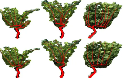
produced. The ratio between leaves and fruits is calculated by dividing the SECV by the plot performance. It is therefore useful for winemakers to estimate the SECV on different plots in order to define the number of clusters/products to consider on a given vine plot. Today, this index is just estimated by eye, the winemaker simply looking at the wines. We thus proposed to embed a camera on the tractor in order to automatically extract the SECV from the images. As an intermediate step, we reconstruct a 3D vine plant for these images. An automatic method segments the foliage, based on the assumption that the camera motion is linear and parallel to the wines (more details are given in [Guénard 2013a]). Then, the images are rectified, to get a fronto parallel view of the plants. The resulting image is therefore of limited quality.

So, the method we developed is adapted to this context: we assume that we know the species of the plant, wines, and benefit from the fact that the vines grown in a plane (because of the trellising). The fist step of the proposed method consists in extracting a branching structure from the foliage segmentation in a 2D image. The goal of this method is to extract a possible skeleton, from which a plant is generated, and its projection is then compared to the original binary shape.

A proof of concept

First, we wanted to assess that it is indeed possible to estimate a skeleton from the binary shape of the foliage, with biological knowledge on the plant. We asked two wine experts3 to draw the structure of the branches on images of vines rectified in the plane where they grow – We assume that the entire structure of the plant is in the same plane as the branches are attached on parallel iron wires by the winemakers. The resulting drawings from the two wine experts are shown in Figure2.5. First, their knowledge on the plant growth and the human interaction (pruning and

Figure 2.5: Example skeletons estimated by two different wine experts on three different vine plants.

trellising), together with the visible foliage information allowed them to quite quickly and easily propose a skeleton for the plant, and, as a matter of fact to guess the type of pruning of the

3_{Eric Serrano, Regional Director of the French Institute of Vine and Wine southwest and wine and engineer}

(29)

mother branch –the branch attached directly to the trunk. Moreover, the experts found in all cases (15 plants) very similar mother branch shapes, a consistent number of branches (equal up to one or maximum two branches), and coherent branches shapes. So, together with their knowledge on the plant, the shape of the foliage projection provides them enough information to estimate a relatively stable branching structure.

Thus, our goal is to automatize the process of finding branching structures similar to the branches traced by experts. We are naturally interested in the skeletonization of a binary form and we sought to develop a method such that it is possible to take into account a prior knowledge related to biological constraints.

Skeleton extraction: related work

Skeleton curves are used in many applications in 2D and 3D. In particular, they may be used for giving a simple and intuitive representation of the object, and as such are useful for editing or animating objects. In our setting of plant modeling, the goal is to extract the curve structure, that is, its branching system. The most classical skeleton is the medial representation of a 2D shape and has multiple definition. Intuitively, the medial axis is the locus of points located in the middle of the shape; each point has a corresponding local thickness. Blum [Blum 1967] first defined the medial axis as the set of the centers of maximal balls. A ball is maximal if it is included in the shape, and is not contained in any other ball included in the shape (see Figure 2.6 left ). An alternative definition is to define the medial axis as the locus of the set of points having at least two closest points on the boundary (see Figure 2.6 middle). Amenta et al. [Amenta 1998] showed that for C1 boundaries, the sphere centered on the medial axis and passing through the two closest point is tangent to the boundary. Finally, assuming a fire propagates from the boundary to the interior of the shape, the medial axis is also defined as the location where two or more burning fronts meet (see Figure2.6right ). The main drawback

Figure 2.6: Three different definitions of the medial axis: centers of maximal balls (left ), points having at least two closest neighbors on the boundary (middle), and shock graph of a grass-fire evolution from the boundary (right ) (images from [Tagliasacchi 2012]).

of medial axis skeletons is their lack of robustness. Many authors have proposed approaches to prune the medial axis in order to keep important or stable parts (see [Attali 2009] for a survey). In [Shlyakhter 2001], the authors propose to use the medial axis to generate a branching structure of a tree. When the leaves are added to this branching structure, the tree with foliage has a satisfying shape. However, the branching structure itself is not realistic: it look very different than a natural branching system, in particular since branches are not growing up but in any

(30)

direction. Indeed, many properties of the medial axis are useless for our setting. For example, the medial axis preserve the homotopy type of the shape. In the case of a binary shape modeling the projection of the foliage, holes may appear but do not necessarily require an additional branch to be generated. Also, a branch/skeleton does not need to be centered. For that reason, we propose to adapt the skeleton extraction method of Cornea [Cornea 2005] (a comparison of classical methods for skeleton extraction and their respective properties is given by Cornea et al. [Cornea 2007]). Cornea et al.’s method produces a skeleton which is not necessarily homotopic to the shape, neither centered. However, the skeleton is connected, robust (stable to small changes), and smooth. This skeleton will define the branches of the tree.

2.2.2.2 The proposed method

Cornea’s original method

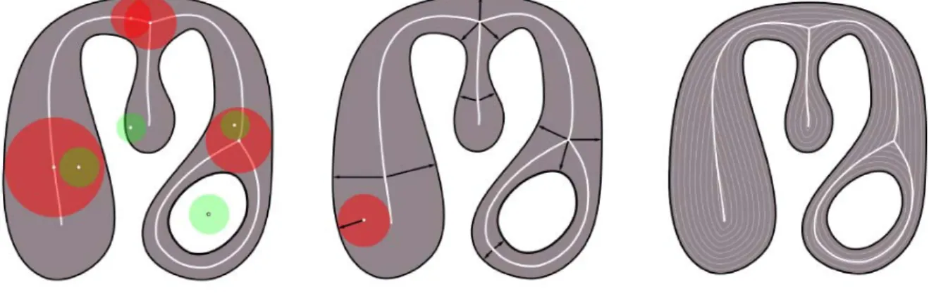
We start with a discrete binary shape corresponding to the segmented foliage projection, that is, a connected set of pixels. We consider 8-connectivity, that is, any pixel has eight direct neighbors. Cornea’s original method [Cornea 2005] takes two steps (Figure 2.7):

• First, we define a vector field on the shape. Each pixel p_iof the binary shape B is associated a vector pi, computed as the weighted average of the pixels mi on the boundary Ω:

− → fi = X mj∈Ω 1 ||−−−→mjpi||2 −−−→ mjpi ||−−−→mjpi|| . (2.1)

• Second, the inner pixels pi such that piis closed to zero are defined as critical points. The

skeleton consists in the paths from the critical points following iteratively the vector field.

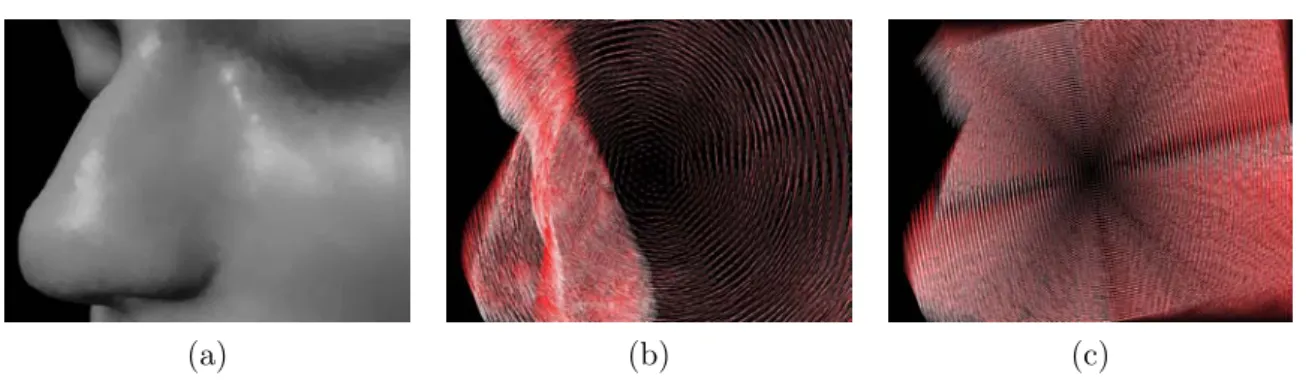
(a)

(b)

(c)

Figure 2.7: Cornea’s original algorithm on a binary shape corresponding to a vine foliage (a). The boundary Ω appears in red. (b) The vector field computed on the binary shape by equation

2.1), and the corresponding critical points in blue. (c) The extracted skeleton, in green.

Adapting the skeletonization for a branching system

To extract a skeleton of the binary shape modeling a branching structure, we need to inject some domain/botanical knowledge. First, we want to enforce some anisotropy, since branches grow up. Second, we want to have more than one branch in large area. Our idea is to artificially create contour points within the binary shape, in order to partition the skeleton, as illustrated in Figure2.8

We want to partition the segmented foliage in areas potentially covered by one branch. For that, we define some so called cuts in the binary shape. This segmentation is done following some botanical knowledge on the branches shape (like the angle with the trunk) and the shape of the foliage. As we aim to produce multiple models and select the best one, the parameters for the cuts are random variables.

(31)

Figure 2.8: The skeleton extracted from Cornea’s original method, using the red boundary (left). If we artificially partition the initial shape adding some boundary point, the skeleton will respect these boundary: our goal is to partition the shape in ordre to avoid vertically large areas.

Partitioning the binary shape

The cuts are defined iteratively, the starting points are chosen based on biological assumption on the plant species. For example, for monopodial plants, that is, plant whose branching system is organized around a central trunk, we give the interval between successive branches, as well as the angle between the branches. For vines, the number of branches, and therefore the number of cuts, is also defined as an input of the algorithm. For finding the ending point of the cut, a DCE (discrete curve evolution) algorithm [Latecki 1999] is applied on the boundary Ω of the plant in order to characterize and favor the inward angles of the shape as illustrated in Figure

2.9.

Figure 2.9: On the left, the foliage and its boundary Ω. In the middle, and right, the DCE curve with respectively 14 and 8 vertices. Vertices of inward angle ≤ π are shown in blue: they most likely indicate the limit between two branches regions.

Cuts are then chosen iteratively among DCE vertices, following a density of probability to favor inward angle. A filter avoids taking cuts too close to each others, or crossing. Each given cut is associated a probability which is the used as prior knowledge 2.2.4. More details can be found in [Guénard 2013a]. Figure2.10 shows two examples of cuts, one for vines and one for a monopodial plant.

Probability map on the binary shape

The cuts are not given directly to the skeletonisation algorithm; we first apply a horizontal smoothing (one dimensional Gaussian filtering) to avoid branches to follow too closely the shape of the cuts. Figure 2.11 shows an example of the probability map corresponding to the cuts of Figure 2.10. Then, we generalize Cornea’s vector field computation to take into account all

(32)

Figure 2.10: On the left, cuts for 5 branches on a vine. On the right, cuts for a monopodial plants (the cuts are cubic curves so a end point and a tangent is given on each side of the cut.

Figure 2.11: Probability map P corresponding to the cuts of Figure2.10left.

interior points with a non zero probability to be a contour point: − → fi = X mj∈Ω 1 ||−−−→mjpi||2 −−−→ mjpi ||−−−→mjpi|| + X pj∈B\Ω j6=i Pj ||−−→pjpi||2 −−→ pjpi ||−−→pjpi|| (2.2)

Figure2.12 shows the resulting vector field.

Figure 2.12: The vector field computed from the probabilty map on Figure2.11using equation

2.2.

The last step of Cornea’s algorithm is applied to define the skeleton, or set of attracting points that will be used to fit the branching system (Figure2.13) .

(33)

The branching system

We now need to fit a parametric model of the branching system with the attracting points describing the skeleton of the binary shape. The parametric model has been created in L-py [Boudon 2010] and each branch is modeled by a degree 3 Catmull-Rom curve [Catmull 1974] . The control points are computed in order to fit the parametric model and the attracting points using (in a least square sens). Figure 2.13 shows the resulting branching system for the vine. Note that the resulting skeleton branches give a realistic branch structure. Moreover, they not only fill the space in a way coherent with the boundary shape, but also avoid the holes in the binary shape.

Figure 2.13: The skeleton computed from the vector field2.12.

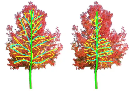
Hierarchical branching system

For more complicated plants, the partitioning is used iteratively, as illustrated by Figure2.14.

Figure 2.14: On the left, the first order branches –in cyan– (attached to the trunk –in green–) are computed using our approach. Then, on each cell (an area between cuts), the algorithm is applied recursively to find second order branches. On the right, second order branches appear in yellow.

(34)

2.2.3 Generating a 3D plant model

From the branching system in 2D, we now want to define a real plant in 3D. For that, we first need to infer a 3D plant from the 2D branching system extracted in the previous session. Then, branches are added a thickness and texture, and more importantly leaves are added to the model. Finally, we use a selection criteria measuring the posterior probability for choosing among several possible models.

2.2.3.1 A 3D skeleton

For the vines examples, the 2D skeleton is general enough since main branches are attached in a same plane. However, in general trees grow in 3D! We treat here the case of monopodial trees, and follow the work of [Zeng 2006] and [Okabe 2005].

First, we want to maintain the correspondence between the 2D binary shape and the 3D model, that is, we require that the projection of the 3D tree still fits the 2D segmented foliage. For that, we define a 3D volume in which the branches will grow: each horizontal segment of the 3D shape is associated a 3D horizontal circle. Together, these circles define a volume (Figure

2.15). In order to avoid the 3D volume to be biased in the direction of the foliage projection, the depth of the circle centers follows a Gaussian density centered on 0.

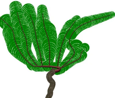
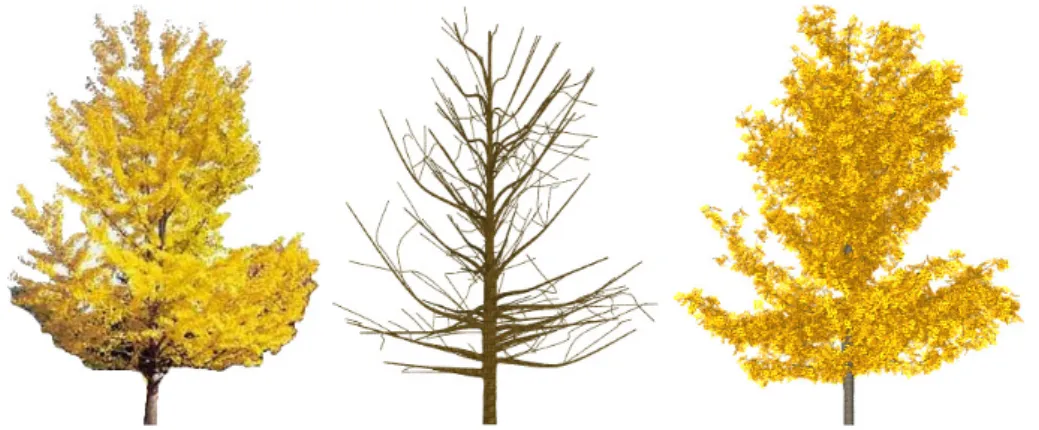
Figure 2.15: On the left, the original image of the liquidambar (sweetgum) with a segmentation of its foliage in 2D. On the right, the considered envelop for the foliage considered in 3D. Each branch that does not reach the foliage boundary Ω is turned so that it reaches the volume boundary. However, the branch could be going towards the front or the back. Following Okabe et al’s [Okabe 2005], the branches are spread as to maximize the angle between two branches from a top view. Also, branches need to be added to get a tree with a good density: several skeletons are computed and eroded to generate enough branches (Figure 2.16).

Figure2.17 shows an example of 3D skeleton extracted from our method. 2.2.3.2 Texture and leaves

The branching system is then represented with a thickness and texture. Textures from the tree species are used. The radius of the branch is a function of the distance of the branch to the trunk and the order of the branch. Parameters for the leaves are extracted on the 2D skeleton:

(35)

Figure 2.16: On the left, the skeleton after a small erosion. On the right, the skeleton after a larger erosion.

Figure 2.17: On the left, the input image for the liquidambar. In the middle, the complete skeleton seen from the same viewpoint. On the right, the same skeleton seen from another viewpoint.

• a leave radius (Figure2.18) is attached to each point of the branch, as the length of the segment on the line perpendicular to the tangent of the branch, and included in the cell of the branch (the cell is the area between cuts);

• a density factor corresponding to the percentage a foliage pixels in the cell is also attached to the branch.

On the generated models, the leave parameters are random variables following a Gaussian law whose mean is the computed value. Figure4.16illustrate the use of the leave radius and density influence.

(36)

Figure 2.18: On each branch, circles illustrating the computed leaves radius.

(a)

(b)

(c)

(d)

Figure 2.19: The same branching system with varying parameters for the leave radius rf and

density d_f: (a) r_f and d_f small (a), (b) r_f and d_f large, (c) r_f small and d_f large, and (d) r_f large and d_f small.

2.2.4 Model selection: a Bayesian approach

So far, we have proposed the construction of a model of a tree, following density functions depending on both knowledge of the species of the tree, and on the shape of the foliage. Some prior knowledge can also be added: in the case of vines, for example, we can give a probability for the shape of the main branch depending on the region where the vine grows. Also, we have observed the number of branches in the vineyards where we went: the average number of