O
pen
A
rchive
T
OULOUSE
A
rchive
O
uverte (
OATAO
)
OATAO is an open access repository that collects the work of Toulouse researchers and
makes it freely available over the web where possible.
This is an author-deposited version published in :
http://oatao.univ-toulouse.fr/
Eprints ID : 12220
To link to this article : DOI :
10.5194/hessd-11-7689-2014
URL :
http://dx.doi.org/10.5194/hessd-11-7689-2014
To cite this version :
Ferrant, Sylvain and Gascoin, Simon and Veloso, Amanda and
Salmon-Monviola, Jordy and Claverie, Martin and Rivalland,
Vincent and Demarez, Valerie and Dedieu, Gérard and Ceschia, Eric
and Probst, Jean-Luc and Durand, Patrick and Bustillo, Vincent
Agro-hydrology and multi temporal high resolution remote sensing:
toward an explicit spatial processes calibration.
(2014) Hydrology
and Earth System Sciences Discussions (HESSD), vol. 11 (n° 7). pp.
7689-7732. ISSN 1812-2108
Any correspondance concerning this service should be sent to the repository
administrator:
[email protected]
Agro-hydrology and multi-temporal high-resolution remote sensing:
toward an explicit spatial processes calibration
S. Ferrant1,2, S. Gascoin1,3, A. Veloso1,3, J. Salmon-Monviola4,5, M. Claverie6,7, V. Rivalland1,3, G. Dedieu1,2, V. Demarez1, E. Ceschia1, J.-L. Probst8,9, P. Durand4,5, and V. Bustillo1
1Université de Toulouse, UPS, Centre d’Etude Spatiale de la BIOsphère (CESBIO), 18 av. Edouard Belin, bpi 2801, 31401
Toulouse, Cedex 9, France
2Centre National d’Etudes Spatiales (CNES), CESBIO, Toulouse, France 3CNRS-CESBIO, Toulouse, France
4INRA – UMR1069 Sol Agro et hydrosystème Spatialisation (SAS), 35000 Rennes, France 5Agrocampus Ouest, UMR1069, SAS, 35000 Rennes, France
6Department of Geographical Sciences, University of Maryland, College Park, MD 20742, USA 7NASA-Goddard Space Flight Center, Greenbelt, MD 20771, USA
8Université de Toulouse, UPS, INPT, Laboratoire d’Ecologie Fonctionnelle et Environnement (EcoLab), ENSAT, Avenue de
l’Agrobiopole, BP 32607 Auzeville-Tolosane, 31326 Castanet-Tolosan Cedex, France
9CNRS, Ecolab, ENSAT, Avenue de l’Agrobiopole, Castanet, France
Correspondence to: S. Ferrant ([email protected])
Abstract. The growing availability of high-resolution
satellite image series offers new opportunities in agro-hydrological research and modeling. We investigated the possibilities offered for improving crop-growth dynamic simulation with the distributed agro-hydrological model: topography-based nitrogen transfer and transformation (TNT2). We used a leaf area index (LAI) map series de-rived from 105 Formosat-2 (F2) images covering the period 2006–2010. The TNT2 model (Beaujouan et al., 2002), cal-ibrated against discharge and in-stream nitrate fluxes for the period 1985–2001, was tested on the 2005–2010 data set (cli-mate, land use, agricultural practices, and discharge and ni-trate fluxes at the outlet). Data from the first year (2005) were used to initialize the hydrological model. A priori agricul-tural practices obtained from an extensive field survey, such as seeding date, crop cultivar, and amount of fertilizer, were used as input variables. Continuous values of LAI as a func-tion of cumulative daily temperature were obtained at the crop-field level by fitting a double logistic equation against discrete satellite-derived LAI. Model predictions of LAI dy-namics using the a priori input parameters displayed tempo-ral shifts from those observed LAI profiles that are irregularly
distributed in space (between field crops) and time (between years). By resetting the seeding date at the crop-field level, we have developed an optimization method designed to ef-ficiently minimize this temporal shift and better fit the crop growth against both the spatial observations and crop pro-duction. This optimization of simulated LAI has a negligible impact on water budgets at the catchment scale (1 mm yr−1 on average) but a noticeable impact on in-stream nitrogen fluxes (around 12 %), which is of interest when consider-ing nitrate stream contamination issues and the objectives of TNT2 modeling. This study demonstrates the potential con-tribution of the forthcoming high spatial and temporal reso-lution products from the Sentinel-2 satellite mission for im-proving agro-hydrological modeling by constraining the spa-tial representation of crop productivity.
1 Introduction
Agro-hydrological modeling was first developed and applied to study the qualitative and quantitative impacts of agricul-ture on water resources in cropped land areas (Arnold et al.,
1993, 1998; Breuer et al., 2008; Engel et al., 1993; Gal-loway et al., 2003; Leonard et al., 1987; Refsgaard et al., 1999; Whitehead et al., 1998). Hydrology and crop mod-els were coupled to take into account the influences of both hydrological settings and agricultural practices on the water and nutrient cycle at the agricultural catchment scale: CWSS (Reiche, 1994), DAISY/MIKE-SHE (Refsgaard et al., 1999), NMS (Lunn et al., 1996), SWAT (Arnold et al., 1998), INCA (Whitehead et al., 1998), SHETRAN (Birkinshaw and Ewen, 2000), TNT2 (Beaujouan et al., 2002), DNMT (Liu et al., 2005), and STICS-MODCOU-NEWSAM (Ledoux et al., 2007). Subsequently these approaches have become widely used: hundreds of publications, among which the SWAT model is probably the most popular, report their use in study-ing the impact of (1) agriculture in terms of stream-water quality, e.g., nitrate contamination (Durand, 2004; Ferrant et al., 2011); (2) agricultural land use scenarios in assess-ing agricultural policy efficiency in terms of achievement of environmental objectives (Volk et al., 2009); (3) best agri-cultural practices in terms of stream-water quality (Ferrant et al., 2013; Laurent et al., 2007); (4) climate change impacts on surface water (Franczyk and Chang, 2009) or groundwa-ter and irrigation withdrawal (Ferrant et al., 2014); and (5) hydrologic impoundments and wetlands on water resources (Bosch, 2008; Perrin et al., 2012).
1.1 Spatially explicit modeling
Most of these applications require spatially distributed mod-els, where information on soil–crop location within slopes as well as hydrological settings (topography, groundwater stor-age, reservoir location, and irrigation pumping) is included, to provide spatially explicit information on water uses (Fer-rant et al., 2014; Perrin et al., 2012), nutrient transfer, and transformation within the catchment (Arnold et al., 1998; Beaujouan et al., 2002; Ferrant et al., 2011). These mod-eling approaches enable study of the interactions between upland and bottomland fields, groundwater table fluctuation, and the nitrogen cycle in the soil–plant system. They are es-pecially relevant for localizing the sources and sinks of ni-trogen within landscapes – areas prone to nini-trogen leaching versus areas favorable to nitrogen retention – that are dy-namically changing depending on the cropping patterns and hydrological conditions. The spatial resolution of the sim-ulated processes is linked to the resolution of the available input data (land use, soil, aquifer, and topographic maps). High-resolution data may eventually be required to accu-rately assess the impact of agricultural practices on water resources. (Perrin et al., 2012) used the SWAT model to sim-ulate groundwater storage under intense agricultural pump-ing rates in South India. They used high-resolution optical satellite images (between 5 and 10 m) to derive the spatial groundwater extraction from the extent of the irrigated area. This high spatial resolution of pumping rates coupled with hydrogeological setting maps are used within SWAT to
iden-tify areas prone to the exhaustion of groundwater resources under current usage for present and future climates (Ferrant et al., 2014).
1.2 Limitations of current distributed modeling
In complex distributed agro-hydrological models, which sim-ulate numerous processes with numerous parameters to rep-resent spatially the temporal dynamics of water, nutrient cy-cle, and crop growth, conventional stream-flow calibration may lead to equifinality problems, e.g., more than one param-eter leading to similar results (Beven, 2001) or compensa-tion between processes leading to similar stream water fluxes (Ferrant et al., 2011). Uncertainties raised by these modeling approaches at the watershed level are mainly related to (1) the lack of agronomic observations corresponding to all the soil– climatic situations encountered within the catchment, i.e., crop biomass production and the partition between export by harvest and incorporation within soil organic matter by straw burial; and (2) the lack of a priori spatial knowledge, such as the soil’s organic matter transformations, saturated condi-tions within slopes, and feedback on crop productivity. The calibration process is limited to optimizing integrative vari-ables at the watershed scale: discharge and nutrient fluxes at the outlet, occasionally average crop yield (Ferrant, 2009; Ferrant et al., 2011; Moreau, 2012), or, more rarely, aquifer recharge (Perrin et al., 2012). Another important aspect of the uncertainty raised by these modeling approaches is that agri-cultural operations are imperfectly known. Hutchings (2012) has demonstrated the importance of the timing of field oper-ations in complex dynamic carbon and nitrogen models; for instance, winter crop growth in Europe is highly sensitive to the time of the first fertilization as well as the seeding date.
1.3 Expectations from remote-sensing technology
The above description suggests that spatially explicit pro-cess modeling requires a better spatial and temporal calibra-tion in order to strengthen the spatial representacalibra-tion of the C, N, and water cycles at the catchment scale. Products de-rived from remote sensing (RS) are promising tools for better constraining and spatially calibrating the agro-hydrological models. Land cover and sometimes land use (temporal crop-ping patterns) derived from RS are generally introduced as input variables. However, RS products have rarely been used in calibration processes. Wagner et al. (2009) have reviewed the RS techniques used in hydrological models to force RS-derived variables such as soil moisture, evaporation, snow cover, vegetation structure, and hydrodynamic roughness. Many of these studies used low spatial resolution imagery such as the Moderate-resolution Imaging Spectroradiometer (MODIS), scatterometer data, or microwave and radiometer data (Brocca et al., 2009, 2012; Laguardia and Niemeyer, 2008; Liu et al., 2009). Nagler (2011) has reviewed the recent advances in our knowledge of evaporation on an
environmen-tal scale over recent decades by using remote sensing. For instance, Chen et al. (2005) have calibrated a TOPMODEL-derived (Beven, 1997) hydrological model in a small forested catchment using RS leaf area index (LAI: area of vegeta-tion cover in m2for a given ground surface in m2)and actual evapotranspiration (AET) obtained from an eddy covariance tower measurement in order to assess the impact of topogra-phy on AET.
More specifically, some studies have demonstrated the po-tential interest of using RS-derived AET and LAI in agro-hydrological models to quantify the water balance compo-nents in irrigated areas (Taghvaeian and Neale, 2011). AET derived from satellite products has been used to spatially cal-ibrate SWAT in short-period studies (Cheema et al., 2014; Immerzeel and Droogers, 2008; Immerzeel et al., 2008). Cheema et al. (2014) combined global extraterrestrial radia-tion with atmospheric transmissivity derived from 1 km pixel resolution MODIS data to compute a local net radiation at the scale of the Indus catchment. The latter is used to compute the evapotranspiration with the Penman–Monteith algorithm. The SWAT model is then calibrated against this spatial repre-sentation of evapotranspiration fluxes for all the hydrological response units. The spatial calibration method presented in this recent study is still limited by the resolution gap between evapotranspiration products at a moderate resolution and the patchy pattern of irrigated areas that need to be described at a high spatial resolution. Another promising example of RS products used in crop model calibration is reported by Jégo et al. (2012). These authors used LAI retrieved from RS data to reset selected crop management input parameters (seeding date and density) and soil input parameters (field capacity) in the functional crop model STICS (Brisson, 1998). They demonstrated that the predicted yield and biomass were im-proved, especially in the case of water-stress conditions.
Turning to the distributed agro-hydrological model TNT2, which is based on the STICS model spatially coupled with a hydrological model TNT derived from the TOPMODEL hypothesis, a calibration of crop input parameters could be performed by matching simulated and observed LAIs at the crop-field level. The question is whether the spatial calibra-tion of the LAI dynamics using an LAI map series derived from high-resolution RS data may have a positive impact on the calculation of water and nutrient fluxes compared with a standard calibration using discharge. This calibration method would require high spatial resolution images with a 4 to 5 day revisiting period, which will be provided by two satel-lite missions: Venµs (Dedieu et al., 2007) and Sentinel-2. Sentinel-2-type time series have previously been used to con-strain crop models such as SAFY (Duchemin et al., 2008) for monitoring crop growth and estimating crop production (Claverie, 2012). SAFY is a semi-empirical model, based on the light-use efficiency theory with a limited number of input parameters and formalisms. It describes the main biophys-ical processes, driven by climatic data and using empirbiophys-ical parameterizations. Accordingly, this simplified model is
effi-cient for operational crop-growth diagnosis and studies over large areas, but at this stage it cannot be used to project differ-ing climatic and environmental scenarios. Contrary to these models, agro-hydrological models, e.g., TNT2 or SWAT, are designed to take into account the impacts of climate change on crop growth and hydrological variables for the purpose of prospective research. Provided that large amounts of in-put data are available within the areas of interest, physical knowledge-based base functional agro-hydrological models can benefit from the use of high temporal and spatial resolu-tion (HTSR) RS products to better simulate the spatial distri-bution of complex and detailed agro-hydrological processes.
1.4 Objectives
The aim of the present study is therefore to explore the ad-vantage of using leaf area index map series, derived from high-resolution RS products, for the spatial representation of the water and nutrient fluxes in an agro-hydrological model. The study focuses on an experimental catchment where in-tensive monitoring of stream water discharge and nitrate con-centration has already been used to calibrate a distributed agro-hydrological model (TNT2) for the period 1985–2001 (Ferrant et al., 2011) by taking into account climatic vari-ables, crop rotation, and agricultural practices. From this starting point, the calibrated model TNT2 was run on a new agricultural and climatic data set for the 2005–2010 period. A set of 105 LAI maps derived from Formosat-2 images (8 m resolution) has been used to optimize LAI temporal growth by iteratively resetting the seeding dates at the crop-field level. Since this input is commonly not reported, missing val-ues were estimated using existing records of seeding dates. Resetting the seeding date is a way to shift crop growth in time. We explore the impact of this spatial optimization us-ing LAI maps derived from optical RS in terms of the water and nitrogen budgets at the catchment level.
1.5 Resources and method 1.5.1 Description of the study site
The Montoussé catchment at Auradé (Gers, France) is an ex-perimental research site monitored since 1983 to investigate the impact of fertilizers on stream-water quality. In 1985 the fertilizer manufacturer GPN-TOTAL began nitrate measure-ments in the stream in order to assess the impacts of agri-cultural practices and landscape management on nitrate con-centrations in stream water. This catchment was selected for intensive survey because of its rapid hydrological response in an intensive agricultural context. The crop rotation system consists primarily of a sunflower and winter wheat rotation, fertilized only with mineral fertilizers. Figure 1 illustrates the agronomical and hydrological situation of the study site. As a tributary channel of the Save River, itself a left tributary of the Garonne, the catchment area is representative of a wider
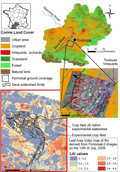
Figure 1. Location of the catchment area studied. The Auradé catchment comprises 101 cultivated crop fields. The cropping pattern is
a rotation of winter wheat and sunflower. The Formosat-2 series ground coverage is representative of the cropland area characterizing the region around Toulouse. Atmospheric turbulent fluxes, ground vegetation dynamics, and agro-meteorological measurements have been performed in the experimental crop field near the study site since 2005. A detail of the LAI map derived from the Formosat-2 image for 12 July 2009 shows the high variability of the LAI within the sunflower plots (still active at that period of the year), whereas other areas are close to zero, corresponding to winter wheat having reached the senescence stage.
agricultural area embedded within the Gascogne region in southwestern France, where a number of similar agricultural and geomorphologic settings are found (Ferrant, 2009). This small catchment (3.35 km2) is hilly and 88.5 % of its surface is cultivated. The substratum consists of impervious Miocene molasse deposits; a shallow aquifer, strongly heterogeneous in composition, overlies this argillaceous layer. Groundwater, sparsely distributed within sand lenses located at mid-slope and within deep alluvial soils bordering the stream network,
is the main source of the river’s discharge during low-flow periods.
The catchment’s soils were mapped in 2006 by Sol-Conseil and EcoLab; the map is presented in Ferrant et al. (2011). 12 soil types were identified along a topographic sequence, from deepest soil (around 2 m) in the bottomland to shallowest soils from middle slope to the top of slope (30 cm to 1 m). These agricultural soils exhibit low organic carbon (from 1.1 to 2 % in the first centimeter to 0.4 % in
deep horizons) and high clay contents (25 to 40 % in the first cm to 50 % in deep horizons). Each soil map unit rep-resents an area in which a specific soil type is dominant. Al-though the delineations are based on only 200 auger bore-holes in 325 ha, this map is nevertheless a reliable proxy for the fine variability of soil characteristics observed in the field. The climate is influenced by both the Oceanic and Mediterranean climates. Mean annual rainfall recorded on the study site for the 1985–2001 period was 656 mm, with a minimum of 399 and a maximum of 844 mm yr−1. The max-imum daily rainfall observed during this period was 90 mm; these intense rainfall events are seen during spring and au-tumn and generate large runoff events lasting less than 1 day. Average daily temperature was 14.5 ◦C, ranging from 0 to 1◦C in winter and 29 to 30◦C in summer, giving an av-erage potential evapotranspiration (PET) of 1020 mm yr−1.
The period 2006–2010 was marked by similar annual pre-cipitations: the mean was 664 mm yr−1, ranging from 628 to
737 mm yr−1, but hot springs and summers produced a higher PET (1039 mm yr−1). The annual discharge at the outlet is highly variable (from 6 to 33 % of the rainfall during the 1985–2001 period) and represents 4 to 15 % of the rainfall during the 2006–2010 study period. This period is drier in terms of hydrological conditions than the historical period used to calibrate the TNT2 model.
A hydrochemical database containing daily discharges and high-frequency nitrate concentration measurements was cre-ated and maintained by the AZF company from 1985 to 2001 and has been used to study nitrate contamination of the stream water at the catchment scale (Ferrant et al., 2011, 2013). Using this nitrate-oriented monitoring protocol, many more recent systematic observations and measurements were implemented to improve our understanding of the main pro-cesses that drive water, nutrient, and carbon fluxes in the agro-ecosystem and that are likely to be impacted by global changes.
1.6 Study period (2005–2010) and ground data 1.6.1 Hydro-chemistry
Stream-water nitrate concentrations and discharge were con-tinuously monitored at the outlet of the catchment during the 2005–2012 period (measurement protocol and data are fully described in Ferrant et al. (2012). From the continuous recorded signal, nitrate and water fluxes at the outlet of the catchment are aggregated to a daily time step to match the modeling time step.
1.6.2 Survey of agricultural practices
Annual inquiries about agricultural land cover and prac-tices are collected from volunteer farmers within the frame-work of the farmers’ association Association des agricul-teurs d’Auradé. Seeding dates, tillage operations, fertilizer
applications, crop harvest dates, and the amount of fertilizer applied constitute the basic agricultural practices reported by the farmers for each crop field. This cooperative survey never reaches 100 % participation, so many crop-field opera-tions remain unknown. For a given year, the missing seed-ing dates, fertilization amounts, and fertilization dates are deduced from existing recorded practices. A priori seeding dates are selected on the basis of the farmers’ annual re-ports. Only crop fields owned by a member of this associ-ation and located within the area of the municipality are in-cluded. Yields are also collected but frequently correspond to an average yield from several unidentified crop fields. This database is not exhaustive: for example, in 2006 only a third of the seeding dates are recorded for the whole municipal area, but none of the corresponding crop fields are included in the experimental catchment. In 2007, the seeding dates of only 18 crop fields among the hundred composing the catchment area are recorded. Expert opinion rules are used to fill the gaps in the database. For a given year, each miss-ing seedmiss-ing date is estimated by usmiss-ing the average seedmiss-ing date recorded for the crop fields owned by a farmer. If no seeding date is recorded for a crop field belonging to the farmer, the average of recorded seeding dates, computed for the crop type (wheat or sunflower) and for the year, is used. In this area, recorded winter wheat seeding dates may vary from the beginning of September to the end of November and sometimes even into December. Sunflower seeding dates vary from the middle of March to the end of April. This data reconstruction based on expert opinion rules is designed to find appropriate seeding dates based on farmer behavior and climatic years.
On the other hand, the crop rotation is known for the en-tire area during the study period. We compare the land cover information contained in the Registre Parcellaire Graphique (RPG) database with crop cover mapping using supervised classification of Formosat-2 and SPOT images. The RPG is based on annual farmer declarations of the land cover for crop-field blocks, a statement which is mandated by the Eu-ropean Common Agricultural Policy (CAP). However, both sources of information give the crop type (wheat, sunflower, rapeseed, barley) but no indication of the cultivar used. The main uncertainty in this agricultural database is linked to the seeding and fertilization dates, as well as to the amounts of fertilization. We refer to these agricultural practices data as “a priori” because they were compiled using non-exhaustive enquiries and used for a first run of the TNT2 model.
1.6.3 Turbulent atmospheric fluxes
Atmospheric flux instruments were set up in March 2005, lo-cated in an experimental crop plot 800 m beyond the eastern margin of the catchment (Fig. 1). Turbulent fluxes of CO2,
water vapor (actual evapotranspiration and latent heat), sen-sible heat, and momentum were continuously measured by the eddy covariance method (Baldocchi et al., 1988). Field
vegetation measurements were also performed to study the carbon balance and water use efficiencies of the crop-ping pattern (Béziat et al., 2009; Tallec et al., 2013). The daily actual AET measurements derived from this equipment will be compared with the AET simulated by the model for a similar crop location located inside the catchment.
1.6.4 Measurements of vegetation dynamics
Destructive measurements of vegetation dynamics were car-ried out on the experimental plot during each crop season of the study period. They consisted of estimating LAI and green area index (GAI) from aerial biomass measurements at the main development stages (Béziat et al., 2009). 10 and 30 plants were collected on two diagonals across the fields for wheat and sunflower, respectively. Sampling fre-quency was adapted to the vegetation development, from 1 month during the slow vegetation development period to 2 weeks during the fast development period. LAI and GAI were measured by means of a LI-COR planimeter (LI3100, LI-COR, Nebraska, USA). Between each destruc-tive measurement date, several randomly distributed hemi-spherical photographs were taken to capture the leaf devel-opment dynamics. The camera used for these measurements, a Nikon COOLPIX 8400 equipped with an FC-E8 fisheye lens, was placed on top of a pole to keep the viewing di-rection (downward-looking) and canopy-to-sensor distance (1.5 m) constant throughout the growing season. The hemi-spherical photographs were processed using CAN-EYE V5 (http://www4.paca.inra.fr/can-eye), which provides an effec-tive GAI (Baret et al., 2010; Demarez et al., 2008) for the whole image. These data were used to assess the model’s ac-curacy in reproducing the biomass production and LAI dy-namics of the crops. A field crop comparable to the experi-mental plot in terms of situation and cropping pattern was se-lected within the catchment: hereafter it is called crop field 8 (Fig. 1).
1.7 Leaf area index maps derived from Formosat-2 data
We used optical remote sensing data from Formosat-2 (F2; Chern et al., 2006) to estimate the LAI for each pixel of the ground coverage area (see Fig. 1). F2 is a high spatial (8 m) and temporal (daily revisit time) resolution satellite with four spectral bands (488, 555, 650, and 830 nm) and a swath of 24 km. For a given site, F2 data can be acquired every day with a constant viewing angle. This characteristic was used to perform accurate atmospheric corrections by estimating the aerosol optical thickness using a multi-temporal method (Hagolle et al., 2008). All F2 images were first pre-processed for geometric, radiometric, and atmospheric corrections, as well as cloud and cloud–shadow filtering (Hagolle et al., 2010).
105 LAI maps at 8 m resolution encompassing the whole catchment (ground coverage shown in Fig. 1) were derived from 105 Formosat-2 images over 5 years (2006–2010) us-ing the BV-NNET tool (biophysical variable neural network; Baret et al. (2007). BV-NNET is based on the inversion of a radiative transfer model (PROSAIL; Jacquemoud et al. (2009) using artificial neural networks. The LAI retrieval method is fully described in (Claverie, 2012, 2013). A main advantage of this method is that it does not require any prior calibration against in situ measurements.
The land cover within the experimental catchment was de-rived from field survey and F2 images by supervised classi-fication at the crop-field level. These map series were used to explore the spatial and temporal heterogeneity in terms of crop growth at the pixel and crop-field level. Daily values of LAI as a function of cumulative daily temperature were ob-tained by fitting a double logistic equation against discrete satellite-derived LAI (see equation in Fig. 2) at both crop-field and pixel levels. The results at the pixel level are used to discuss the spatial variability of the crop development ob-served within slopes and fields, whereas the results at the crop-field level are used in the optimization procedure de-scribed in Fig. 4.
1.8 TNT2 agro-hydrological model
TNT2 is a process-based, spatially distributed model devel-oped to study N fluxes and water cycles in small agricultural catchments (< 50 km2). The model combines the crop model STICS (Version 4) and the hydrological model TNT (Beau-jouan et al., 2002).
The TNT2 model has been successfully calibrated on the Auradé experimental catchment for the water and nitrogen fluxes at the outlet for a long period of time (1985–2001, Ferrant et al. (2011). TNT2 inputs and parameters include four types of spatial information: (i) a landscape pattern de-lineating the agricultural plots, roads, hydrological network, and landscape features (wetlands, hedgerows, etc.); (ii) a soil map; (iii) a climate map of climate gradients within the catch-ment; and (iv) agricultural practices associated with a crop sequence for each agricultural plot during the simulation pe-riod.
The TNT2 agronomical module is based on a STICS mod-eling approach (Brisson, 1998), a generic model that simu-lates crop growth at the plot scale using the input of agri-cultural practices: seeding date, crop cultivar characteristics, and mineral and organic fertilization. The crop plant is de-scribed by its shoot dry biomass (carbon and N), LAI, and the biomass of harvested crop organs. The cumulative air tem-perature is the main input variable driving crop growth: crop temperature is used to calculate the sum of degree days by phenological stage. Seeding date and first phenological stage lengths have a great impact on the crop emergence date and the entire LAI profile. Phenological stages are calibrated for each cultivar. One cultivar of wheat (Biensur) was selected
TNT2 Output LAI profile Input Seeding date T LAI Ti a Tf -b Kx Kn T LAI Tdiff Input +1
Seeding date - Tdiff
Tdiff_1 Tdiff_2 … Tdiff_n R1 R2 … Rn T Estimator: Tdiff ;RMSE LAI satellite interpolated Optimization process Iteration LAI=0.7
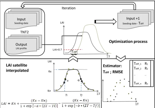
Figure 2. Process of optimization of the seeding date by matching the early variations of simulated LAI with the interpolated LAI derived
from F2 image series at crop-field scale. The interpolated LAIs are obtained by fitting a double logistic equation against discrete satellite-derived LAI at the crop-field scale. The equation describing the growth of the LAI depends on the cumulative daily temperature 6 T. Kn and Kx are the minimum and maximum of the interpolated LAI, respectively. Ti and Tf are the cumulative temperature when the LAI reaches Kx/2 during the growth and the senescence phases, respectively. Parameters a and b correspond to the local slope of the temperatures Tf and Ti.
(Brisson et al., 2002; Brisson, 1998). One cultivar of late sun-flower was calibrated for STICS (Brisson et al., 2003). Water and nutrient stress indices are associated with limitations re-garding leaf growth and the net photosynthesis of plants. The soil water and nitrogen contents simulated at a daily time step are combined with the daily crop requirements to compute the transpiration fluxes and nitrogen assimilation within crop biomass.
The water and N cycling in the soils is explicitly detailed by simulating evaporation (maximized by PET derived from a Penman–Monteith methodology) and transpiration, perco-lation to deep layers and lateral flows, organic matter min-eralization, mineral nitrogen denitrification (NEMIS model; (Henault and Germon, 2000; Oehler et al., 2009), and leach-ing into the hydrological network. The agricultural practices inputs are supplied at the crop-field level: seeding date, fertil-ization date and amount, straw management, and harvesting date.
The TNT2 hydrological module is a fully distributed hy-drological model, adapted to a topography-based shallow aquifer. It is based on the assumptions of the hydrologi-cal model TOPMODEL (Beven, 1997): water fluxes are as-sumed to follow Darcy’s law with a constant hydraulic gra-dient. The hydraulic transmissivity depends on the soil wa-ter deficit of saturation. The main differences between TNT and TOPMODEL lie in the distribution of the recharge and
the deficit of soil water saturation. TOPMODEL computes water fluxes at the outlet and an average deficit of satura-tion for the whole catchment, which can be distributed to each point of the basin according to a topographic index. In TNT, calculations are performed following an explicit cell-to-cell routing. The catchment is represented by a cluster of columns. Each top-of-column surface corresponds to a pixel in the digital elevation model (DEM). Each column height is divided into two soil layers corresponding to a root growth zone and a shallow aquifer layer. The soil and aquifer poros-ity is described as a dual porosporos-ity: the retention (micro) and drainage (macro) porosities. The porosity volume must be set up for each layer and for each soil type spatially delineated by the soil raster map. The water’s flow paths follow a multi-directional scheme (a pixel may flow into several other pix-els), which depends directly on the surface topography calcu-lated from the DEM. Water percolation and nitrogen leach-ing are computed usleach-ing cascadleach-ing horizontal layers similar to Burns’ model (Burns, 1974), according to soil porosity characteristics. Both the spatial soil characteristics and the multi-directional scheme derived from DEM define a spa-tially explicit distribution of recharge and deficit of soil water saturation. In addition to that, the cropping pattern and asso-ciated agricultural practices add spatial heterogeneity to this theoretical scheme in terms of water and nutrient transfers.
The model runs on a daily time step. Water balance and N transformations are computed for each cell of the raster grid of the DEM, from upstream to downstream, by follow-ing the cell-to-cell drainage routfollow-ing. Daily discharge and ni-trogen fluxes are computed at the outlet from the catchment.
1.9 Calibration of model
The model was calibrated for the period 1985–2001 firstly by optimization of the daily discharge using both hydrological parameters To and m, which influence the simulated hydro-graph characteristics: To is the lateral transmissivity of the soil column at saturation (in m2day−1)and m is the expo-nential decay factor of the hydraulic conductivity with depth (in meters). The Nash–Sutcliffe efficiency coefficient (Nash and Sutcliffe, 1970) was used as an optimization criterion to minimize mismatching for the daily discharge and nitrogen fluxes; RMSE was also used as a second performance indi-cator.
Using the same set of parameters as in Ferrant et al. (2011, 2013), we evaluated the simulations for the period 2005– 2010 in terms of hydrological and nitrogen fluxes, as well as the evapotranspiration and LAI/biomass data that were mea-sured in the experimental crop field (Fig. 1). We then used the F2 LAI data from 2006 to 2010 to perform the optimization process of the LAI.
1.10 Procedure for reassessing seeding dates
An algorithm designed to minimize temporal shifts between simulated LAI profiles and interpolated LAI profiles based on satellite images at the crop-field level was implemented (Fig. 2) to reassess seeding dates at the crop-field level. A first LAI profile is simulated for each crop field. Since the cumulative air temperature is the main input variable driving crop growth, the temporal shift (Tdiff)between the simulated
and interpolated LAIs is estimated in cumulative temperature (in◦C) for a threshold of LAI during the growth. The thresh-old is set to 0.7 because it avoids weed growth detection that could mislead the detection of the crop’s growth phase. Tdiff
is used to search for a second seeding date on the degree-day temporal scale by subtracting it from the first seeding date. A new Tdiff is computed on the simulation using the
sec-ond seeding date. 10 iterations of this optimization process described in the Fig. 2 were then performed. In addition to
Tdiff, the RMSE computed for the whole set of simulated and
observed LAIs is used to evaluate the optimization perfor-mance. No range of variation has been predefined because the next seeding date is computed by using the cumulative temperature differences.
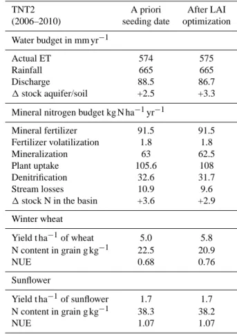
Table 1. Yearly water and N balance simulated in TNT2 model for
a priori and re-set seeding date.
TNT2 A priori After LAI
(2006–2010) seeding date optimization Water budget in mm yr−1
Actual ET 574 575
Rainfall 665 665
Discharge 88.5 86.7
1stock aquifer/soil +2.5 +3.3
Mineral nitrogen budget kg N ha−1yr−1
Mineral fertilizer 91.5 91.5 Fertilizer volatilization 1.8 1.8 Mineralization 63 62.5 Plant uptake 105.6 108 Denitrification 32.6 31.7 Stream losses 10.9 9.6
1stock N in the basin +3.6 +2.9
Winter wheat Yield t ha−1of wheat 5.0 5.8 N content in grain g kg−1 22.5 20.9 NUE 0.68 0.76 Sunflower Yield t ha−1of sunflower 1.7 1.7 N content in grain g kg−1 38.3 38.2 NUE 1.07 1.07 2 Results 2.1 Hydrological fluxes
Drainage and nitrogen fluxes simulated for the whole catch-ment are compared to the measurecatch-ments at the outlet. For this study, the hydrological calibration of input parameters pre-sented in Ferrant et al. (2011) is not modified. Similar perfor-mances are found for daily discharges (Nash–Sutcliffe coef-ficient E = 0.4). The annual average discharge for the period from May 2006 to December 2010 is around 71 mm yr−1, which is drier than the 107 mm yr−1estimated from 1985 to 2001. The simulated discharge is 88 mm yr−1between May 2006 and December 2010. This overestimation is compara-ble to that obtained for the dry years during the period 1985– 2001.
Observed in-stream nitrogen fluxes from January 2007 to December 2010 are close to 7 kg N ha−1yr−1, while simu-lated fluxes after LAI optimization are 9.6 kg N ha−1yr−1 (Table 1). The simulation performance is similar to that obtained for the calibration period published by Ferrant et al. (2011). The daily simulated nitrogen loads are poorly cor-related with observed data (R2=0.4), whereas correlation of monthly loads is higher (0.6). The RMSE for monthly loads
is 0.68 kg N ha−1yr−1. The hydrological control on daily
ni-trogen loads is poorly simulated. The comparison between the two similar agro-hydrological models SWAT and TNT2 suggests that one major reason behind these poor hydrologi-cal simulation performances is the dominant contribution of surface runoff to the discharge, which strongly impacts the NSE (Ferrant et al., 2011). These infra-daily fast transfers are strongly influenced by surface soil roughness, which is severely impacted by the argillaceous material composing the soil (40 %). Surface cracking during dry periods and pref-erential flow paths resulting from soil erosion are not taken into account in the daily estimation of runoff from the TNT2 modeling approach.
2.2 Leaf area index derived from Formosat-2 images
Figure 3a shows the maps of maximal LAI for each pixel, year, and crop. Figure 3b shows the LAI spatial variability observed for a sunflower crop field as a function of time: the spatial variability increases concomitantly with crop growth. This variability, expressed as the standard deviation (sigma), is of the same order of magnitude when considering variabil-ity between crop fields and within crop fields. The processes driving this spatial variability are mainly related to soil pat-terns, localization within slope, or aspect of the slope. The absolute value of LAI retrieval is compared with field mea-surements. Figure 4 compares two measurements of LAI: (1) RS LAI retrieved from satellite or hemispherical pho-tographs, and (2) direct measurement by the destructive method. Error bars represent plus or minus one standard de-viation of the median of the samples collected for the destruc-tive method. The variability of the result is associated with both the spatial variability of LAI and biomass encountered throughout the crop field and an imprecision attributed to the measurement method itself. The LAI estimated from hemi-spherical photographs is an average estimate for the whole area covered by the camera lens; error bars represent a fixed uncertainty related to this measurement method (Demarez et al., 2008). The satellite-derived LAI estimates for the crop-field level are represented by the median, plus or minus one standard deviation of the LAI value of each pixel located within the crop field. The error bar represents the spatial vari-ability detected by remote sensing.
The 44 cloud-free Formosat-2 images acquired in 2006 en-sure a fine-grained description of the winter wheat develop-ment. The intra-field LAI spatial variability obtained from the satellite retrievals is close to 1 m2m−2 during the
ma-turity stage. This spatial variability is estimated to be higher for the sunflower in the following year (2007) with an LAI of 1.5 (Fig. 4). In 2008, the presence of clouds during the spring prevented observation of winter wheat growth, whereas im-ages taken during the summer allowed a survey of sunflower growth. These results illustrate the intrinsic accuracy of each measurement method and the spatiotemporal variability of
the crop growth. The F2 spatial resolution and high revisit frequency enable us to capture the growth dynamics.
2.3 Optimizing LAI profile
Figure 5 shows the results of optimizing the temporal dy-namics of the LAI average over the 101 crop fields. Reini-tialization of the seeding dates decreases the temporal shift (Tdiff)by a factor of 7 on average. The optimized simulated
LAI profiles correspond better with the observed data for each wheat growing period. The differences for the sunflower are small since the temporal shifts between interpolated ob-servations and simulated LAI were already small. This in-dicates that the first-guess seeding dates for the sunflower were accurate. A slight decrease of RMSE is observed af-ter optimization, meaning that this estimator is not sensitive to the seeding date reassessment. In fact, the RMSE value is representative of the whole LAI series, whereas the op-timization process takes only the early phenological stages into account. Furthermore, the senescence stage of the win-ter wheat is not correctly simulated: afwin-ter the maximum is reached, simulated LAI remains stable until the harvest. The observed LAIs from satellite data are derived from photo-synthetic activity, which decreases early on when the wheat becomes dry. This portion of the development is better de-scribed in the last release of STICS 6.
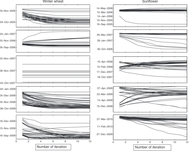
The trajectories of seeding date solutions as a function of the iteration number (Fig. 6) show a rapid convergence after five iterations. There are few crop fields for which no real-istic solutions were reached. For the sunflower in 2007, four crop fields converged on an early seeding date in October to December. This exclusively concerns the sunflower in cer-tain small crop fields (several hectares) for which average LAI remains low (< 1). In these cases, the maximum of ob-served LAI is too low or the proportion of mixed pixels (at the crop-field border) is too high, thereby leading to unreal-istic interpolations of the LAI profile at the crop-field level. The annual seeding dates estimated by this method constitute a long period for the winter wheat and a short one for the sun-flower. These ranges are from September to the beginning of November for winter wheat and between January and April (highly dependent on the climatic year) for the sunflower. In 2007, 2008, and 2010 the seeding dates for winter wheat and sunflower crop fields were recorded within the experimental catchment. The average differences between estimated and actual seeding date in 2007 were 20 and 8 days for the wheat and sunflower crops, respectively. These figures rise from 1 day to 1 month and from 1 to 17 days for wheat and sun-flower, respectively. Three factors are responsible for these heterogeneous differences: inappropriate cultivar growth pa-rameters, inaccurate detection of emergence period by biased LAI interpolation from remote sensing, and uncertainties in farmer statements (completed at the end of each year).
Figure 3. Above: maps of maximum LAI observed for each year and each crop mask. Maxima of winter wheat LAI were not observed
during spring 2008 owing to heavy cloud cover throughout the area. Each date of image acquisition constituting the F2 series is indicated by a triangle in the timeline. Below: spatial variability of the LAI as a function of the time between (inter-sigma) and within (intra-sigma) crop-field measurements for sunflower.
2.4 Sensitivity of discharge and stream nitrogen fluxes to seeding date
Table 1 presents the annual water and nitrogen fluxes com-puted for the entire simulation period (2006–2010). The changes in crop development induced by the reinitialization of input parameters have a small effect on the discharge and AET (around 1 to 2 mm yr−1). On the other hand, the global nitrogen uptake by the crop is increased in the case of seeding date reinitialization (+3 kg N ha−1yr−1). This leads to a decrease of in-stream nitrogen fluxes at the outlet to 9.6 kg N ha−1yr−1, which is closer to the annual N fluxes measured at the outlet (7.5 kg N ha−1yr−1). The yields of wheat crops are more strongly impacted by the seeding date reinitialization than those of the sunflower (Fig. 5); the wheat yield increases from 5 to 5.8 t ha−1, whereas it remains
sta-ble for the sunflower. This optimization process increased the nitrogen-use efficiency (NUE) of wheat as well. The ratio of nitrogen uptake by the plant to nitrogen input by fertilizers seeks to measure the efficiency of agricultural practices. It shows that the N inputs from fertilization are better absorbed by the plants. Nevertheless, the N content in grain ratio is slightly decreased, since it depends both on grain biomass and on the N content of grain. The sunflower yield is not
im-pacted since the LAI profiles were not really altered by the reinitializing of the seeding date.
2.5 Impact at a crop-field level
Figure 7 shows the results of seeding date reinitialization on the LAI and biomass estimates, respectively. We compare two crop fields: one is located within the catchment where TNT2 simulations are performed (crop field 8) and the other is the experimental crop field where measurements of tur-bulent atmospheric fluxes are carried out (see Fig. 1). The crop fields are close to each other and comparable in terms of slopes and crop rotation, except in 2009 when rapeseed crop was grown in the experimental field and sunflower was sown in crop field 8, located within the catchment. Remotely sensed LAI values for both crop fields are compared to il-lustrate the differences observed between the crops in terms of vegetation dynamics. The interpolated daily LAI is pre-sented in Fig. 7 for the crop within the catchment, and the simulated LAI profiles before and after the optimization are plotted. The simulated biomasses before and after optimiza-tion in crop field 8 are compared to the measured biomass within the experimental crop field. The spatiotemporal vari-ability of this variable is close to the measurements for the
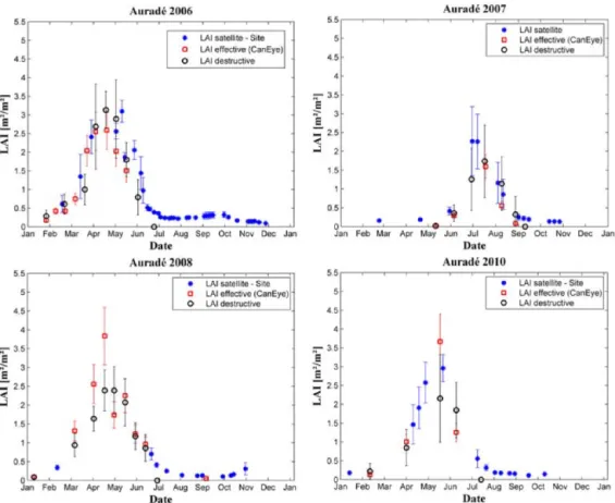
Figure 4. Leaf area index derived from satellite F2 images, hemispherical photographs (LAI effective CanEye), and direct field measurement
(LAI destructive) in the experimental crop field located near the Auradé catchment (see location in Fig. 1). The standard deviation represents the spatial variability within the crop field (LAI satellite), spatial variability and associated sampling error (LAI destructive), and uncertainty concerning the photo interpretation (LAI effective).
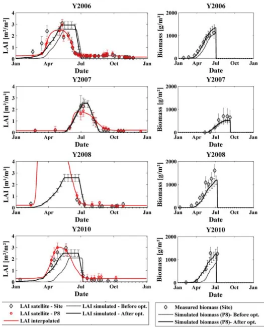
4-year period, except in 2008 when no optimization could be performed because of heavy cloud cover. The seeding date modifications have a substantial impact on biomass produc-tion and clearly improve the biomass predicproduc-tions for 2010.
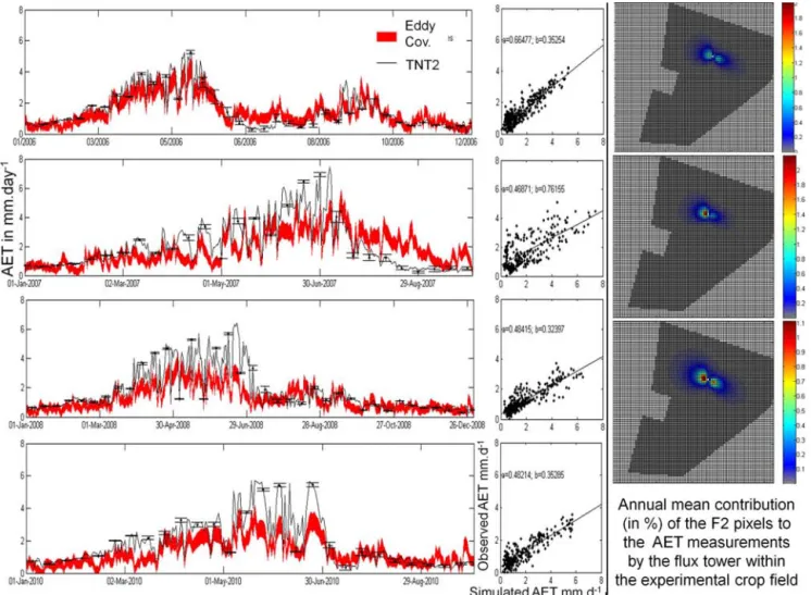
Figure 8 compares the daily simulated and measured evap-otranspiration fluxes at the crop field 8 and experimental crop-field levels. Each series is strongly correlated in time (R>0.7), which means that the climatic control of the AET is conveniently accounted for. In contrast, the Nash–Sutcliffe coefficient E, usually employed for hydrological flux evalua-tion, exhibits high inter-annual variability: from a good cor-respondence between flux measurements and simulations in 2006 (E = 0.57) to a negative value in 2007, 2008, and 2010. It shows that bias is high; cumulative annual measured AET tends to be overestimated by the simulations: by 11 and 15 % in 2006 and 2007 and by more than 30 % in 2008 and 2010. The RMSE of each series is around 1 mm day−1 except for the year 2006, when it is half as large. Figure 8 shows the un-certainty associated with the random measurement errors for semi-hourly fluxes as an envelope around the daily AET and indicates that it is roughly proportional to the flux intensity (Béziat et al., 2009). Eddy covariance measurements are rep-resentative of a fluctuating area (called the footprint) of the
crop field, which varies mainly with the crop-cover height, wind speed, and direction. The footprint, corresponding to the area which is contributing to the measurements made at the tower location, was computed in a previous unpublished study using both half-hourly climatic variables measured lo-cally and a footprint model (Horst, 1999). Figure 8 (right) shows the average footprint area for the years 2006, 2007, and 2008, estimated by the footprint model, climatic data, and crop height measured in the experimental crop field. It shows the total contributive area and the location of high contributive areas (yellow and red colors). Two main wind directions explain the footprint’s symmetry on either side of a WNW–ESE axis. The main contributive area remains close to the flux tower; the footprint in 2006 is more homo-geneous and wider than those in 2007 and 2008. Average footprint areas are close to the flux tower, which is not rep-resentative of the entire experimental crop field; moreover, the footprint area is located in a zone characterized by shal-low soil depth associated with shal-low crop productivity. These AET measurements may therefore represent the low bound-ary of the AET range within the plot. TNT2 estimates at the crop-field (8) level are systematically higher than the in-field measurements, but the spatial variability within the crop field
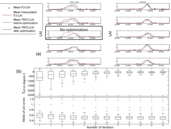
Figure 5. (a) Average LAI computed at the crop-field level for winter wheat (left) and sunflower (right) for each year of simulation (lines).
Simulated LAIs before and after the optimization process are shown in dashed and full black lines, respectively. Average crop-field level LAIs retrieved from F2 images are represented by black circles and the average interpolations from these images are shown by full red lines.
(b) Evolution of Tdiffin degree days and RMSE found for each crop as a function of the number of optimization process iterations. The first and third quartile and the median of Tdiffand RMSE for each crop field are shown. Red crosses stand for outliers.
(represented by paired bars of standard deviation every 10 days) ranges between 0.4 and 1.8 mm day−1during the crop-growing season (spring and summer). This spatial variability is as high as the RMSE found for both the observed and sim-ulated series. Unfortunately, comparison between observed and simulated AET cannot be performed for the footprint area only, since the crop fields are separated by a distance of 800 m.
3 Discussion
3.1 LAI profile improvement
Field measurements of LAI or AET are expensive, time-consuming, and limited to local evaluations of the crop cover. The satellite observations are thus essential for monitoring the crop-cover dynamics at crop-field scales. In the context of the present study, leaf area index and biomass are highly
variable in space and time and within crop field. The high spatial resolution (around 10 to 20 m) is sufficient to cap-ture the spatial variability of crop productivity. The large number of images, provided by the high frequency of satel-lite revisit, makes it possible to describe the temporal crop development and productivity at pixel and crop-field levels by describing the LAI profile retrieved from F2 images by means of a physically based double logistic descriptive equa-tion (Fig. 2). This temporal informaequa-tion has been used at the crop-field level to optimize the simulated LAI of the process-based model STICS, coupled with a hydrological model that aims to reproduce the varying local situations created by hy-drological conditions within the catchment. The objective of minimizing the temporal shift between measured and ob-served LAI by re-initializing the seeding date in TNT2 is satisfactorily fulfilled: there is a rapid convergence of the op-timization process, with temporal shifts being generally min-imized with a realistic seeding date solution. The improve-ment achieved from the a priori situation constructed from
04−Oct−2005 03−Nov−2005 Winter wheat 16−Sep−2005 15−Nov−2005 14−Jan−2006 15−Mar−2006 14−May−2006 Sunflower 26−Sep−2006 25−Nov−2006 24−Jan−2007 30−Oct−2006 28−Jan−2007 29−Mar−2007 25−Oct−2007 08−Nov−2007 23−Nov−2007 18−Oct−2007 17−Dec−2007 15−Feb−2008 15−Apr−2008 06−Oct−2008 05−Nov−2008 05−Dec−2008 04−Jan−2009 15−Dec−2008 14−Apr−2009 23−Mar−2009 27−Apr−2009 0 2 4 6 8 10 12 16−Sep−2009 15−Nov−2009 18−Dec−2009 0 2 4 6 8 10 12 27−Dec−2009 11−Feb−2010 27−Mar−2010
Number of iteration Number of iteration
Figure 6. Seeding date trajectories for each crop field as a function of iteration number.
the local database would have been made more evident by constructing a seeding-date scenario based on regional rec-ommendations. This could be done in future applications at larger scale, e.g., by considering ground coverage of com-plete Formosat-2 scenes.
3.2 Seeding date estimation
Nevertheless, although seeding-date values are a good nu-merical solution for phasing simulated and RS-retrieved LAI profiles, final seeding-date values mainly depend on the cul-tivar parameters, such as length of the early development and vernalization stages. For instance, the duration of winter wheat vernalization, corresponding to the low temperature periods required to hasten plant development, will depend on the number of vernalizing days defined for each wheat cultivar (JVC parameter) and the crop temperature computed from climate input data. The mild winter conditions in the study area make the LAI profile insensitive to the seeding date for high values of JVC (> 8). We have therefore set the JVC parameter to 6 days for the winter wheat cultivar used in this study. This shows that the variety of wheat sown is crucial information for a better estimation of the true
seed-ing date, crop-growth dynamic, and yield. More generally, crop variety is not recorded in an agricultural database. In this specific study site, several varieties were recorded which were not pre-calibrated in the STICS model. The estimation of a “true seeding date” at catchment scale is accordingly not possible at present.
3.3 Optimization process performance
Jégo et al. (2012) used LAI data retrieved from satellite im-ages to better constrain input parameters for the STICS crop model. By reinitializing the seeding date, they greatly im-proved the model’s predictions in terms of biomass and yield. The optimization method is based on the simplex algorithm to minimize the weighted sum of squared differences be-tween RS-retrieved and simulated LAI series. A run of the crop model is carried out for 1 crop and 1 year and takes less than a second. This optimization method is appropriate since it tests several input parameter couples in order to con-verge quickly on an optimal solution in terms of the cho-sen estimator. In the case of TNT2, simulations are sequen-tially executed: each pixel calculation depends on the pre-vious and simulated neighborhood conditions. A single run
Figure 7. LAI and biomass simulated for 4 years in the crop within the catchment that exhibits a cropping pattern comparable to the
experimental crop field (except in 2009) where the ground measurements are carried out. Rows stand, respectively, for winter wheat 2006, sunflower 2007, winter wheat 2008, and winter wheat 2010. LAI in the first column: the red curve is the interpolated LAI profile from the F2-derived values (red circles) with the spatial variability represented by the bars. The black diamonds represent the F2–LAI values for the experimental crop field located outside the catchment. Black solid and dotted lines are the average LAI after and before seeding date modification, respectively; bars represent the standard deviation of simulated LAI within the crop field. Biomass in the second column is represented by black diamonds for the measurements, with the measurement variability associated with the spatial variability and accuracy of the measurement method. Black solid and dotted lines are the average biomass after and before seeding date modification, respectively; bars represent the standard deviation of simulated LAI within the crop field.
corresponds to the simulation of water and nutrient fluxes in 134 013 modeling units, covering 101 crop fields for 5 years. It thus requires much more computation time (around 2 h for the Montoussé river catchment). The hydrological interac-tions between modeling units in space and time imply that changes in seeding dates are interdependent. The optimiza-tion method described in this paper was chosen because it is based on a quantitative (rather than a statistical) estimator
of the temporal shifts, which is used to quantitatively cor-rect the input parameter (in this case the seeding date) based on the model’s functioning. The temporal delay between RS-retrieved and simulated LAI series is evaluated as a physical variable: the cumulative daily air temperature difference. The results of this optimization show a rapid convergence after five to eight iterations.
Figure 8. Left: measured versus simulated daily actual evapotranspiration from the experimental crop field and crop field 8, respectively.
Measured AETs are given with the uncertainty envelope associated with the eddy covariance measurement precision (Béziat et al., 2009). The Nash–Sutcliffe coefficient, correlation coefficient (without units), and RMSE (mm day−1) are, respectively, 0.57, 0.9, and 0.57 for the year 2006; −0.24, 0.7, and 1.18 for 2007; −0.6, 0.87, and 1 for 2008; and −0.68, 0.88, and 1 for 2010. Linear regressions of the form Obs = a × Simulated + b are shown for each year. Right: average annual footprint of the flux tower within the experimental crop field, computed by the model of Horst (1999). Colors stand for the contribution of each pixel to the AET measured at the tower level (in percentage). Pixel contributions in 2006 are more homogeneously distributed within the footprint than in 2007 and 2008 (unpublished study by E. Potier).
3.4 Impact of re-initializing on agro-hydrological variables
The STICS crop model (the agronomical portion of the TNT2 model) is a process-based model, i.e., it is able to scale up the results of local experiments. It extrapolates the crop-growth variables from analogous situations described by in-put data (soil, climatic, and cropping management) with-out the need for new testing. The coupling of this process-based model with a hydrological model seeks to simulate the varying local situations described by hydrological con-ditions within the catchment: saturated zones and soil water content as a function of the situation within a slope. The hy-drological variables – evapotranspiration and discharge – are not heavily impacted by this change in crop-cover dynamics.
The difference obtained for AET, i.e., 2 mm yr−1, is similar to the impact of systematic catch crop implementation be-tween wheat and sunflower that was tested in this catchment using TNT2 for the period 1985–2001 (Ferrant et al., 2013). Nevertheless, an improvement of the AET simulation is still needed to confirm this result. On the other hand, the improve-ment of the representation of crop-cover dynamics obtained by reinitializing the seeding date has a substantial impact on wheat biomass production (Fig. 7) and associated nitrogen uptake: NUE and yield of winter wheat are mainly increased by the reinitializing process. Thus, simulated nitrogen fluxes into the environment decrease by 2.7 and 11.9 % for denitri-fication and stream losses, respectively. Being dynamically controlled by the discharge, in-stream nitrogen fluxes
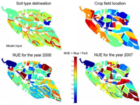
simu-Figure 9. Soil and crop-field map used in TNT2 (top). Spatial NUEs for the years 2006 and 2007 (bottom left and right, respectively). The
higher the value, the more efficiently the fertilizer is used by the plant. A low fertilizer amount with weak biomass production could lead to high NUE. Mineralization of soil organic matter creates a source of mineral nitrogen that leads to NUEs higher than unity.
lated over a long period depend strongly on the balance be-tween fertilizer applications and crop consumption. In this case, average annual simulated nitrogen fluxes were lowered from 11 to 9.6 kg N ha−1yr−1, which is in better agreement with the 7.5 kg N ha−1annual estimation based on intensive measurements. In general, the improvement of the spatial and temporal crop cover and nitrogen uptake representation would improve our understanding of the N cycle by estimat-ing the locations of nitrogen excesses and associated poten-tial losses into the hydrologic and atmospheric systems. The mapping of the NUE in 2007 is presented in Fig. 9. By dis-playing the ratio between nitrogen fertilizer input (crop-field level) and plant uptake (at pixel scale), it indicates the ar-eas where plant uptakes exceed N inputs (NUE > 1) and the areas contributing to N losses where N inputs exceed plant uptake (NUE < 1). These representations of nitrogen excess in the landscape will definitely benefit from a crop develop-ment optimization at the pixel level using LAI derived from RS image series.
3.5 Input parameter (soil and hydromorphy) and spatial representation of hydrological situations
Other input parameters than the seeding date should be con-sidered for further optimizations. Jégo et al. (2012) have identified a second input parameter known to have a great im-pact on crop productivity within the STICS crop model: the soil’s water-retention capacity. In the TNT2 model, the soil map defines homogeneous zones where 21 soil parameters
are defined. The sensitivity of the spatial pattern of soil in-put parameters within agro-hydrological models has not yet been deeply explored. Figure 8 shows the spatial variabil-ity of the F2-derived and TNT2-simulated LAI at the pixel level for two dates. Two covariates seem to drive the spatial variability of the LAI variations simulated by TNT2: the soil map and the location of the drainage network. Three main situations are simulated: (1) systematic saturated conditions, which limit LAI development in the drainage network lo-cation; (2) low soil water deficit, which enhances LAI de-velopment; and (3) intermediate or low soil water content, which limits LAI development. There is an excellent poten-tial for agronomical calibration of agro-hydrological models by reinitializing soil input parameters and refining local sit-uations at the pixel scale, using these new LAI map series derived from optical RS with high revisit frequency. Consid-ering only the hydrological variables, Moreau et al. (2013) tested the sensitivity of the TNT2 model’s response to spa-tial soil input parameters for both water and nitrogen-related parameters. They analyzed the output’s sensitivity in terms of in-stream water and nitrogen fluxes at the outlet and con-cluded that sensitivity to the spatial distribution of soil input factors is low. Looking ahead, we consider that the sensitiv-ity of spatial soil input parameters is high for crop variables and would impact the spatial representation of the N cycle within slopes. Reinitialization of physical soil parameters in the TNT2 model will be proposed in a forthcoming study at the pixel level using the same F2 data set. The control of these parameters versus other physical catchment parameters
(aspect, slopes, etc.) on the spatial and temporal variability of the crop growth will be explored.
4 Conclusions
The present study has evaluated the potential of remote sensing data series for the spatial and temporal calibra-tion of a distributed agro-hydrological model over a 5-year period (2006–2010). The use of a process-based crop model (STICS) coupled with a simplified hydrological model (TNT) provided the means to simulate the water and nitrogen budgets as well as the yields of a soil–plant system at the catchment scale, taking climatic and agricultural variables into account. The lack of spatial and temporal calibration of soil–crop situations is assessed in light of the additional spa-tiotemporal information derived from RS images. The spatial calibration of model input parameters by using LAI derived from RS image series, previously confined to a priori values, opens new opportunities for constraining spatial and tempo-ral crop development at the catchment scale. In this exam-ple, we satisfactorily constrained the temporal LAI develop-ment at the crop-field level by reinitializing the seeding dates. This calibration step adds value to the conventional calibra-tion process usually employed in agro-hydrological models. The improved representation of crop-cover growth has no no-ticeable impact on the water budget at the catchment scale (around 1 %), but had substantial impacts on the nitrogen cy-cle in terms of crop uptake and biomass, as well as on nitrate leaching and in-stream losses. The optimization process us-ing RS-derived LAI profiles has enabled an increase in nitro-gen uptake by the crop and in biomass production for winter wheat, leading to a significant drop in the simulated in-stream nitrogen losses of around 12 %. This result indicates that a spatial calibration of the crops’ biophysical variables such as LAI changes the nitrogen-use efficiency (NUE) at the crop-field level, which impacts the nitrogen cycle at the catchment scale.
This study demonstrates the contribution of high spatial resolution optical satellite images with frequent systematic observations to the spatial calibration of agro-hydrological models. This type of spatial calibration greatly improves the capacity of agro-hydrological modeling to explain, repro-duce, and predict spatial crop growth by constraining the spatial water and nutrient fluxes within a hydrological catch-ment. Massive systematic satellite observations will soon be-come widely available thanks to the forthcoming satellite missions Venµs (Dedieu et al., 2007) and Sentinel-2, which will provide high spatial resolution images with a 4-to-5-day revisiting frequency. Further development will test a similar reinitialization algorithm on the main soil parameters con-trolling soil water content so as to improve the simulated LAI profile at the pixel level.
The Supplement related to this article is available online at doi:10.5194/hess-11-5219-2014-supplement.
Acknowledgements. We would like to thank the Association des
Agriculteurs d’Auradé (today Groupement des Agriculteurs de la Gascogne Toulousaine) for their cooperation and the people who are behind the large amount of data presented in this manuscript: Nicole Ferroni, Bernard Marciel, Pascal Keravec, Hervé Gibrin, Tiphaine Tallec, Pierre Béziat, Pierre Adrien Solignac, Aurore Brut, Jean-François Dejoux, Claire Marais-Sicre, Jérôme Cros, Olivier Hagolle and Mireille Huc. Nitrate concentration and stream discharge were recorded within the framework of a GPN-ECOLAB convention on the experimental catchment of Auradé. The BVEA (Bassin Versant Expérimental d’Auradé) is a regional platform of research and innovation in Midi-Pyrénées and innovation and which is involved in the French SOERE Network RBV (Experi-mental catchment network) and in the international Critical Zone Exploratory Network. Sylvain Ferrant was the recipient of a CNES (Centre National d’Etudes Spatiales) post doctoral research grant. Edited by: V. Andréassian
References
Arnold, J. G., Allen, P. M., and Bernhardt, G.: A comprehensive surfacegroundwater flow model, J. Hydrol., 142, 47–69, 1993. Arnold, J. G., Srinivasan, R., Muttiah, R. S., and Williams, J. R.:
Large-area hydrologic modeling and assessment: Part I. Model development, J. Am. Water Ressour. Assoc., 34, 73–89, 1998. Baldocchi, D., Hicks, B., and Meyers, T.: Measuring biosphere–
atmosphere exchanges of biologically related gases with mi-crometeorological methods, Ecology, 69, 1331–1340, 1988. Baret, F., Hagolle, O., Geiger, B., Bicheron, P., Miras, B., Huc, M.,
Berthelot, B., Nino, F., Weiss, M., Samain, O., Roujean, J. L., and Leroy, M.: LAI, fAPAR and fCover CYCLOPES global products derived from VEGETATION, Part 1: Principles of the algorithm, Remote Sens. Environ., 3, 275–286, 2007.
Baret, F., De Solan, B., Lopez-Lozano, R., Ma, K., and Weiss, M.: GAI estimates of row crops from downward looking digital pho-tos taken perpendicular to rows at 57.5 degrees zenith angle: the-oretical considerations based on 3D architecture models and ap-plication to wheat crops, Agr. Forest Meteorol., 150, 1393–1401, 2010.
Beaujouan, V., Durand, P., Ruiz, L., Aurousseau, P., and Cot-teret, G.: A hydrological model dedicated to topography-based simulation of nitrogen transfer and transformation: rationale and application to the geomorphology-denitrification relationship, Hydrol. Process., 16, 493–507, 2002.
Beven, K: Distributed modelling in hydrology: applications of top-model concept, Adv. Hydrol. Process., 350, 1997.
Beven, K: Equifinality, data assimilation, and uncertainty esti-mation in mechanistic modelling of complex environmental systems using the glue methodology, J. Hydrol., 249, 11–29, doi:10.1016/S0022-1694(01)00421-8, 2001.