Designing RNA Secondary Structures is NP-Hard
Édouard Bonnet1, Paweł Rzążewski2, and Florian Sikora3
1Middlesex University, Department of Computer Science, London, UK [email protected]
2Faculty of Mathematics and Information Science, Warsaw University of Technology, Warsaw, Poland [email protected]
3Université Paris-Dauphine, PSL Research University, CNRS, LAMSADE, Paris, France [email protected]
Abstract
An RNA sequence is a word over an alphabet on four elements {A, C, G, U } called bases. RNA sequences fold into secondary structures where some bases match one another while others remain unpaired. Pseudoknot-free secondary structures can be represented as well-parenthesized expressions with additional dots, where pairs of matching parentheses symbolize paired bases and dots, unpaired bases. The two fundamental problems in RNA algorithmic are to predict how sequences fold within some model of energy and to design sequences of bases which will fold into targeted secondary structures. Predicting how a given RNA sequence folds into a pseudoknot-free secondary structure is known to be solvable in cubic time since the eighties and in truly subcubic time by a recent result of Bringmann et al. (FOCS 2016), whereas Lyngsø has shown it is NP-complete if pseudoknots are allowed (ICALP 2004). As a stark contrast, it is unknown whether or not designing a given RNA secondary structure is a tractable task; this has been raised as a challenging open question by Anne Condon (ICALP 2003). Because of its crucial importance in a number of fields such as pharmaceutical research and biochemistry, there are dozens of heuristics and software libraries dedicated to RNA secondary structure design. It is therefore rather surprising that the computational complexity of this central problem in bioinformatics has been unsettled for decades.
In this paper we show that, in the simplest model of energy which is the Watson-Crick model the design of secondary structures is NP-complete if one adds natural constraints of the form: index i of the sequence has to be labeled by base b. This negative result suggests that the same lower bound holds for more realistic models of energy. It is noteworthy that the additional constraints are by no means artificial: they are provided by all the RNA design pieces of software and they do correspond to the actual practice (see for example the instances of the EteRNA project). Our reduction from a variant of 3-Sat has as main ingredients: arches of parentheses of different widths, a linear order interleaving variables and clauses, and an intended rematching strategy which increases the number of pairs iff the three literals of a same clause are not satisfied. The correctness of the construction is also quite intricate; it relies on the polynomial algorithm for the design of saturated structures – secondary structures without dots – by Haleš et al. (Algorithmica 2016), counting arguments, and a concise case analysis.
1
Introduction
Ribonucleic acid (RNA) is a molecule playing an important role between deoxyribonucleic acid (DNA) and proteins. RNA is a chain of nucleotides (or bases) and can be represented as a sequence
on a 4-letter alphabet: A, U, C, G; denoting the first letter of the corresponding nucleotide. Unlike DNA, RNA is single stranded, and folds into itself: some of the bases are linked to each other (they are paired or matched) to form a stable and compact structure. This pairing forms the secondary structure of the RNA molecule; the primary structure is the sequence of nucleotides and the tertiary structure is the 3D shape. Predicting how an RNA molecule folds is vital to understand its biological function.
Experiments reveal that the secondary structure of an RNA strand tends to follow the laws of thermodynamics. Given a model associating a free-energy value to secondary structures, it is widely accepted, since the pioneer work of the chemistry Nobel laureate Christian B. Anfinsen [5], that the secondary structure of a sequence can be predicted as the one with the minimum free-energy (MFE), i.e., the one ensuring the greatest stability. The most simple energy model is the Watson-Crick model, allowing A to pair with U and C to pair with G. In this model, the MFE is simply realized by a structure with the greatest number of pairs.
RNA folding. A stem-loop or hairpin loop is a building block of RNA secondary structures. It
consists of a series of consecutive base pairs (called double-helix or stackings) ending in a loop of unpaired nucleotides. A pseudoknot occurs when some nucleotides of this loop pair somewhere else in the RNA strand. Pseudoknot-free secondary structures correspond to well nested structures. They can be represented as a well-parenthesized expression where matching parentheses symbolize base pairs, with additional dots to symbolize unpaired nucleotides.
Given a sequence of nucleotides, the RNA Folding problem consists of finding the pseudoknot-free secondary structure with the minimum pseudoknot-free-energy. RNA Folding can be solved by a simple
dynamic programming in time O(n3) where n is the size of the sequence [24, 32]. Since this
result in the early 1980s, a lot of work has been devoted to propose new methods for secondary structure prediction. Recently, the first truly subcubic algorithm for RNA Folding was proposed
by Bringmann et al. [8] and runs in deterministic time O(n2.861) or randomized time O(n2.825).
Some faster polynomial-time approximation algorithms were later obtained [27].
When pseudoknots are allowed, the computational complexity of predicting how RNA folds gets a bit blurry. The short answer would be to say that the folding prediction becomes NP-complete [2, 18, 23]. Observing that none of those three hardness constructions are ideal, the first one because the value of the free-energy is not fixed but specified as part of the input, and the other two, because they assume that only planar pseudoknots are legal, Lyngsø gives two additional NP-hardness proofs [22]. They work in seemingly very close models; both not too distant from Watson-Crick. However, the NP-hardness in one model crucially needs that the alphabet size is unbounded (which is rather unsatisfactory), while the NP-hardness in the other model carries over to a binary alphabet. When only restricted types of pseudoknots are allowed, dynamic programming still works and yields polynomial-time algorithms with worst running times than in the pseudoknot-free case [2, 10, 23, 25]. Under the hypothesis that the pseudoknots may only form after the pseudoknot-free pairs, the O(n3)-time complexity can be attained again [19]. In a simpler model, an approach based
on maximum weighted matchings makes the folding prediction tractable for general pseudoknots [29].
RNA design. In the inverse folding problem called RNA Design, one is given a secondary
structure and has to find a sequence of bases which uniquely folds into this structure; or report that such a sequence does not exist. The sequence must fold into this structure preferentially to any other structure. In particular, in the Watson-Crick model, any other structure the sequence can fold into must have strictly less pairs. If such a sequence exists, we call it a design for the secondary
structure.
This problem was introduced in the early 1990s in a paper which, to date, has over 2000 cita-tions [17]. Surprisingly, the complexity of RNA Design is still unknown despite two decades of works and was explicitly stated as a major open problem [4, 12, 13, 16, 21]. This is exceptional for a central problem in computational biology [16]. Schnall-Levin et al. gave a NP-hardness proof for a more general problem [28]. However, to be applicable to RNA Design, the energy model would have to depend on the 3-Sat instance in the reduction (hence, would be different for each instance) which is clearly not realistic (see the discussions in [16, Section 5] or in [21]).
Solving RNA Design finds applications in multiple fields such as pharmaceutical research and biochemistry [16] as well as synthetic biology and RNA nanostructures [11]; the two latter areas aim at creating enhanced RNA with desirable properties. It is also a major step towards functional
RNA molecular design. Therefore, there are many algorithms and software products1 solving the
RNA inverse folding problem [1, 4, 9, 14]. Churkin et al. compare the main freewares solving RNA Design such as RNAInverse, antaRNA, and RNAiFold [11]. All of them are either heuristics, or use meta-heuristics, or have an exponential running time. Let us also mention the EteRNA project, an online game where (more than 100.000) players have to find a correct sequence given a structure [20]. In 2016, some expert players have solved hard instances that known algorithms could not solve [3]. Recently, Haleš et al. gave some sufficient conditions under which one can answer to the problem in polynomial time [16]. Their main result is to show that if the structure is saturated, i.e., does not contain any unpaired letter, then a design –if it exists– can be found in linear time by a greedy procedure. In the case of saturated structures, the existence of a design is solely based on the maximum degree of a tree representing the structure. The authors also show that on smaller alphabets and general secondary structures, RNA Design is tractable.
Following the name of the precoloring extension problem in graphs [6], let the extension version (RNA Design Extension) of the inverse folding problem be the same as RNA Design with the additional constraint that some indices of the RNA sequence should contain a specified base. Lyngsø observes that this assumption is biologically coherent: “Most recent methods do allow for position specific constraints, where in addition to folding into the target structure the designed sequence is also required in certain positions to have a particular nucleotide” [21]. Indeed, in addition to the target structure, one has to force some bases at key positions to ensure that the RNA molecule possesses a given function. Zhou et al. also propose a method to solve RNA Design where some positions within the sequence are constrained to certain bases [31]. Rodrigo et al. impose the presence of a certain sequence at a specific position in the structure [26]. Borujeni et al. enforce the presence of a given subsequence (called the Shine-Dalgarno sequence) paired to a “start codon” to start the translation of RNA to proteins [7]. Furthermore, software libraries solving RNA Design allow those additional unary constraints and the instances of the EteRNA project contain immutable nucleotides. Thus it appears that the design of RNA secondary structures is better captured by RNA Design Extension than its restriction RNA Design.
In this paper, we resolve the long-standing open question of the computational complexity of designing RNA secondary structures by showing that RNA Design Extension is NP-hard in the Watson-Crick model of energy.
Ideas of the reduction. The main reason the complexity of designing RNA secondary structures
has been open for about twenty years is that it is difficult to create challenging structures for which the intended sequence will not fold into an undesired better structure; let alone to actually prove
1
The following wikipedia page already references more than a dozen https://en.wikipedia.org/wiki/List_of_ RNA_structure_prediction_software#Inverse_folding.2C_RNA_design
it. It is considerably easier to exhibit an alternative better structure for a bad sequence. Indeed, in the former case, one needs to argue over all the structures compatible with the sequence, while in the latter, one just needs to find one particular structure. With that in mind, YES-instances of the starting NP-hard problem will be much more problematic to deal with than the NO-instances. Our reduction is from E3-SAT (where all the clauses have exactly three literals). Each clause gadget contains some unpaired bases and is surrounded by an arch of nested parentheses. The number of unpaired bases and the width of this arch are set so that if the three literals of the clause are unsatisfied, one can obtain a better structure by deleting the arch and matching the previously unpaired bases with other previously unpaired bases in the corresponding variable gadgets. And if only at most two literals of the clause are unsatisfied this rematching strategy ends up with a worst structure.
To combat any improving rematching strategy for the sequences we want to interpret as satisfying assignments, we use arches of increasing widths to represent the variables. This allows a simple counting argument to significantly prune the set of undesired rematchings. Another key technical ingredient is to display the variable and clause gadgets interleaved in a carefully chosen order. Interestingly, we also make use of the fact that saturated structures can be efficiently designed [16] in the correctness of our reduction.
Robustness of the reduction. As established in the Watson-Crick energy model, our hardness
result enjoys the following healthy properties. We only need a 4-letter alphabet for the sequences, which naturally corresponds to the four nucleotides A, U, C, G. This is optimal in light of the paper by Haleš et al. [16] where the authors show the tractability of designing RNA secondary structures on an alphabet of size at most 3. The way free-energy is computed is fixed (it can be thought as −1 for each base pair); hence, it is not part of the input and cannot be used to artificially encode a hard task. We do not need pseudoknots –which make the folding prediction intractable– to obtain the hardness. Watson-Crick being the simplest model, our result strongly suggests that RNA secondary structure design is hard in more authoritative models.
Let also note that the structures produced by our reduction are reasonably realistic. They contain as building blocks nested parentheses surrounding some dots. Interestingly, this structure is, as we mentioned, known as a stem-loop which is itself a building block of RNA structures. Finally, we believe that the ideas developed in the reduction can be adapted to fit other energy models and will prove useful to show NP-hardness even when no element of the sequence is constrained to be a specified nucleotide.
Organization. The rest of the paper is organized as follows. In Section 2, we formally introduce
all the required notions and define the problem RNA Design (Extension). In Section 3, we show our main contribution: even in the very simple Watson-Crick model, designing RNA secondary structures is NP-hard if the input structure comes with imposed bases at some specific positions. In short, RNA Design Extension is NP-hard. In Section 4, we give simple algorithms with a complexity better than the brute-force for RNA Design (Extension).
2
Preliminaries
For a positive integer n, we denote by [n] the set {1, 2, . . . , n} of positive integers no greater than
n. Given a word w of length n over an alphabet Σ, w[i] ∈ Σ denotes the i-th letter of w (for any
Sequences and extensions. An RNA sequence is a word over the set of bases {A, C, G, U}. A sequence is a word over {1, 2, 3, 4}, where 1 represents A, 4 represents U, 2 represents C, and 3 represents G. This way, two letters can be paired if they sum up to 5. We call base an element of {1, 2, 3, 4}. A partial sequence is a word over {1, 2, 3, 4, ?}. An extension of a partial sequence w is a sequence w0 of the same length n such that ∀i ∈ [n], if w[i] 6= ? then w[i] = w0[i], and if w[i] = ?
then w0[i] ∈ {1, 2, 3, 4}.
Secondary structures. A pseudoknot-free secondary structure (or structure for short) is any
word over the alphabet {(, ), .} such that if one removes all the ., the remaining word is a well parenthesized expression. In what follows, we will always omit the adjective pseudoknot-free. A well-parenthesized expression (or member of the Dyck language) is a word with the same number of ( and ), and such that no prefix of the word have more ) than (. We call letter an element of {(, ), .}. We refer to . as an unpaired letter, or an unmatched letter, or simply a dot, as opposed to ( and ), which are paired. A structure is saturated if it does not contain any unpaired letter.
Designs. In a well-parenthesized expression E, an opening parenthesis at index i is said to be
matched to a closing parenthesis at index j if j is the smallest index to satisfy j > i and that the multiset {E[i + 1], E[i + 2], . . . , E[j − 2], E[j − 1]} contains the same number of opening and closing parentheses. We extend this definition to structures by ignoring the unpaired letters. A structure S is compatible with a sequence w, if they have the same length and for any indices i < j ∈ [n] such that S[i] = (is matched to S[j] = ), then w[i] and w[j] can be paired (i.e., {w[i], w[j]} ∈ {{1, 4}, {2, 3}}).
A sequence w is a design for a structure S if S is compatible with w and every other structure S0
compatible with w has strictly more unpaired letters. A partial sequence w can be extended to a
design of S if there is an extension w0 of w which is a design for S. We also say that a (partial)
sequence w labels an index i (or, by a slight abuse of language, a letter l := S[i]) of a structure S of the same size with (or by) a base b ∈ {1, 2, 3, 4, ?} if w[i] = b.
In RNA Design Extension, one is given a structure S and a partial sequence w of the same length. The goal is to decide if w can be extended to a design for S. The RNA Design problem can be seen as the special case when the partial sequence w only contains ? symbols. In words, no index of the structure S is constrained to be labeled by a specific base of {1, 2, 3, 4}. In the introduction, we argued that RNA Design Extension is perhaps more natural than its restriction RNA Design.
Example 1. w = 214??1?1343 is a partial sequence. w0 = 21423121343 is an extension of w.
S = (()()((.))) is a structure (since (()()(())) is a well-parenthesized expression). S is compatible with w0. However, w0 is not a design for S since S0 = (((())(.))) is also compatible with w0 and
has the same number of unpaired letter (only one). Actually, w cannot be extended to a design of S since, none of {21414121343, 21441121343, 21432121343} is a design for S. Observe that, in order to be compatible with S, the two first ? in w has to get bases that can be paired while the third ? should be a 2 to be paired with the following 3. The sequence 11423312424 is a design for S.
Tree representation of a structure. A structure S can be seen as a rooted tree T , whose
nodes are either pairs of matching parentheses (we call such nodes paired), or unmatched letters (we call them unpaired). The parent-child relation is defined by nestedness of parentheses/unmatched letters. Following Haleš et al. [16], for convenience we also add a special node which is a virtual root of T . Its role is to simplify working with structures which are not surrounded by parentheses. Note that the children of each node are ordered and an unpaired node is always a leaf.
Every substructure of S, defined by a subtree of T is itself called a subtree. Observe that not every subword of S is a subtree. The degree of a node in T is the number of its neighbors, excluding
the unpaired ones (note that we count the parent of a node as a neighbor). Finally, by the degree of a structure we mean the maximum degree of a node in its tree.
3
Hardness of RNA Design Extension
The following lemma is intuitive and straightforward to prove. We will use it repeatedly in order to prove our main theorem. It says that a design induces designs in all the subtrees of the structure.
Lemma 2. A design w for a structure S labels every subtree of S with a design.
Proof. Assume that there is a subtree T of S which is labeled by w0 and w0 is not a design. Let
T0 be a second structure compatible with w0, having at least as many paired letters as T . The
structure S0 obtained by replacing in S the subtree T by T0 is another structure compatible with w
and having at least as many paired letters as S; a contradiction.
We show the main result of the paper. A first glimpse of the construction may consist of reading the dedicated paragraph in the introduction and going through Figure 1 to 5.
Theorem 3. RNA Design Extension is NP-complete.
Proof. RNA Design Extension is in NP because the dynamic programming to solve RNA Fold-ing in the papers [24, 32] can be slightly adapted to test the uniqueness of the maximally matched structure. Therefore, one can guess (certificate of polynomial size) an extension of the partial sequence into a design (if such an extension exists) and checks it with the tuned dynamic program-ming.
We reduce from the NP-hard problem E3-Sat where the instances have only clauses on exactly three distinct literals. This problem remains NP-hard when each variable appears at most four times [30]. Let I = (X = {x1, · · · , xn}, C = {C1, · · · , Cm})be such an instance with n variables
and thus m = Θ(n) 3-clauses. We will build an equivalent instance J = (S, w) of RNA Design
Extension with a structure S and a partial sequence w both of length N = Θ(n6).
Let t := n2 and y := (n + 3m)t. In the structure S, we will introduce t consecutive unpaired
letters within each gadget representing a variable or a literal. There will not be any other unpaired letter in S. Hence y = (n + 3m)t represents the overall number of unpaired letters. It might be
useful to keep in mind that n + m = Θ(n) t = Θ(n2) y = Θ(n3). For all the inequalities in
the proof to hold, we assume that n, m are greater that some large constant, say 1000.
Variable gadget. The gadget encoding xi is defined as
V hxii := (((((((((((((((( | {z } length i(m+1)y ... | {z } length t )))))))))))))))) | {z } length i(m+1)y
where the opening parentheses are labeled by 1, the closing parentheses are labeled by 4 (see
Figure 1a). We may refer to those parentheses as the arch of xi. The following lemma indicates
how the dots can be labeled in the variable gadgets.
A potential solution is an extension of w whose restriction to the subtree corresponding to one variable gadget is a design. By Lemma 2, we know that a solution to the RNA Design Extension instance (S, w) has to be a potential solution.
1111...1111 4444...4444 . . . .
t
i(m + 1)y i(m + 1)y
????????
(a) The variable gadget V hxii.
1111...1111 4444...4444 . . . .
t
i(m + 1)y i(m + 1)y
22222222
(b) The literal gadget Lhxii.
1111...1111 4444...4444 . . . .
t
i(m + 1)y i(m + 1)y
33333333
(c) The literal gadget Lh¬xii. Figure 1: The variable and literal gadgets for xi. If the ? in V hxiiare labeled by 2 (resp. 3) –setting
xi to true (resp. false)–, then V hxii can be entirely rematched to Lh¬xii (resp. Lhxii).
Proof. Indeed, if one dot is labeled by 1 (resp. 4), then there would be a distinct structure, with the same number of pairs, that matches this dot to the first closing parenthesis (resp. to the last opening parenthesis). Consider now the case where one dot is labeled by 2 and another dot is labeled by 3. Then those two dots can be matched2 together, yielding a structure with strictly more
pairs.
We interpret labeling all the dots of V hxii by 2 to setting xi to true, and labeling all the dots
by 3 to setting xi to false. The dots in the variable gadgets will be the only letters of the structure
S which are not originally labeled by w.
Clause gadget. Let q := 3t − 10(n + m). In the clause gadgets, the structure is entirely labeled
by w.
A 3-clause Cj = `a∨ `b∨ `c with a < b < c and `i ∈ {xi, ¬xi} (for i ∈ {a, b, c}) is encoded by
ShCji := ((((((((( | {z } length jy (((( |{z} length q ((Lh`bi)( ((((((((( | {z } length jy (Lh`ai) ))))))))) | {z } length jy ))((Lh`ci)) )))) |{z} length q ))))))))) | {z } length jy
and Lh`ii is V hxii where all the opening parentheses are labeled by 1, all the closing parentheses,
by 4, and the dots are labeled by 2 if the literal is positive and by 3 if it is negative (see Figure 1b and Figure 1c).
In Lh`bi and Lh`ci we remove jy pairs of parentheses in the surrounding arch; so their number
is only ((m + 1)b − j)y and ((m + 1)c − j)y. The outermost jy opening parentheses of ShCji
are labeled by 1, forcing the corresponding jy closing parentheses to be labeled by 4. The next
q opening parentheses are labeled by 2, and their matching parentheses are labeled by 3. The jy
opening parentheses surrounding Lh`aiare labeled by 4, and their matching parentheses, by 1. The
label of the few remaining parentheses is specified in Figure 2. It should be observed that the exact composition of a literal gadget Lh`ii depends on the clause gadget it is in and the position of `i in
the clause. Although, to avoid making the notation cumbersome, we choose this implicit notation and we keep in mind that the different occurrences of Lh`ii slightly vary within the structure S.
We will refer to the jy + q outermost pairs of parentheses as the arch of Cj. We also call the
first jy pairs, the first layer of the arch, and the next q pairs, the second layer. Let A(q)j denote
the set of indices of the second layer in the clause gadget ShCji. Let A(q)2j ⊆ A(q)j be the indices
of the opening parentheses (labeled by 2) and A(q)3
j := A(q)j\ A(q)2j be the indices of the closing
parentheses (labeled by 3). Let A(q) := Sj∈[m]A(q)j.
2
By that slight abuse of language, we mean that the letters labeling those dots in one structure can be matched together to form a new structure (with more pairs). Let us also recall that we use the words matched and paired interchangeably.
1111112222 3333444444
Lh`bi Lh`ai Lh`ci
12 334...42 31...12422 33
jy q jy jy q jy
Figure 2: A 3-clause gadget ShCji: `a∨ `b∨ `cwith a < b < c.
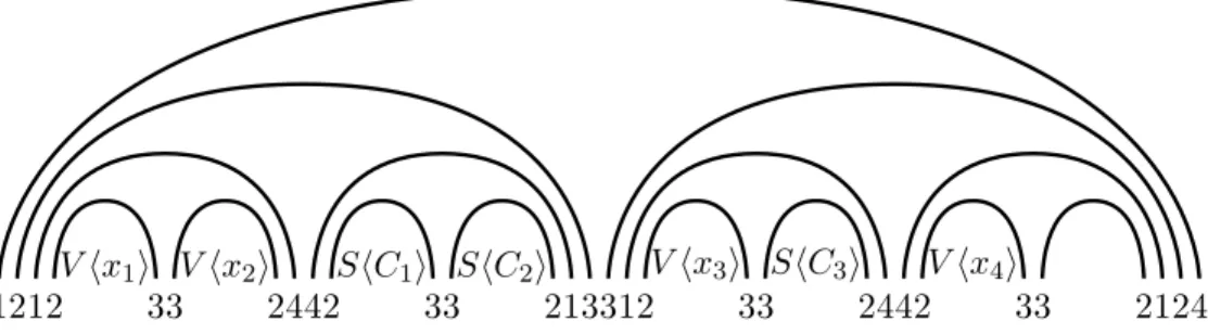
Overall construction. We join all the gadgets in a binary tree of Θ(n + m) = Θ(n) pairs of
parentheses and height Θ(log n) labeled such as illustrated in Figure 3. The only requirement on this labeling is that there is no other way of fully matching the binary tree onto itself. We say that a pair of matched parentheses is labeled by i-j (with i + j = 5) if the opening parenthesis is labeled by i (implying that the closing parenthesis has to be labeled by j = 5 − i). A possibility3
for labeling the binary tree is to use 1-4 for the outermost pair of parentheses and recursively use 2-3 and 3-2 for the two children of parentheses labeled by 1-4 or 4-1, and use 1-4 and 4-1 for the two children of parentheses labeled by 2-3 or 3-2. We denote by T the set of indices of the letters in this binary tree. At the “leaves” of the binary tree, we place the n + m variable and clause gadgets. The gadgets V hx1i, V hx2i, up to V hxni are placed from left to right. For i ∈ [n − 1], we reserve
some room in between V hxii and V hxi+1i for some clause gadgets, according to the following rule.
For each clause Cj on variables xa, xb, xc, with a < b < c, we insert the gadget ShCji somewhere
between V hxbiand V hxci; in other words, to the right of V hxbiand to the left of V hxci. Obviously,
such an ordering of the variable and clause gadgets can be found in polynomial time. The order of the clause gadgets that are between the same two consecutive variable gadgets V hxii and V hxi+1i
is not important and can be chosen arbitrarily. As n + m need not be a power of 2, there might be, as in Figure 3, some empty “leaves” without a variable gadget nor a clause gadget. We will show that the partial sequence w can be extended into a design for the structure S if and only if I is satisfiable.
The whole construction can be seen as simulating the following game, equivalent to 3-Sat, where your opponent has the more interesting role. There are boxes with 3 literals written on top of each box. At the beginning of the game, an opponent, who does not want you to get rich, chooses a truth assignment of the variables appearing on the boxes. Opening a box costs 2.99¤ of your favorite currency ¤. Once you open a box, you find inside one object per literal. You can turn this object into 1¤ if the literal is unsatisfied, and the object is worthless otherwise. You will decide to open a box only if its three literals are unsatisfied (and win 0.01¤). If you open a box with at least one satisfied literal, then you lose at least 0.99¤. If your opponent is computationally almighty, you will win nothing if and only if the formula is satisfiable.
In our case, opening a box by paying 2.99 ¤ corresponds to destroying, in a clause gadget, the q pairs of innermost parentheses surrounding the three literal gadgets (together with some Θ(log n) pairs of parentheses in T and an additional constant number within the clause gadget); and turning an object, found inside the box, associated to an unsatisfied literal `i into 1¤ corresponds to fully
pair the subtree V hxii to a subtree Lhxiior Lh¬xii.
3
Theorem 1 in [15] shows that there are exponentially many possible labelings for the tree. For more details, see the proof of Lemma 5 in the present paper.
V hx1i V hx2i ShC1i ShC2i V hx3i ShC3i V hx4i
1212 33 2442 33 213312 33 2442 33 2124
Figure 3: The overall picture with 4 variables and 3 clauses.
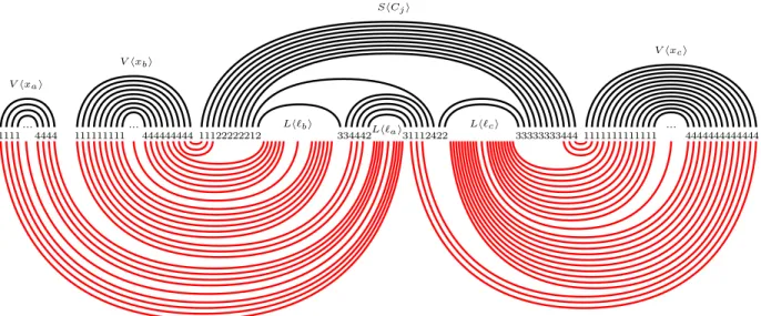
I unsatisfiable implies J has no design extension. Assume that instance I is not satisfiable.
By Lemma 4, we already observed that every potential solution corresponds to a truth assignment (via the interpretation: dots to 2 ≡ true, dots to 3 ≡ false). For any potential solution w0, let A
be the corresponding variable assignment. By assumption, there is a clause which is not satisfied by A; suppose it is the clause Cj = `a∨ `b∨ `c. We exhibit a structure S0 compatible with w0 and
with more paired letters than S (see Figure 4). The jy opening parentheses of the first layer of the arch of Cj are rematched to the last jy closing parentheses of the arch of xb, while the jy closing
parentheses of the first layer of the arch of Cj are rematched to the first jy opening parentheses of
the arch of xc. The letters whose indices are in A(q)j (second layer) become unpaired. We fully
rematch V hxbi, V hxai, and V hxci, to Lh`bi, Lh`ai, and Lh`ci, respectively. It is only possible since
all those three literals are unsatisfied by A; which means that, for any i ∈ {a, b, c}, if the dots in V hxiiare labeled by 2 (resp. 3), then the dots in Lh`iiare labeled by 3 (resp. 2). So, those dots can
be matched with each other. Observe that the extra arch above Lh`ai absorbs the jy first opening
parentheses of V hxbi and the last jy closing parentheses of V hxci.
Rematching those six sets of t consecutive dots incurs a win of 3t pairs. Let us now count the number of pairs in S that we lose. We have to break at most 6dlog(n + m)e pairs in T (indices in the binary tree), so that the six gadgets V hxai, V hxbi, V hxci, and Lh`ai, Lh`bi, Lh`ci in ShCji can
be rematched with each other. Those pairs that we break are all the parentheses in T in the paths going from those six gadgets to the root of the binary tree. Actually removing all the parentheses of T would still work. We also broke the q = 3t−10(n+m) pairs of indices in A(q), plus the 6 pairs of parentheses in ShCjiwhich are not part of an arch. The rest of S0 is matched as in S. This new
structure has at least 3t−(3t−10(n+m)+6)−6dlog(n+m)e = 10(n+m)−6(dlog(n+m)e+1) > 0 more pairs. Hence, S partially labeled by w cannot be extended into a design.
I satisfiable implies J has a design extension. Let A be a satisfiable assignment and let
w0 be the extension of w corresponding to A. We show that w0 is a design for S. For the sake of
contradiction, assume that there is a structure S06= S compatible with w0, having at least as many
pairs as S. Let us take S0 maximally matched.
Lemma 5. S0 has to match at least one letter which is unpaired in S.
Proof. Assume that S0does not match any unpaired letters in S. As S0has at least the same number
of paired letters as S, it implies that S0matches exactly the same letters (meaning the same indices)
as S. Let R0 (resp. R) be the structure obtained by restricting S0 (resp. S) to the paired letters
of S. Let ˆw be w0 restricted to those paired letters. By construction, R0 and R are two distinct
saturated structures both compatible with ˆw. In the proof of Theorem 1 in [15], the authors show
4 1 4 1 4 1 4 1 111111111 444444444111222222 3333334441111111111111 4444444444444 Lh`bi Lh` ai Lh`ci 12 334442 31112422 33 V hxai ... V hxbi ... V hxci ... ShCji
Figure 4: Suppose a clause Cj on variables xa, xb, and xc, with a < b < c, is not satisfied by the
extension w0. In red (light gray) is how we build a structure S0 with more pairs than S (in black).
this design can be found (in linear time) by a greedy labeling. The greedy labeling is any labeling which does not assign labels i-j to a child of paired parentheses labeled by j-i and avoids to label
two siblings with the same (oriented) pair i-j. Observe that R has degree at most 4 and that ˆw,
which we fully specified in the above construction, respects those two rules. Thus, ˆwis a design for R; a contradiction to the existence of R0.
The following lemma is straightforward and proves useful to argue about the quality of a struc-ture reachable from a partially built strucstruc-ture. It is based on a simple counting argument. For any i ∈ [4], we denote by #(i, w) the number of occurrences of i in the word w.
Lemma 6. If a structure contains (R) as a subtree (that is, the opening and closing parentheses
around R match) and the labeling ˆwof R is complete, then, for any i ∈ [4] and integer x, |#(i, ˆw) − #(5 − i, ˆw)| > x implies that more than x letters will remain unpaired.
Proof. Let ˆI be the set of (consecutive) indices of letters labeled by ˆw. Because of the surrounding parentheses, a base with index in ˆI has to be matched with a base with index also in ˆI. If, in ˆw, the number of i exceeds the number of 5 − i by more than x, then more than x bases i will not find a pairing 5 − i.
Let Di be the set of the dots contained in V hxii and in all the occurrences of Lh`ii (with
`i∈ {xi, ¬xi}).
Lemma 7. In S0, a base labeling a dot of Di can only be matched to a base labeling a dot of Di.
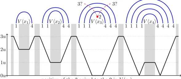
Proof. What is illustrated in Figure 5 is in fact more general, and extends from the variable gadgets
to the variable plus the literal gadgets. Suppose a base labeling a dot of Di is matched to a base
labeling a dot of Di0 with i 6= i0. Then, such a pair would surround a subsequence ˆw in w0 with
|#(1, ˆw) − #(4, ˆw)| > |i − i0|(m + 1)y > (m + 1)y = u > y, provided the two bases do not appear within the same clause gadget. If it is indeed the case, the inequality holds for the three subcases: variable-variable, variable-clause, and clause-clause (where X-Y says that the first base appears in an X gadget and the second base appears in a distinct Y gadget), and no matter which literal of the clause (first, second, or third) contains the base.
V hx1i 1 4 V hx2 i 1 1 4 4 V hx3 i 1 1 1 4 4 4 V hx4 i 1 1 1 1 4 4 4 4 2 3? 3? 0u 1u 2u 3u
position of the 3 paired to the 2 in V hx3i
Figure 5: Why pairing a letter in V hxii, not paired in S, to a letter in V hxi0iwith i 6= i0cannot give
a sufficiently paired structure. A single blue edge represents an arch of thickness u := (m+1)y. The y-axis corresponds to a lower bound of the imbalance |#(1, ˆw)−#(4, ˆw)|where ˆwis the subsequence surrounded by the new pair depicted by the red dashed edge. The gray areas mark positions where a 3 can actually be present. In those regions, |#(1, ˆw) − #(4, ˆw)| is greater than u, so this pairing necessarily yields a worse structure than S.
Now, if a base labeling a dot of Di in a literal gadget is matched to a base labeling a dot of Di0
in the same clause gadget ShCji (but a different literal gadget), then such a pair would surround a
subsequence ˆw in w0 with |#(1, ˆw) − #(4, ˆw)| > (|i − i0|(m + 1) − j)y > |m + 1 − j|y > y.
Finally, if a base labeling a dot of Di is matched to a base which is not labeling a dot of a Di0,
then the imbalance |#(1, ˆw) − #(4, ˆw)|, in the word ˆw surrounded by this pair, is larger, for some j ∈ [m], than (i(m + 1) − j)y > (m + 1 − m)y > y.
Recall that S has only y unpaired letters. By Lemma 6, in all those cases, S0 would have at
least y + 1 unpaired letters; a contradiction.
We will apply Lemma 6 again to argue that the second layer of the clause arches cannot be
significantly rematched. Let T0 be T augmented with the constant number per clause gadget of
indices corresponding to parentheses not in any arch.
Lemma 8. In S0, a letter with index in A(q)2j (resp. A(q)3j) can only be matched to a letter of T0∪ A(q)3
j (resp. T0∪ A(q)2j).
Proof. First, in S0, A(q)2
j cannot be rematched to A(q)3j0 with j 6= j0. Such a match would indeed
surround a subsequence ˆwin w0 with |#(1, ˆw) − #(4, ˆw)| > |j − j0|y. By Lemma 6 that would imply that S0 has strictly less pairs than S. Second, matching a letter with index in A(q)2
j to a 3 outside
of T0∪S
j0A(q)3j0 would mean to match it to a 3 labeling a dot in S. For this case, we can conclude
similarly to the proof of Lemma 7.
Let i ∈ [n] be such that a dot of Di labeled by 2 is matched in S0 to a dot of Di labeled by 3.
By Lemma 5 and Lemma 7, this index exists. Since Dicontains several literal gadgets but only one
variable gadget V hxii, at least one endpoint of this pair is in a clause gadget. Let j ∈ [m] be the
index of this clause. None of the pairs of parentheses of A(q)j can be present in S0; otherwise the
q pairs in S, have to be unpaired in S0; only a negligible O(n) of the corresponding letters could be rematched in T0.
Of the three literals of Cj, at most two are not satisfied by A. Let k ∈ [n] be the index of
a satisfied literal in Cj. The number of destroyed pairs of parentheses compared to S is at least
3t − O(n). At best, 2t new pairs are formed in S0 by linking literal gadgets in ShCji to the
corresponding variable gadgets. This still incurs a deficit of t − O(n) pairs. The dots in the literal
gadget of xk in ShCji have to be rematched. Otherwise, this contradicts the maximality of S0:
reversing locally S0 to S would provide a structure with strictly more pairs and would not create a
crossing.
By Lemma 7, the dots in the literal gadget of xk in ShCji can only be rematched to another
clause gadget ShCj0i containing the opposite literal of xk. By the same argument as for ShCji, this
rematching costs at least 3t − O(n) parentheses in A(q)j0 (so 6t − O(n) in total). And only 5t new
pairs can be obtained; this is the case if the four literals in the clauses Cj and Cj0 which are not on
the variable xk are unsatisfied and rematched to the corresponding variable gadgets4. The deficit
of this rematching is 6t − 5t − O(n) = t − O(n) > 0 (since we assumed that n, m are large enough). Thus reversing S0 to S locally would provide a structure with more pairs than S0, contradicting its
maximality.
4
Algorithmic results
In this section we show that the trivial O∗(4n)-time algorithm for the RNA Design problem can
be significantly improved by analyzing the tree representation of the input sequence.
Consider a structure S and its tree representation T . Let us define two families of subtrees that
can be found in T (we follow the notation used by Haleš et al. [16]). By m5 we denote a node of
degree more than 4. By m3◦ we denote a node with at least one unpaired child, and degree greater
than 2. We will use the following result by Haleš et al. [16] (note that both m5 and m3◦ do not
denote a specific subtree, but rather infinite families of subtrees).
Theorem 9 (Haleš et al. [16]). If S is designable, then it contains neither m5 nor m3◦.
Theorem 10. RNA Design Extension can be solved in time: (i) √3n· nO(1), where n is the length of the input structure,
(ii) 2s· nO(1), where s is the number of unlabeled elements in the input structure,
using polynomial space.
Proof. Let S be the input structure of length n and with s unlabeled elements. Let T be the tree representation of S and let r be the virtual root of T . By Theorem 9 we know that r has at most 4 children, each being either a matching pair of parentheses, or an unpaired letter. In the first step, we branch into all possible labelings of the unlabeled children of r. If there are no more unlabeled nodes, we check in polynomial time if the obtained labeling is a design of S, and if it extends the predefined partial labeling.
Consider a non-leaf node v of T , which is labeled, but all its children are unlabeled. Note that since v is not a leaf, it corresponds to a pair of matching parentheses.
We now want to branch into all possible labelings of children of r. However, in some cases we can prune the search tree, if we know that the current partial solution is not extendable to a design.
4Observe that this case is not even possible, since otherwise the clause C
j0 would not be satisfied by A, so the
By Theorem 9, we know that there are only very few possibilities of how the children of v look like. Either all of them are paired and then v has at most 3 children (otherwise we obtain m5), or v has
some unpaired children and at most one paired child (otherwise we obtain m3◦). Without loss of
generality assume that v is labeled with 1-4 (all other cases are symmetric).
11 42 32 34 14 12 33 24 ◦· · · ◦ ◦· · · ◦ 1 4 1 4 ◦...◦...◦ 1 1 4 ◦ ◦ ◦ ◦ 1 2 3 4
Figure 6: Some labelings which cannot be extended to a design, because they can be folded into some other structure with at least as many paired letters as in S (the first two pictures correspond to Case I, the third one to Case II, and the last two to Case III).
Case I. First, consider the case that v has d 6 3 children and all of them are paired. It is easy to verify that the only possible labelings of the children of v are: 1-4, 2-3, 3-2 (in any ordering, each of them may appear only once, see Figure 6 for some examples). This gives the recursion
F (n) 6 3!
(3 − d)!F (n − 2d),
where F (n) denotes the complexity of the discussed algorithm for the input structure of length n. The worst-case is achieved for d = 1 and has complexity F (n) = O∗(√3n) = O(1.7321n).
Case II.Now consider the case that v has one paired child and d > 1 unpaired ones. We observe
that the paired child of v can be labeled with 1-4 only, while the unpaired children can get either 2 or 3, but all of them must receive the same label (again, see Figure 6). This gives the recursion
F (n) 6 2F (n − 2 − d).
The worst case is achieved for d = 1 and has complexity F (n) = O∗(√3
2n) = O(1.2600n).
Case III.Finally, consider the case that v has d > 1 unpaired children and no paired ones. Let us call such a node bad. We observe that all children of v must receive the same label, either 2 or 3 (again, see Figure 6), thus the recursion for this case is
F (n) 6 2F (n − d),
which gives the complexity bound F (n) = O∗(2n)(achieved for d = 1).
However, we can show that this case cannot happen too often. We say that a node of T ,
which has at least two paired children, is good. Let T0 be a tree constructed from T by removing
all unpaired nodes, and contracting all induced paths into single edges (thus we remove nodes of
degree 2). Moreover, if the virtual root r of T has degree 1, we remove it and assume that T0 is
rooted at the only child of r. It is easy to observe that T0 has the following properties:
(a) every node of T0 is also a node of T ,
(b) the root of T0 has at most 4 children,
(c) every inner node of T0 has 2 or 3 children,
(e) every bad vertex of T is a leaf of T0.
Let z be the number of leaves in T0, clearly the number of bad vertices in T is at most z. Since
every inner node of T0 has at most 3 children, we observe that the number of inner nodes in T0 is at
least (z − 4)/2, so this gives us a lower bound for the number of good nodes in T . Thus, for every two bad nodes (up to a constant number exceptional ones), there exists a good node (which is not shared with any other pair of bad nodes). More formally speaking, we can partition the set of all but a constant number of bad nodes into a family A of two-elements sets, and define an injective mapping from A to the set of good nodes of T . So, if we consider labeling children of two bad nodes
(with d1 and d2 unpaired children, respectively) and d > 2 children of a good node at the same
time, we obtain the recursion
F (n) 6 22· 6 · F (n − d1− d2− 2d).
The worst case-complexity for this case is achieved for d1 = d2 = 1 and d = 2, which gives us
F (n) 6 24F (n − 1 − 1 − 4) = 24F (n − 6), so F (n) = O∗(√624n) = O(1.6984n). Since there is only a constant number of bad nodes which are not paired with good nodes, the blow-up in complexity is also a constant and can be ignored in O(·)-notation.
The correctness of the described procedure is clear and follows from the fact that we only discard labeling which cannot appear in any design. The running time of the procedure is determined by the complexity of the worst-case branching, which appears in Case I for d = 1, and thus the running time can be bounded by F (n) = O∗(√3n) = O(1.7321n).
Note that the above recursive procedure is completely oblivious to the initial partial labeling of
S. The only place where we make use of it is the final checking. In our second approach we will
only construct partial labelings which extend the pre-labeling.
First, observe that if S has a matching pair and one of its elements is already labeled, the label of the other element is also uniquely determined. Thus we can assume that each node of T is either labeled (i.e., if it is a paired node, then both parentheses are already labeled), or unlabeled.
The cases we consider are the same as in the first algorithm, but now the size of the problem is s, the number of unlabeled elements in the input structure.
Case I.Let d be the number of paired children of v, p of which are unlabeled. We have 1 6 p 6 d 6
3. Considering all cases, we observe that the worst case is achieved for d = p = 1. It is described by the recursion
F0(s) 6 3F0(s − 2),
and its complexity is F0(s) =√3s· nO(1),where F0(s) is the complexity of the discussed algorithm
for an input structure with s unlabeled elements.
Case II. Recall that the labeling of the paired child of v must be the same as the labeling of v.
Thus, without loss of generality, we can assume that the paired child of v is labeled. Also, if at least one of unpaired children is labeled, we can extend the labeling to all other unlabeled children. Suppose that v has d > 1 unpaired children We obtain the recursion
F0(s) 6 2F0(s − d).
Its worst-case is achieved for d = 1, and the complexity is F0(s) = 2s· nO(1).
Case III. This case is analogous to the previous one – all d unpaired children of v get the same
label. The recursion for this case is
F0(s) 6 2F0(s − d),
The correctness is straightforward and the complexity bound for the whole procedure is F0(s) =
2s· nO(1).
Finally, let us remark that Haleš et al. [16] give a complete characterization of saturated struc-tures (i.e., ones without unpaired elements), which have a design. This characterization implies a polynomial-time algorithm for the RNA design problem on such structures. Using bottom-up dy-namic programming on the tree representation on the input structure, we can adapt this procedure to the more general RNA Design Extension problem.
Observation 11. RNA Design Extension is tractable on saturated structures.
References
[1] R. Aguirre-Hernández, H. H. Hoos, and A. Condon. Computational RNA secondary structure design: empirical complexity and improved methods. BMC Bioinformatics, 8(1):34, 2007. [2] T. Akutsu. Dynamic programming algorithms for RNA secondary structure prediction with
pseudoknots. Discrete Applied Mathematics, 104(1):45–62, 2000.
[3] J. Anderson-Lee, E. Fisker, V. Kosaraju, M. Wu, J. Kong, J. Lee, M. Lee, M. Zada, A. Treuille, and R. Das. Principles for predicting RNA secondary structure design difficulty. Journal of Molecular Biology, 428(5, Part A):748 – 757, 2016.
[4] M. Andronescu, A. P. Fejes, F. Hutter, H. H. Hoos, and A. Condon. A New Algorithm for RNA Secondary Structure Design. Journal of Molecular Biology, 336(3):607 – 624, 2004. [5] C. Anfinsen. Principles that govern the folding of protein chains. Science, 181(4096):223, 1973. [6] M. Biró, M. Hujter, and Z. Tuza. Precoloring extension. I. Interval graphs. Discrete
Mathe-matics, 100(1-3):267–279, 1992.
[7] A. E. Borujeni, D. M. Mishler, J. Wang, W. Huso, and H. M. Salis. Automated physics-based design of synthetic riboswitches from diverse RNA aptamers. Nucleic Acids Research, 44(1):1–13, 2016.
[8] K. Bringmann, F. Grandoni, B. Saha, and V. V. Williams. Truly Sub-cubic Algorithms for Language Edit Distance and RNA-Folding via Fast Bounded-Difference Min-Plus Product. In I. Dinur, editor, IEEE 57th Annual Symposium on Foundations of Computer Science, FOCS 2016, pages 375–384. IEEE Computer Society, 2016.
[9] G. L. Butterfoss and B. Kuhlman. Computer-based design of novel protein structures. Annual review of biophysics and biomolecular structure, 35:49–65, 2006.
[10] H. Chen, A. Condon, and H. Jabbari. An O(n5) Algorithm for MFE Prediction of Kissing Hairpins and 4-Chains in Nucleic Acids. Journal of Computational Biology, 16(6):803–815, 2009.
[11] A. Churkin, M. D. Retwitzer, V. Reinharz, Y. Ponty, J. Waldispühl, and D. Barash. Design of RNAs: Comparing Programs for inverse RNA folding. Briefings in Bioinformatics, 2017.
[12] A. Condon. Problems on RNA Secondary Structure Prediction and Design. In J. C. M. Baeten, J. K. Lenstra, J. Parrow, and G. J. Woeginger, editors, Automata, Languages and Programming, 30th International Colloquium, ICALP 2003, volume 2719 of LNCS, pages 22– 32. Springer, 2003.
[13] A. Condon. RNA Molecules: Glimpses Through an Algorithmic Lens. In J. R. Correa, A. Hevia, and M. A. Kiwi, editors, Proceedings of LATIN 2006: Theoretical Informatics, 7th Latin Amer-ican Symposium, volume 3887 of LNCS, pages 8–10. Springer, 2006.
[14] J. A. García-Martín, P. Clote, and I. Dotú. RNAiFold: a web server for RNA inverse folding and molecular design. Nucleic Acids Research, 41(Webserver-Issue):465–470, 2013.
[15] J. Haleš, A. Héliou, J. Maňuch, Y. Ponty, and L. Stacho. Combinatorial RNA Design: Des-ignability and Structure-Approximating Algorithm. In F. Cicalese, E. Porat, and U. Vaccaro, editors, Combinatorial Pattern Matching - 26th Annual Symposium, CPM 2015, Proceedings, volume 9133 of LNCS, pages 231–246. Springer, 2015.
[16] J. Haleš, A. Héliou, J. Maňuch, Y. Ponty, and L. Stacho. Combinatorial RNA Design: Des-ignability and Structure-Approximating Algorithm in Watson-Crick and Nussinov-Jacobson Energy Models. Algorithmica, 2016. To appear.
[17] I. Hofacker, W. Fontana, P. Stadler, L. Bonhoeffer, and M. Tacker. Fast Folding and Compari-son of RNA Secondary Structures. Monatshefte für Chemie (Chemical Monthly), 125:167–188, 1994.
[18] S. Ieong, M.-Y. Kao, T.-W. Lam, W.-K. Sung, and S.-M. Yiu. Predicting RNA secondary structures with arbitrary pseudoknots by maximizing the number of stacking pairs. Journal of Computational biology, 10(6):981–995, 2003.
[19] H. Jabbari, A. Condon, and S. Zhao. Novel and efficient RNA secondary structure prediction using hierarchical folding. Journal of Computational Biology, 15(2):139–163, 2008.
[20] J. Lee, W. Kladwang, M. Lee, D. Cantu, M. Azizyan, H. Kim, A. Limpaecher, S. Gaikwad, S. Yoon, A. Treuille, R. Das, and EteRNA Participants. RNA design rules from a massive open laboratory. Proceedings of the National Academy of Sciences, 111(6):2122–2127, 2014.
[21] R. B. Lyngsø. Inverse folding of RNA. http://citeseerx.ist.psu.edu/viewdoc/download? doi=10.1.1.226.5439&rep=rep1&type=pdf.
[22] R. B. Lyngsø. Complexity of Pseudoknot Prediction in Simple Models. In Automata, Languages and Programming: 31st International Colloquium, ICALP 2004, Turku, Finland, July 12-16, 2004. Proceedings, pages 919–931, 2004.
[23] R. B. Lyngsø and C. N. S. Pedersen. RNA Pseudoknot Prediction in Energy-Based Models. Journal of Computational Biology, 7(3-4):409–427, 2000.
[24] R. Nussinov and A. B. Jacobson. Fast algorithm for predicting the secondary structure of single-stranded RNA. Proceedings of the National Academy of Sciences, 77(11):6309–6313, 1980.
[25] E. Rivas and S. R. Eddy. A dynamic programming algorithm for RNA structure prediction including pseudoknots. Journal of molecular biology, 285(5):2053–2068, 1999.
[26] G. Rodrigo, T. E. Landrain, and A. Jaramillo. De novo automated design of small RNA circuits for engineering synthetic riboregulation in living cells. Proceedings of the National Academy of Sciences, 109(38):15271–15276, 2012.
[27] B. Saha. Fast & Space-Efficient Approximations of Language Edit Distance and RNA-Folding: An Amnesic Dynamic Programming Approach. In IEEE 58th Annual Symposium on Founda-tions of Computer Science, FOCS 2017. To appear.
[28] M. Schnall-Levin, L. Chindelevitch, and B. Berger. Inverting the Viterbi algorithm: an abstract framework for structure design. In W. W. Cohen, A. McCallum, and S. T. Roweis, editors, Machine Learning, Proceedings of the Twenty-Fifth International Conference (ICML 2008), volume 307 of ACM International Conference Proceeding Series, pages 904–911. ACM, 2008. [29] J. E. Tabaska, R. B. Cary, H. N. Gabow, and G. D. Stormo. An RNA folding method capable
of identifying pseudoknots and base triples. Bioinformatics (Oxford, England), 14(8):691–699, 1998.
[30] C. A. Tovey. A simplified NP-complete satisfiability problem. Discrete Applied Mathematics, 8(1):85–89, 1984.
[31] Y. Zhou, Y. Ponty, S. Vialette, J. Waldispühl, Y. Zhang, and A. Denise. Flexible RNA design under structure and sequence constraints using formal languages. In J. Gao, editor, ACM Conference on Bioinformatics, Computational Biology and Biomedical Informatics. ACM-BCB 2013, page 229. ACM, 2013.
[32] M. Zuker and P. Stiegler. Optimal computer folding of large RNA sequences using thermody-namics and auxiliary information. Nucleic acids research, 9(1):133–148, 1981.