Multicriteria assignment of tasks to heterogeneous processing units with incomparability and capacity constraints

MULTI-CRITERIA ASSIGNMENT OF TASKS

TO HETEROGENEOUS PROCESSING UNITS

WITH INCOMPATIBILITY AND CAPACITY

CONSTRAINTS

Bernard Roy

1

_{, Roman Słowiński}

2

1_{LAMSADE, University of Paris Dauphine, 75775 Paris, France;} roy@lamsade.dauphine.fr

2_{Institute of Computing Science, Poznań University of Technology,} 60-965 Poznań, Poland; slowinsk@sol.put.poznan.pl

1. Introduction and problem statement

We are considering the following assignment problem. A finite set T of tasks th, h=1,...,n, has to

be assigned to a finite set P of processing units pj, j=1,...,m. Each task th has to be assigned to

exactly one processing unit, however, more than one processing unit is able to process th. Each

task th has, moreover, a different “preference” for being assigned to a particular processing unit;

this “preference” is expressed by a dissatisfaction degree of th for being assigned to pj, denoted

by dhj. The dissatisfaction degree dhj≥0 for h=1,...,n; j=1,...,m; the greater dhj the higher the

dissatisfaction; dhj=∞ means impossibility of assigning th to processing unit pj.

Each processing unit pj has a regular capacity of processing mj tasks. This capacity is flexible to

some extent and can be increased up to Mj≥mj tasks, however, only mj tasks can be processed on

pj without any cost. One additional task over mj augments the processing cost of pj by a marginal

cost c_j1>0, similarly, the second additional task byc_j2, etc., until the (Mj-mj)-th additional task

that augments the processing cost by , where these marginal costs are non-decreasing.

Obviously, . ) (Mj mj j c ₋ n M m j j ≥

∑

=1

The assignment of tasks to processing units has to respect some incompatibility constraints. Let

⊆T, i=1,...,u

ij

Q j, j=1,...,m, be a subset of tasks such that each th∈ can be processed by

processing unit p

ij

Q

ij

Q

j, however, in a feasible assignment, at most one th∈ can be assigned to pj,

for i=1,...,uj and j=1,...,m. Qij is called the i-th incompatibility group of processing unit pj.

Different incompatibility groups of the same processing unit must be disjoint. If a task th can be

processed by a processing unit pj and if th∉Qij, i=1,...,u

ij

Q

j, then pj is said to be able to process th

directly; if th belongs to one of incompatibility groups of pj, then pj is said to be able to process th

indirectly. It follows from the definition of that a task th which can be processed directly by a

processing unit pj does not enter any incompatibility group of pj.

The quality of feasible assignments is evaluated by three criteria: G1 - the maximum

dissatisfaction of tasks, G2 - the total dissatisfaction of tasks, G3 - the total cost of processing

units.

One can meet assignment problems of this type in many real life situations. Let us give a few examples:

a). Organization of the students’ choice of optional courses1

Each processing unit corresponds here to a course (or seminar) that students may have to follow in order to obtain a diploma. Each student ei has to follow a fixed number u of courses chosen

from among set P of courses given by different professors. Student ei is thus associated with u

tasks: ti1,…,tiu.

For each task ti1,…,tiu, student ei presents two possibilities: the first possibility points out a first

choice course (dissatisfaction zero) while the other, a second choice course (dissatisfaction greater than zero). All u first choices must be different. As to second choices, they do not need to

be different neither among them nor from the first choices. It is thus possible that a course pj is

pointed out many times by student ei in the secondary choice and also once in the first choice

(some reasonable constraints impose a minimum diversity). Let Qij be a set of tasks for which

student ei has pointed out course pj; as this course may be followed only once, Qij is the i-th

incompatibility group of processing unit pj; in this case, pj can process indirectly each task

included in Qij. If student ei has pointed out course pj only once, then the corresponding task can

be processed directly by pj.

The way in which some courses are organized (students’ oral reports or limited access to some facilities) can lead to fixing an upper bound on the number of students accepted for the course. It is then realistic to represent this constraint by two limits: the first one, that would be desirable to keep (regular capacity mj), and the second one, that is rather impossible to overstep (maximal

capacity Mj). Each additional student over mj deteriorates the conditions in which the course is

carried out, and the deterioration rate increases with the number of additional students. b). Timetabling

One is considering here a set of activities (courses, exams, meetings, exhibitions, etc.) that should be scheduled over time. These activities should be performed in places called rooms. Moreover, they have the same unit duration that fits a time slot. For a given activity th, many

time slots are possible but they are more or less satisfactory. During each time slot pj, mj rooms

are normally available, but it is also possible to adapt some extra rooms at additional cost depending on the room.

1 _{A problem of this type arises when students (preparing a diploma in scientific methods of management at}

the University of Paris Dauphine) are to be assigned to one major and one minor seminar, taking into account their preferences and pedagogic capacity of professors. The case of Dauphine students was at the origin of the present study, however, before the present model was set up, a less general one existed together with preliminary software made in collaboration with several students. B. Roy used this supporting tool during the last decade, as a director of this diploma.

In this case, the tasks represent activities, and the processing units – time slots with available rooms. The incompatibility groups of time slot pj are composed of activities that can be

performed in this time slot but assignment of one activity to that slot excludes assignment of any other from this group, as they all require the same resource, for example a professor, a facility or the same group of participants.

c). Scheduling on machines

Set T of n tasks has to be processed on set P of m parallel heterogeneous machines (e.g.

processors of a parallel computer system). The processing of each task on a particular machine is more or less efficient (dissatisfaction degree) and some tasks, in addition to a machine, require a unique additional resource (e.g. input-output channel, printer etc.). Each machine pj is normally

available in mj copies which can be enlarged to Mj at some extra cost (e.g. spent for

communication). The incompatibility groups of a given machine are composed of tasks that can be processed on this machine and require the same additional resource.

Many other applications can fit the considered model, in particular, from the field of personnel management, distribution and transportation. In all these contexts two types of questions arise:

i). If all tasks from set T can be assigned, how to define and choose the “best assignment”?

An assignment that accepts some dissatisfaction of tasks will be, in general, more economic than an assignment which tends to perform each task in most satisfactory conditions. The latter may introduce indeed high costs of overloading some processing units. In consequence, it seems reasonable to search for a compromise between dissatisfaction of tasks (maximum dissatisfaction degree and total dissatisfaction) and the cost of overloading the processing units.

ii). If it is impossible to assign all tasks from set T, how to characterize the reasons of this

impossibility? After they have been clearly identified, what actions can be undertaken (modifications of some input data) to enable additional assignments?

The paper is aiming at answering the above questions. It is organized in the following way. In section 2, the problem of finding a feasible assignment is formulated as a problem of finding a maximum integer flow in a special network. Section 3 is devoted to analysis of the case of impossible assignment; subsets of tasks, incompatibility groups and processing units that are responsible for this impossibility constitute so-called blocking configuration; to solve the impossibility problem, six actions of unblocking are identified; it is then demonstrated that they are the only ones which can create possibilities of additional assignments. The multi-criteria

assignment problem is considered in section 4; a strategy for selection of the best compromise assignment with respect to the three criteria G1, G2, G3 defined above is outlined. Section 5

presents procedures for exploration of a set of non-dominated assignments on the plane (G2×G3);

they are specialized in searching for supported and non-supported solutions, respectively. Numerical examples with and without blocking configuration are presented in section 6; they are solved using a specialized software called MASCOME (Multi-criteria Assignment Subject to Constraints Of Mutual Exclusion) (Slowinski, 2001). Conclusions are drawn in section 7.

2. Modeling the set of feasible assignments

The problem of finding a feasible assignment of tasks from T to processing units from P can be

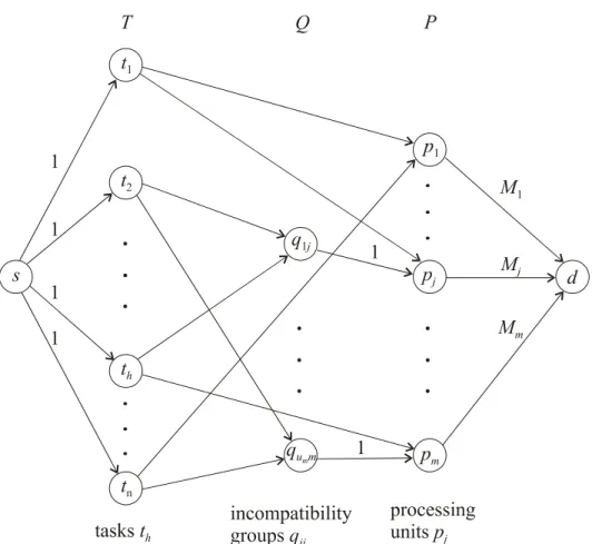
formulated as a problem of finding a maximum integer flow in the network N, shown in Fig. 1, being characterized by:

a set of vertices V in which two special vertices are distinguished: a source s and destination d, 1)

2) 3)

a set of directed arcs W ⊆ V × V,

integer numbers κ(w)≥0, associated with each arc w∈W, called the capacity of arc w, giving the upper bound for the flow on this arc; the lower bound on all arc flows is equal to zero. Specifically, apart from s and d, the vertex set V is composed of three subsets:

• T, including n vertices th corresponding to the tasks (h=1,..,n),

• Q, including u vertices qij corresponding to incompatibility groups Qij (i=1,...,uj, j=1,...,m;

u=

∑

m_j=1u_j ),

• P, including m vertices pj corresponding to the processing units (j=1,...,m).

Below, when speaking about incompatibility groups in the network context, we will use the vertex notation qij instead of the set notation . The arc set W is composed of five types of

arcs:

ij

Q

• arcs (s, th), called entering arcs, with capacity equal to one,

• arcs (th, pj), called directly connecting arcs, with unlimited capacity,

• arcs (th, qij), called indirectly connecting arcs, with unlimited capacity,

• arcs (qij, pj), called incompatibility arcs, with capacity equal to one,

The network N has n entering arcs, m leaving arcs and u incompatibility arcs. Moreover, the

directly connecting arc (th, pj) exists in N if and only if task th can be processed directly by

processing unit pj. Finally, the indirectly connecting arc (th, qij) exists in N if and only if

processing unit pj can process task th indirectly, that is if th belongs to the i-th incompatibility

group of pj. Thus, there is at most one path from th to pj.

Fig. 1. Finding a feasible assignment as a problem of finding a maximum integer flow in network N

Obviously, every integer flow in the network N, having value equal to n, represents an

assignment respecting the constraints of our problem and, vice versa, for any assignment respecting the constraints of our problem, one can find an integer flow equal to n in the network

N. Clearly, each flow in N equal to n is a maximum flow in N, but the converse is not true.

If a maximum flow in N does not saturate all entering arcs, that is if the value of the maximum flow is n-ρ, and ρ>0, then this means that it is impossible to assign ρ tasks to available

processing units, given the imposed constraints. In section 3, we will show that this impossibility comes from an existence in N of a configuration of tasks, processing units and incompatibility

groups called blocking configuration. We will then analyze blocking configurations in order to

formulate all possible relaxations of the constraints enabling a complete assignment.

3. Analysis of blocking configurations and actions of unblocking 3.1. A brief reminder of network flow properties

Let us consider a maximum flow in network N and the associated labeling procedure defined as follows:

vertex s is labeled, 1)

2) 3)

any vertex following a labeled vertex via a non-saturated arc is also labeled, any vertex preceding a labeled vertex via a non-empty arc is also labeled.

According to the well-known maximum-flow minimum-cut theorem of Ford and Fulkerson (1962), we know that:

• the flow in a network has a maximum value if and only if vertex d is unlabeled,

• if vertex d has been labeled then the labels give a hint how to augment the flow in the network.

The theorem of Ford and Fulkerson states, moreover, that the value of the maximum flow from s

to d is equal to the value of a minimum cut-set separating s from d. Such a cut-set is revealed by

the labeling procedure: it is composed of all the arcs whose initial vertices are labeled and final vertices are unlabeled; the sum of the capacities of these arcs defines what is called the capacity of the cut-set. The arcs of the cut-set are necessarily saturated and each path connecting s and d

necessarily includes one arc from the cut-set.

3.2. Analysis of the minimum cut-set of network N

Given a maximum flow, the minimum cut-set of network N, revealed by the Ford-Fulkerson labeling procedure, contains the following arcs:

(i) entering arcs whose final vertices are unlabeled – their total capacity is equal to x,

(ii) incompatibility arcs whose initial vertices are labeled and final vertices are unlabeled – their total capacity is equal to z; the initial vertices of these saturated arcs are called saturated incompatibility groups,

(iii) leaving arcs whose initial vertices are labeled – their total capacity is equal to µ; the initial vertices of these saturated arcs are called saturated processing units.

Observe that there are no directly nor indirectly connecting arcs in the minimum cut-set since they have an unlimited capacity.

The total capacity of saturated arcs (i), (ii) and (iii) is equal to x+z+µ. Thus, according to the theorem of Ford and Fulkerson,

x + z + µ = n - ρ. (3.1)

The number of tasks that it is impossible to assign, given the imposed constraints, is equal to

ρ = n - x - z - µ.

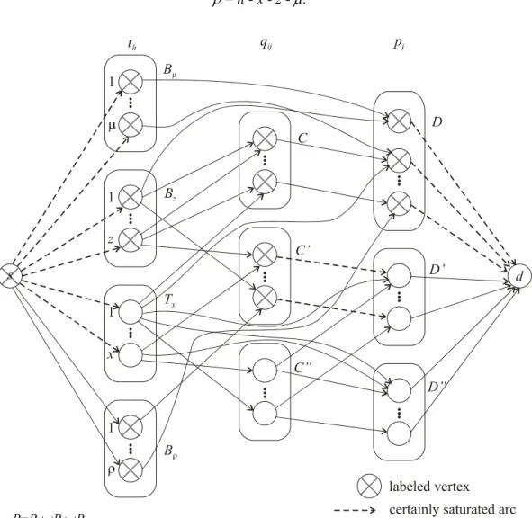
Fig. 2. Example of partition of sets T, Q, P

To understand why the flow cannot be greater than n - ρ, it is useful to introduce the following notation.

One can distinguish the following subsets of tasks in the set T:

Tx – set of x unlabeled tasks th (final vertices of arcs (i) in the minimum cut-set),

Bz – set of z tasks th processed via z saturated incompatibility groups (initial vertices of arcs (ii)

in the minimum cut-set),

Bµ – set of µ tasks th processed by saturated processing units (initial vertices of arcs (iii) in the

minimum cut-set),

Bρ – set of ρ non-assigned tasks th,

B = Bz∪Bµ∪Bρ – set of labeled tasks.

It follows from (3.1) that Tx, Bz, Bµ and Bρ are four disjoint sets. Therefore, Bz, Bµ, Bρ is a

partition of B.

The set Q of incompatibility groups can be partitioned into the following subsets: C – set of labeled incompatibility groups qij connected to labeled processing units pj,

C’ – set of z labeled incompatibility groups qij connected to unlabeled processing units pj

(saturated incompatibility groups being initial vertices of arcs (ii) in the minimum cut-set),

C’’ – set of unlabeled incompatibility groups qij.

The set P of processing units can be partitioned into the following subsets (see Fig. 2): D – set of labeled processing units pj with total capacity of outgoing arcs equal to µ (saturated

processing units being initial vertices of arcs (iii) in the minimum cut-set),

D’ – set of unlabeled processing units pj having at least one predecessor in C’; observe that

card(D’)≤ z, and pj∈D’ can also have some predecessors in C’’ and in Tx, but not in B or in

C, because otherwise it would be labeled,

D’’ – set of unlabeled processing units pj having all their predecessors in C’’ or in Tx.

3.3. The concept of the blocking configuration

Definition 1: The triplet <B, C’, D> revealed by the Ford-Fulkerson labeling procedure,

associated with a maximum flow in N, is called a blocking configuration.

Theorem 1: Consider a maximum flow in N and the associated blocking configuration

<B, C’, D>. The following statements are true:

1. From among the n-x tasks of B, µ tasks can be processed by saturated processing units pj∈D,

and z other tasks by processing units pj∉D via z saturated incompatibility groups qij∈C’. No

other processing unit pj can process any of the n-x tasks. Thus, the maximum number of tasks

th∈B that can be assigned to processing units from P is equal to

+ card(C’) = z + µ.

∑

j∈{j:p_j∈D}Mj

2. The blocking configuration <B, C’, D> is independent of the maximum flow used to reveal

this configuration.

Proof of statement 1: No processing unit pj∈D’’ is adjacent to a task th∈B because, otherwise, it

would be labeled. For the same reason, no incompatibility group qij∈C’’ of a processing unit

pj∈D’’ is adjacent to a task th∈B. Thus, no processing unit pj∈D’’ can process directly nor

indirectly a task th∈B, so the only processing units that could do it are in D and D’. Moreover, for

the same reason as above, a processing unit pj∈D’ is not adjacent to a task th∈B. If a processing

unit pj∈D’ is adjacent to an incompatibility group qij∈C’’, then this group is not adjacent to a

task th∈B because, otherwise, it would be labeled. Thus, the processing unit pj∈D’ can process a

task th∈B only indirectly via an incompatibility group qij∈C’. As there are z incompatibility

groups in C’, the processing units pj∈D’ cannot process more than z tasks th∈B, whatever their

total capacity. The total capacity of processing units pj∈D is limited by = µ

because all the leaving arcs outgoing p

∑

j∈{j:p_j∈D}Mj j∈D are saturated. Consequently, the processing units from

P can process at most z+µ tasks th∈B. This can be done exclusively by the processing units pj∈D

or by those processing units which have an incompatibility group in C’.

Proof of statement 2: Let us start by proving2 the following lemma.

Lemma: The set of vertices labeled by the procedure of Ford and Fulkerson is independent of

the maximum flow that is used to perform this labeling.

Proof of the lemma: Each subset of vertices M⊂V, such that s∈M and d∉M, defines a cut-set

Ω(M) composed of arcs (x,y) such that x∈M and y∉M. Let K[Ω(M)] denote the capacity of this

cut-set.

2 _{This result has possibly been proved already, however, we did not find any trace of that in classic books.}

We wish to thank Daniel Vanderpooten who gave us the basis of the following demonstration, shorter and more elegant than the one we have initially made.

Let us consider two distinct maximum flows Φ1 and Φ2. Let also M1 denote the set of vertices

labeled with Φ1, and M2, the set of vertices labeled with Φ2. Being maximum, these flows have

the same capacity equal to m, so that:

m = K[Ω(M1)] = K[Ω(M2)]. (3.2)

Fig. 3. Graphical support for the proof of the lemma

The subsets M1∩M2 and M1∪M2 include s but not d. Thus, their associated cut-sets verify:

K[Ω(M1∩M2)] ≥ m, K[Ω(M1∪M2)] ≥ m. (3.3)

Let M’1= M1\M2 and M’2= M2\M1. Using these subsets one can define the two following subsets

of arcs:

Y, the set of arcs (x,y) such that x∈ M’1, y∈M’2, Z, the set of arcs (y,x) such that y∈M’2, x∈M’1.

It is sufficient to analyze the subsets of arcs belonging to the cut-sets Ω(M1), Ω(M2), Ω(M1∩M2),

Ω(M1∪M2) (see Fig. 3) to verify that:

K[Ω(M1)] + K[Ω(M2)] = K[Ω(M1∩M2)] + K[Ω(M1∪M2)] + K(Y) + K(Z)

K[Ω(M1)] + K[Ω(M2)] ≥ K[Ω(M1∩M2)] + K[Ω(M1∪M2)]. (3.4)

It follows from (3.2), (3.3) and (3.4) that:

K[Ω(M1∩M2)] = K[Ω(M1∪M2)] = m.

Ω(M1∩M2) is thus a minimum cut-set. In consequence, independently of the flow considered (Φ1

or Φ2), once the vertices M1∩M2 are labeled, any other vertex cannot be labeled. We have thus M1 = M2.

The lemma being proved, one can derive immediately that set B of labeled tasks does not depend

on the maximum flow considered. It is so for the set D of labeled processing units and for the set C∪C’ of labeled incompatibility groups. A labeled incompatibility group is in C’ if and only if its unique successor in D’ is not labeled. This is also independent of the maximum flow

considered. This ends the proof of statement 2.

Corollary:

1). The partition [C, C’, C’’] of incompatibility groups and the partition [D, D’, D’’] of

processing units do not depend on the maximum flow considered.

2). The x tasks not belonging to B are assigned to processing units in each maximum flow;

they can only be processed by processing units from D’∪D’’; if a processing unit pj∈D’

is able to process one of these tasks, then this task can be assigned to pj only directly or

indirectly through incompatibility group qij∈C’’ such that Qij∈Tx.

3). The processing units from D∪D’ are the only ones that can process the tasks from set B; if a processing unit pj∈D’ is able to process one of these tasks, then this task can be

assigned to pj only indirectly through incompatibility group qij such that Qij⊂B;

moreover, in each maximum flow, one task of each such incompatibility group is assigned to the processing unit pj∈D’; this means that this processing unit cannot

process more tasks from B.

4). The partition [Bµ, Bz, Bρ] of B is not independent of the maximum flow considered.

Proof of the corollary:

1). This result follows immediately from the second statement of the theorem.

2). Whatever the maximum flow considered, the only tasks being labeled are in B, thus the

tasks from Tx cannot be labeled. Let th∈Tx. The arc (s, th) is necessarily saturated because

processing unit is certainly not from set D because pj∈D are labeled, so th would also be

labeled. Thus, only the processing units from D’∪D’’ are able to process th. Consider

any processing unit pj∈D’; since this processing unit is unlabeled, it can process th

directly. Now, consider an incompatibility group Qij represented by vertex qij ; if qij is

labeled (qij∈C’), then th∉Qij. As soon as Qij contains at least one task from B, qij is

labeled. Thus, if th∈Qij, then Qij∈Tx.

3). If pj∈D’’ would be able to process directly a task from set B, then pj would be labeled

because all tasks from B are labeled. If pj would be able to process indirectly a task from

set B, then the corresponding incompatibility group would be labeled. pj∈D’’ has,

however, no predecessor among labeled incompatibility groups. For the same reason,

pj∈D’ cannot process directly any task from set B. If it is able to process one task from B

through incompatibility group qij, then one task of this incompatibility group is

necessarily assigned to pj because, qij being labeled and pj being not, the arc (qij, pj) is

saturated. Thus, pj∈D’ is processing a number of tasks from B equal to the number of all

its incompatibility groups qij, i=1,…,uj. In any flow, it cannot process more.

4). The following example is sufficient to show that the partition [Bµ, Bz, Bρ] of B is not

independent of the maximum flow considered. Let T={t1, t2, t3} and P={p1, p2} such that: t1 can only be processed by p1 directly,

t2 can be processed by p1 directly and by p2 indirectly, because of the 2-incompatibility

group Q12={t2, t3},

t3 can only be processed by p2 indirectly, because of the 2-incompatibility group Q12, p1 and p2 can process one task each.

Consider two maximum flows presented in Fig. 4, giving the following assignments: a) t1 is assigned to p1 and t2 is assigned to p2 through incompatibility group q12, which

results in

Bµ={t1}, Bz={t2}, Bρ={t3},

b) t2 is assigned to p1 and t3 is assigned to p2 through incompatibility group q12, which

results in

The example presented in point 6.1 illustrates all properties connected with the concept of a blocking configuration.

Fig. 4. For alternative maximum flows, the labeling does not change but Bµ, B z andBρ do

change

3.4. Actions of unblocking

What action should be made in order to relax the imposed constraints such that one of the tasks

We suppose that the only possible modifications of initial data aiming at processing one additional task are of the following types:

1° Augment the capacity of a processing unit pj.

2° Allow a processing unit pj to process directly a task th that it was unable to process, neither

directly nor indirectly.

3° Allow a processing unit pj to process indirectly a task th that it was unable to process, neither

directly nor indirectly, putting th in one of incompatibility groups of pj.

4° Allow a processing unit pj to process directly a task th that it was able to process indirectly

only.

It follows that any action able to unblock the impossibility of assigning one additional task, consists in making one or more modifications of the above types. The modifications 2°, 3°, 4° are mutually exclusive, however, each of them can be combined with the first modification. In order to augment the assignment of tasks to processing units, one has to consider these modifications with respect to each maximum flow.

The above four modifications correspond to the following four modifications of the network N.

I° Augment the capacity of a leaving arc.

II° Add a directly connecting arc (th, pj).

III° Add an indirectly connecting arc (th, qij).

IV° Replace the indirectly connecting arc (th, qij) by a directly connecting arc (th, pj).

Taking into account the four possible modifications, we propose a set of six actions of unblocking and we prove that they are effective and the only ones that can increase by one the number of tasks assigned to processing units. The first four actions operate without changing the initial assignment (maximum flow) that revealed the blocking configuration, while the last two actions use the possibility of changing the initial assignment.

Action 1: (use of modification 1°) Augment by one the capacity of any saturated processing unit pj∈D.

Proof of unblocking: The increase of Mj by one permits to label vertex d and thus to augment

the maximum flow by one. Consequently, one more task th∈B can be assigned to the processing

unit pj.

Action 2: (use of modification 2° or 3°) Consider a non-saturated processing unit pj (pj∉D) and a

th either directly or indirectly through an incompatibility group qij such that no task of this

incompatibility group is assigned to pj.

Proof of unblocking: Case 1 – action corresponding to modification 2°; it adds a directly

connecting arc (th, pj), thus pj∈D’∪D’’ can be labeled; pj being non-saturated, also d can be

labeled. Case 2- action corresponding to modification 3°; it adds an indirectly connecting arc (th,

qij); since no task of qij is assigned to pj, then qij∈C’’ and the arc (qij, pj) is empty; consequently,

qij, pj and d can be labeled.

Action 3: (use of modification 4°) Allow a non-saturated processing unit pj (pj∉D) to process

directly a task th∈B that it was able to process indirectly only.

Proof of unblocking: This action substitutes an indirectly connecting arc (th, qij) by a directly

connecting arc (th, pj). If the arc (th, qij) is empty, then its deletion keeps the initial maximum

flow unchanged; since th is labeled, then pj and d can also be labeled. If the arc (th, qij) is not

empty, then the flow passing through (th, qij) and (qij, pj) can be transferred to the arc (th, pj), so

the value n-ρ of the flow remains unchanged; as above, pj and d can then be labeled.

Action 4: (use of modification 1° in conjunction with 2° or 3° or 4°) Apply action 2 or action 3

with respect to a saturated processing unit pj∉D, after augmenting its capacity by one.

Proof of unblocking: The increase of the capacity of a saturated pj∉D by one, boils down this

action to action 2 or 3.

Action 5: (use of modification 3°) Suppose that for the initial flow there exists a non-saturated

processing unit pj (pj∉D) such that at least one task tk∉B is assigned to pj through one of its

incompatibility groups qij (qij∈C’’), i∈{1,…,uj}. If there exists another flow of the same value

n - ρ, such that pj is non-saturated and no task of the incompatibility group qij is assigned to pj,

then allow pj to process indirectly any th∈B (that pj was unable to process neither directly nor

indirectly) through the incompatibility group qij.

Proof of unblocking: This action adds the arc (th, qij). Considering the other flow, qij can be

labeled; since the arc (qij, pj) is now empty, pj can be labeled; pj being non-saturated, also d can

be labeled.

Action 6: (use of modification 2° or 3°) Suppose that for the initial flow there exists a saturated

processing unit pj∉D such that at least one task tk∉B is assigned to pj. If there exists another flow

of the same value n - ρ, where pj is non-saturated because it has assigned one task th∉B less, then

Proof of unblocking: As soon as action 2 or 3 or 5 is applied to an alternative flow meeting the

required conditions, the unblocking is evident.

Theorem 2: If it was impossible to assign all the tasks to the processing units, a successful

application of any one of the six actions, involving the four possible modifications of the input data, permits to assign one additional task. These six actions are sufficient to exploit all possibilities offered by the four modifications of the input data when one is looking to assign one additional task.

Proof: The efficiency of each action has been demonstrated, so it is sufficient to prove that these

actions exploit all possibilities offered by the four modifications of the input data, taken separately or in combination, in order to assign one additional task. First, we will demonstrate that all possibilities of assigning one additional task without changing the initial assignment that revealed the blocking configuration, are taken into account in actions 1 to 4. Then, we will demonstrate that all additional possibilities offered by an alternative assignment are taken into account in actions 5 and 6.

a). Assigning one additional task with respect to the initial assignment.

One is considering here the initial assignment of n − ρ tasks obtained by the procedure for finding a maximum flow in network N. Given the n − ρ initial assignments, one is interested in ways of using modifications 1° to 4° to get an additional assignment. In order to augment the initial flow by one, the modification of the input data should permit (given the initial maximum flow) to label the destination d. This is possible only if the modification leads to

one of two following transformations:

i). An arc (pj, d), with pj initially labeled, changes from saturated to non-saturated: this

transformation can only be obtained by modification 1° used in conformity with action 1. ii). A processing unit pj, that was initially unlabeled, becomes labeled and the arc (pj, d)

remains or becomes non-saturated: we will demonstrate that this transformation can be obtained by actions 2, 3 or 4 only.

Suppose first that before modification, the arc (pj, d) is non-saturated. With the initial

flow, it will continue to be non-saturated whatever modification or combination of modifications of the input data will be used. In order to get the required transformation, it is necessary to use one of the modifications from 2° to 4°. With modification 2° or 3°, the labeling of pj takes place only if task th concerned by one of these modifications is

the j-th incompatibility group concerned by this modification is such that the arc (qij, pj)

is non-saturated. Thus, the required transformation can only be obtained with action 2. With modification 4°, the labeling of pj takes place only if task th concerned by this

modification is labeled, and this result can only be obtained with action 3.

Suppose now that the arc (pj, d) is saturated initially. In order to make it non-saturated, it

is necessary to use modification 1° and then, only one of the modifications 2°, 3° or 4° can permit the labeling of pj. It follows that the required transformation can only be

obtained with action 4.

b). Assigning one additional task with respect to an alternative assignment.

Application of actions 1 to 4 to the alternative assignment (maximum flow) can exhibit the possibilities of unblocking that it was impossible to see with the initial assignment. We have to prove now that all additional possibilities offered by an assignment being alternative to any initial assignment are taken into account in actions 5 and 6.

Let us recall (see point 1) of the Corollary) that, independently of the maximum flow considered in actions 1 to 4, the vertices labeled and unlabeled will be the same. For an alternative flow, to pass through a modified network an additional unit of flow, that actions 1 to 4 applied to the initial flow were unable to do, it is necessary that there exists:

- either an arc (qij, pj) saturated in the initial flow and non-saturated in the alternative one,

- or an arc (pj, d) saturated in the initial flow and non-saturated in the alternative one.

Actions 5 and 6 concern the first and the second case, respectively. For each of them, they specify actions that can be applied to the alternative flow. Simple algorithms can be proposed to find an alternative flow meeting the required conditions or stating non-existence of such flow.

4. The multi-criteria assignment problem 4.1. Definition of the family of criteria

The quality of feasible assignments defined in section 2 will be evaluated by three criteria:

G1 - the maximum dissatisfaction of tasks, G2 - the total dissatisfaction of tasks, G3 - the total cost of processing units.

The value of G1 indicates what is the worst case in a given assignment, that is the maximum

dissatisfaction among the n tasks assigned to processing units. G2 measures the quality of

assignment in terms of total dissatisfaction over all tasks. Finally, G3 measures the quality of

assignment in terms of total cost over all processing units.

All these criteria are to be minimized. Let us remark that the dissatisfaction criteria G1 and G2 are

generally in conflict with the cost criterion G3 because an assignment that accepts high

dissatisfaction is usually less costly and vice versa. The conflict may also appear between individual dissatisfaction represented by G1 and total dissatisfaction represented by G2.

For the above reasons, except trivial cases, there is no assignment that would be minimal on all criteria, so one has to search for a best compromise assignment with respect to one’s own

preferences (see, e.g. (Roy, 1996)). This best compromise assignment should, moreover, be non-dominated, that is such that there could not exist another feasible assignment that would be better

on at least one criterion and not worse on others.

4.2. Strategy for selection of the best compromise assignment

Let us remark that criterion G1 plays a particular role in the family of criteria because it shows the

maximum dissatisfaction in an assignment while G2 and G3 are integral measures indicating the

total dissatisfaction and the total cost. It is thus reasonable to search for the best compromise among those assignments that are not worse on G1 than some G and that are non-dominated with 1

respect to G2 and G3. Parameterization of G1 boils down the search for the best compromise to a

bi-criteria selection problem. The non-dominated bi-criteria assignments can be shown conveniently on the plane in the system of co-ordinates corresponding to G2 and G3.

As to satisfaction of the parametric requirement G1 ≤ G , it is sufficient to forbid all assignments 1

of tasks th to processing units pj for which dhj > G , h=1,…,n; j=1,…,m, and check if there exists 1

at least one feasible assignment. If the answer if positive, one can pass to exploration of a set of non-dominated assignments on the plane (G2×G3). Otherwise, G1 should be increased to allow at

least one feasible assignment; let G∗ the corresponding value.

1

Remark that increasing progressively G from ₁ ∗ through all values of d 1 G hj>G1∗ until

{ }

hj j , h d max , one gets all non-dominated assignments with respect to all three criteria.

5. Exploration of a set of non-dominated assignments on the plane (G2×G3) 5.1. The bi-criteria assignment problem with incompatibility constraints

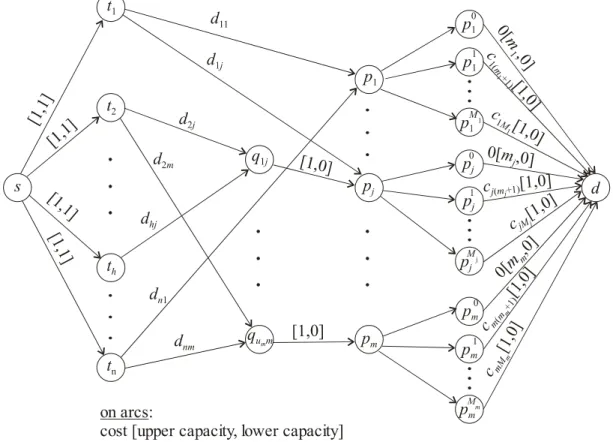
Provided there exists at least one feasible assignment for G1 ≤ G , the problem of finding the best 1

assignment with respect to G2 and G3, called problem (P), can be formulated as a bi-criteria

network flow problem in network N’ (see Fig. 5) obtained from N (shown in Fig. 1) by the following transformation:

the lower bounds on flows transmitted along all n entering arcs (s, th) are equal to one;

each vertex corresponding to processing unit pj (j=1,…,m) is followed by a new layer

composed of Mj–mj+1 vertices pvj (v=0,…,Mj–mj); each new vertex is connected by

an ingoing arc with p

v j p 0 j v j p

j and by an outgoing arc with d; the vertex corresponds to the

regular capacity m

p

j of the processing unit pj, while vertices (v=1,…,Mj–mj)

correspond to each unit capacity of pj, over mj and up to Mj; a unit capacity of pj is

considered as a copy of the processing unit pj; the capacities of new arcs are unlimited for

(pj,pvj) (j=1,…,m; v=0,…,Mj–mj) and κ(p0j,d)=mj, κ(pvj,d)=1 (j=1,…,m; v=1,…,Mj–mj);

the lower bound on all new arc flows is equal to zero;

two types of costs are associated with unit flows through arcs of network N’:

o costs of processing type, that is costs of unit flows through arcs ( ,d); they are equal

to 0 for ( ,d), and to marginal cost >0 for ( ,d), such that

≥ c (j=1,…,m; v=1,…,M v j p p 0 j p − +v mj ) (m v j j c ₊ v j ) (m v j j

c _{+ j( 1)} j–mj); these costs correspond to processing

costs of pj for its regular capacity (v=0) and for each additional unit capacity

(v=1,…,Mj–mj), respectively; the costs of the processing type on all other arcs are,

obviously, equal to zero;

o costs of dissatisfaction type, that is costs of unit flows through directly connecting arcs (th, pj) and indirectly connecting arcs (th, qij), equal to dhj (h=1,…,n, i=1,...,uj,

j=1,…,m); these costs correspond to dissatisfaction degrees of th for being assigned to

The two criteria associated with feasible flow Φ in network N’ are defined, respectively, as:

( ) ( )

w' c w' G₂ =

∑

_w'∈W'Φ

( ) ( )

w' d w' G₃ =

∑

_w'∈W'Φ

where W’ is the set of arcs w’ of N’, Φ (w’) is a flow through arc w’, c(w’) is a cost of the processing type for a unit flow through arc w’, and d(w’) is a cost of the dissatisfaction type for a unit flow through arc w’.

Fig. 5. The bi-criteria integer minimum cost flow problem in network N’

To verify that the bi-criteria network flow problem in network N’ corresponds to our problem (P), the following remarks may be useful:

1. The non-zero costs of the processing type and the non-zero costs of the dissatisfaction type concern different arcs in N’, that is, if c(w’)≠0 then d(w’)=0 and vice versa.

2. As the marginal cost of all additional copies of pj (j=1,…,m) is non-decreasing, it is

Φ(pj,pvj)=Φ( pvj,d)=1, while Φ( pj,pzj)=Φ (pzj,d)=0 for some z<v; this proves that G3

represents adequately the total cost of processing units.

Formally, a solution (flow) x* _{of problem (P) is non-dominated if there does not exist any other} feasible solution x such that Gl(x) ≤ Gl(x*), l=1,2, with at least one strict inequality. The set of all

non-dominated solutions of problem (P) will be denoted by ND(P). Each non-dominated solution

x* _{has its image in the criterion plane (G}

2×G3), denoted by G(∗). For the sake of simplicity, we will

use the notion of solution with respect to both x* _{and its image G}(∗)_{, unless a distinction will be}

necessary to avoid misunderstanding.

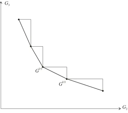
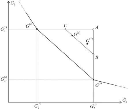
Fig. 6. Supported non-dominated solutions and potential regions ∆G(r)_G(s) _{of supported}

non-dominated solutions of problem (P)

It is well known that in multi-criteria discrete optimization problems, thus also in case of our problem (P), it is necessary to distinguish two kinds of non-dominated solutions (see, e.g. (Ulungu & Teghem, 1994)):

the set S(P) of supported non-dominated solutions which are optimal solutions of the parameterized single-objective problem (Pλ):

Minimize Gλ(x) = λ G2(x) + (1- λ) G3(x) (Pλ)

the set NS(P) = ND(P) \ S(P) of non-supported non-dominated solutions which cannot be found by solving problem (Pλ) for any λ∈(0, 1). These non-supported non-dominated

solutions are necessarily located in the triangles ∆G(r)_G(s) _{created in the criterion plane}

(G2×G3) by any two successive supported non-dominated points, as shown in Fig. 6.

In the following we show how to obtain the supported and the non-supported non-dominated solutions of problem (P) by exact methods. Specifically, in point 5.2, we use the bi-criteria network flow formulation of problem (P) in order to find all supported non-dominated solutions of (P), that is, optimal solutions of problem (Pλ). In order to find all non-supported non-dominated

solutions of (P) we propose in point 5.4 to use the well known exact method of Ulungu and Teghem (1995), for a bi-criteria basic assignment problem, within a branch and bound procedure. As the method of Ulungu and Teghem (1995) works on a matrix representation of the bi-criteria basic assignment problem, we represent our problem (P) in matrix terms in point 5.3.

Let us mention that, recently, Sodeno-Noda and Gonzalez-Martin (2001), and Figueira (2002) have proposed general algorithms for the bi-criteria integer minimum cost flow problem. While the first one involves a classic tool of network flow problems, such as the network simplex method, the second one proposes a branch and bound method for searching both supported and non-supported non-dominated solutions of a bi-criteria integer minimum cost flow problem. We decided to use, however, an intermediate, two-stage approach: a parametric network flow algorithm in order to find all supported non-dominated solutions, and then, a branch and bound method involving a simple procedure for bi-criteria basic assignment with a systematic check of incompatibility constraints in order to find all non-supported non-dominated solutions. In this way we are able to better exploit the specific structure of our problem including the constraints of a basic assignment problem and the specific incompatibility constraints.

5.2. Searching for supported non-dominated solutions of problem (P)

In order to find an optimal solution of the parameterized problem (Pλ), we will solve the

minimum cost network flow problem in network N’, where all the costs of the dissatisfaction type are multiplied by λ and all the costs of the processing type are multiplied by (1- λ). The obtained integer flow equal to n minimizes the objective function Gλ(x) = λ G2(x) + (1- λ) G3(x).

One can solve this network flow problem using a polynomial time algorithm, for example the simplex-based algorithm of Orlin (1997). It should be noticed, however, that if there exist alternative optimal solutions of problem (Pλ), they should all be discovered because they may

correspond to different supported non-dominated solutions of problem (P). Unfortunately, finding all alternative optima of problem (Pλ) may be time consuming.

Searching for supported non-dominated solutions of problem (P) proceeds as follows (see Ulungu and Teghem, 1995).

Let S denote a list of all supported non-dominated solutions already found. S is initialized by finding two non-dominated solutions of problem (Pλ), first for λ being very close to 1 (say 0.999)

and then for λ being very close to 0 (say 0.001).

In S, solutions are ordered according to increasing value of G2. Let {G(r), G(s)} denote two

consecutive solutions in S. Thus, G <G and > . In order to find new supported non-dominated solutions, one has to find all optimal solutions of problem (P

) r (

2 2(s) G3(r) G3(s)

λ) with the following

value of λ:

(

(s) (r)

) (

(r) (s)

)

) s ( ) r ( G G G G G G 3 3 2 2 3 3 − + − − = λ .

Let {G(t)_{, t=1,…,y} be a set of optimal solutions obtained in this way, ordered according to}

increasing value of G2. Two possible cases can arise:

{G(r)_,G(s)_}∩{G(t)_{, t=1,…,y} = ∅; then G}(t)_{, t=1,…,y, are new supported non-dominated}

solutions to be put in S; if y>2, then in further steps it will be necessary to consider the

pairs {G(r)_{, G}(1)_{} and {G}(y)_{, G}(s)_{}, while it will be possible to skip other pairs {G}(t)_{, G}(t+1)_}, t=2,…,y-1;

{G(r)_,G(s)_}⊂{G(t)_{, t=1,…,y}; if y>2, then G}(t)_{, t=2,…,y-1, are new supported}

non-dominated solutions to be put in S, however, they are not entering the pairs that should

be further checked for existence of new supported non-dominated solutions.

After solving (Pλ) for all consecutive pairs of solutions from S that may yield new supported

non-dominated solutions, the final list S = S(P), that is, it contains all supported non-dominated

solutions of problem (P).

5.3. Matrix representation of problem (P)

Problem (P) can also be represented as a generalized assignment problem, where assignments are done directly in a matrix whose rows correspond to tasks and columns to processing units. Each entry of the matrix is a cost of assignment of a task to a processing unit. The complete minimum

cost assignment corresponds to selection of n entries in the matrix that minimize the sum of the

entries while observing the imposed constraints.

As we are considering two criteria, each of them will be associated with a different cost matrix: criterion G2 with a matrix D of dissatisfaction type costs, and criterion G3 with a matrix C of

processing type costs. Both matrices are of the same dimension: n×π, where π = . In this representation, the first M

∑

=

m j 1Mj

1 columns of C and D correspond to copies of p1 , the following M2

columns to copies of p2, etc.

The entries of matrix D are defined as: Dhi = dh1 for i=1,…,M1, and Dhi = dh2 for

i=M1+1,…,M1+M2, and … Dhi = dhm for i=π −Mm+1,…,π; h=1,…,n. Remark that dissatisfaction

degrees of each particular task are identical for all copies of the same processing unit.

As the cost of each particular copy of a processing unit is the same for all tasks, the rows of matrix C are identical. Each row of matrix C is defined as: Ch = [0,…,0, ,…, ,0,…,0, ,…, ,…,0,…,0, ,…,c ], h=1,…,n,

where the number of zeroes is equal, respectively, to m 11 c c_1(M1−m1) c₂₁ c_2(M2−m2) c_{m1 ( )} m m m M m − 1, m2,…, mm.

Our bi-criteria assignment problem is clearly a generalization of the basic assignment problem, because in the former there are two, instead of one, objective functions and additional incompatibility constraints have to be considered. The constraints of the basic assignment problem impose that each task is assigned to exactly one processing unit and vice versa. This implies consideration of a square cost matrix. Therefore, if n<π, in order to represent our assignment problem as a generalization of the basic assignment problem, one has to augment the matrices D and C to the dimension π×π, by putting zeros in the empty rows. Of course, the assignments made in the rows n+1,…,π are dummy ones. As the costs of dummy tasks are all equal to zero, it is obvious that they do not affect the assignment of real tasks in the optimal solution.

We can use the matrix representation of problem (P) to give an equivalent formulation of (P) as a mathematical programming problem. We will give this equivalent formulation below in order to show the incompatibility constraints in terms of the matrix representation.

Let us define the decision variables as:

xhi =    ₊

_∑

− ₌ = otherwise. , 0 , where , processor of copy th to assigned been has task if , 1 t_h r p_j r _kj 1₁M_k i h=1,…, π, i=1,…, π,

Problem (P) can be expressed as follows: Minimize

( )

( )

_      = =

∑ ∑

∑ ∑

= = = = π π π π 1 1 3 1 1 2 h i hi hi h i hi hi x C G x D G x x subject to

_∑

π_i=1x_hi =1, h=1,…,π,

∑

π_h=1x_hi =1, i=1,…,π, xhi ∈{0, 1}, h=1,…,π, i=1,…, π,

and the incompatibility constraints 1 ≤

∑ ∑

∈Hlj ∈ j h i J hi x , =

{

∑

j−₌1₁ +1

∑

₌₁

}

k j k k k j M ,..., M J , H_lj =

{

h:t_h∈Q_lj

}

, j=1,…,m, l=1,...,uj,

where Qlj is the l-th incompatibility group of processing unit pj, , and x is the

vector of decision variables defining the assignment.

0

0

1 =

∑

k= Mk

Problem (P) is a bi-criteria 0-1 integer linear programming problem.

5.4. Searching for non-supported non-dominated solutions of problem (P)

After finding all supported non-dominated solutions contained in the list S = S(P), one can proceed to the search of non-supported non-dominated solutions of problem (P). These solutions are necessarily located in the triangles ∆G(r)_G(s) _{created in the criterion plane (G}

2×G3) by any two

supported non-dominated solutions being successive on the list S (see Fig. 6 and 7).

Ulungu and Teghem (1995) proposed an exact method of searching for supported non-dominated solutions of a bi-criteria basic assignment problem. It examines systematically the interior of all triangles ∆G(r)_G(s) _{using the well-known Hungarian method for optimization of}

some reduced assignment problems in the π×πmatrix:

DCλ = λD + (1-λ)C,

where, for the triangle ∆G(r)_G(s)_,

(

(s) (r)

) (

(r) (s)

)

) s ( ) r ( G G G G G G 3 3 2 2 3 3 − + − − = λ . To set up a reduced assignment problem, Ulungu and Teghem use properties of dual variables of the linear relaxation of problem (Pλ) considered without the incompatibility constraints. Each time the Hungarian

method is applied, it is necessary to obtain all alternative optimal solutions because they may correspond to different values of G2, G3. An enumeration procedure is thus needed to examine all

such costs is greater than π. If the number of zero reduced costs is much greater than π, this enumeration procedure is time consuming.

Fig. 7. Searching for non-supported non-dominated solutions of problem (P)

Each non-supported non-dominated solution resulting from the above procedure, say G(q), included in a triangle ∆G(r)_G(s)_{, has to be checked if it satisfies the incompatibility constraints. If it}

is the case, G(q) _{is included in set NS(P) of non-supported non-dominated solutions of problem}

(P). Otherwise, G(q) _{becomes a starting solution for a branch and bound procedure that tries to}

find a feasible solution of problem (P) located in the corresponding triangle ∆G(r)_G(s)_{. This}

procedure, called ‘Explore NS’, is described below. Procedure ‘Explore NS’

Step 1. Take a non-supported non-dominated solution obtained by the method of Ulungu and Teghem, say G(q)_{, included in the triangle ∆G}(r)_G(s) _{and such that G}(q) _{defines in the}

corresponding matrix DCλ an assignment x(q) which does not satisfy the incompatibility

constraints.

Step 2. Let CLUB represent the current least upper bound on the optimal assignment in matrix

DCλ which satisfies the incompatibility constraints and belongs to the triangle ∆G(r)G(s).

Set CLUB= ( ), that is to the value of the worst point in the triangle

3 ) ( 2s (1 )G r G λ λ + −

∆G(r)_G(s) _{(point A in Fig. 7). Make solution G}(q) _{and the corresponding assignment in}

matrix DCλ the root of the branching tree. Let also L(DCλ) represent a lower bound on the

optimal assignment in matrix DCλ which satisfies the incompatibility constraints and

belongs to the triangle ∆G(r)_G(s)_{. Set L(DC}

λ)=Gλ(x(q)).

Step 3. Identify the incompatibility constraints that are not satisfied by solution G(q)_{, that is such} j∗∈{1,…,m} and l∗_∈{1,...,u

j} that . Let min >1 and

denote the corresponding j

1 ) ( _>

∑ ∑

∗ ∗ ∗ ∈H_{l j} ∈ _j h i J q hi x x k j l j H h i J q hi l, j _=       

∑ ∑

∗ ∗ ∗ ∗ ∗ ∈ ∈ ) ( ∗ _{by φ, and l}∗ _{by ψ.}

Step 4. Branch into k assignment subproblems and set for subproblem 1, matrix element

( )

1 1 =∞

1 _{h ,i}

DC_λ , for subproblem 2, _DC2

(

_h2_,i2

)

=∞

λ , and so on, until subproblem k,

(

k k

)

=∞ k _{h ,i} DC_λ h , x q hi) = 1 (

. Setting a matrix element on infinity means that the corresponding assignment is forbidden. The co-ordinates of the assignments forbidden in particular subproblems are different and numbered pairs of indices (h1,i1), (h2,i2), …, (hk,ik) for which ∈H_ψφ, i∈J_φ.

Step 5. Solve the k new assignment problems without the incompatibility constraints by the Hungarian method. Each optimal solution is a lower bound _L

( )

_DCf

λ , f=1,…,k, for the

corresponding subproblem. If for a subproblem there are alternative optima, they should all be identified.

Step 6. If there are one or more solutions from step 5 that satisfy the incompatibility constraints and are located in the triangle ∆G(r)_G(s)_{, and if the smallest L}

( )

_DCf

λ for these solutions,

say L

( )

DC_λ∗ , is smaller than CLUB, set CLUB=L

( )

DC_λ∗ and save the corresponding solution G . Otherwise, CLUB remains unchanged. (∗)

Step 7. If CLUB is less than the lower bounds on all unexplored subproblems, then solution corresponding to CLUB is a candidate to be included in set NS(P), so stop; otherwise, go to step 8. By unexplored subproblems, we mean subproblems, corresponding to solutions with non-satisfied incompatibility constraints, that have not been branched into further subproblems.

) (∗

G

Step 8. From the set of all unexplored subproblems with lower bounds less than CLUB, select subproblem G(#) _{with the smallest lower bound for further branching. Substitute G}(q) _and

The above branch and bound procedure needs some comments:

1. ‘Explore NS’ solves the easier assignment problem that does not respect the incompatibility constraints and then systematically forbids assignments violating the incompatibility constraints until finally an optimal assignment satisfying the incompatibility constraints is obtained (if one exists in the triangle).

2. The branching into subproblems in Step 3 is organized such that each subproblem gets one forbidden assignment, from among assignments of one incompatibility constraint that was violated to a minimum extent in solution G(q)_{, that is a incompatibility constraint having the}

minimum number k>1 of tasks assigned to processing units. Note that there is no need to check out the subproblems arising from other incompatibility constraints violated in solution

G(q) _{(if there are any). It would also lead to the optimal solution, however, the search strategy}

of the solution space would be of the “breadth-first-search” type. Our strategy of branching for only one violated incompatibility constraint is of the “depth-first-search” type – it has been acknowledged to be more efficient and less memory-demanding.

3. If subproblems in Step 4 have many alternative optima then this step can be time-consuming. In practice, however, the initial interval between the current least upper bound CLUB and the lower bound on the optimal assignment provided by the Hungarian method is rather narrow which permits to eliminate many subproblems from further exploration.

4. The systematic search of the solution space by ‘Explore NS’ guarantees that if for a given G(q)

there exists a non-supported non-dominated solution of problem (P) in the triangle ABC (see Fig. 6), then it will be found.

5. If CLUB has not been changed during the branch and bound procedure, this means that no non-supported non-dominated solution of problem (P) can be found starting from G(q)_.

Otherwise, solution G corresponding to a final value of CLUB is included in NS(P) if it is not dominated by any other solution from this set; at the same time, the solutions from NS(P) dominated by are eliminated.

) (∗ ) (∗ G 6. Numerical examples

6.1. Example with a blocking configuration

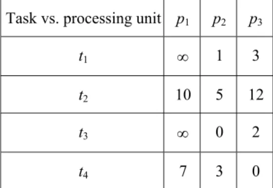
Let us consider the assignment of 5 tasks to 3 processing units with regular capacity equal to 1. The capacity of processing unit p1 cannot be increased, while the capacity of p2 and p3 can be

Table 1. The processing costs of tasks by the processing units

p1 p2 p3

Until the regular capacity: 0 0 0 The first additional task: ∞ 10 25

The dissatisfaction degrees of particular tasks for being assigned to particular processing units are given in Table 2.

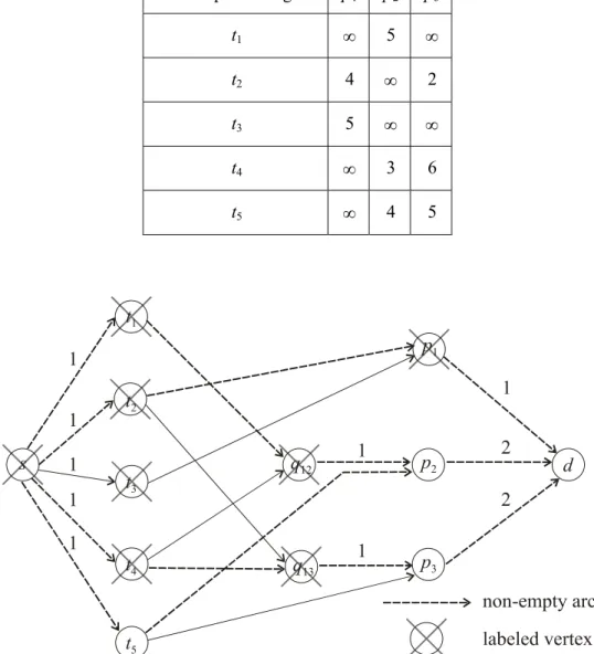
Table 2. The dissatisfaction degrees of tasks for being assigned to processing units Task vs. processing unit p1 p2 p3

t1 ∞ 5 ∞

t2 4 ∞ 2

t3 5 ∞ ∞

t4 ∞ 3 6

t5 ∞ 4 5

The assignment of tasks to processing units has to respect some incompatibility constraints. One incompatibility group is defined for processing unit p2 and another for p3; they are as follows:

Q12 = {t1, t4}, Q13 = {t2, t4}.

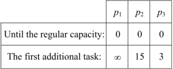
The problem of finding a feasible assignment of tasks to processing units, defined above, can be formulated as a problem of finding a maximum integer flow in network N•shown in Fig. 8. The maximum integer flow in network N• has value 4, which is less than the number of all tasks. Thus, the assignment problem has no feasible solution for the above constraints. There are 8 alternative flows of value 4, corresponding to one non-assigned task t1, t2, t3 or t4, combined with

a possibility of assigning task t5 either to p2 or p3; let us denote them by t1-t5/p2, t1-t5/p3, t2-t5/p2, t2 -t5/p3, t3-t5/p2, t3-t5/p3, t4-t5/p2, t4-t5/p3, respectively; the flow t3-t5/p2 is shown in Fig. 8.

We will show the blocking configuration for the maximum flow presented in Fig. 8. The characteristic sets introduced in point 3.2 are as follows:

Tx={t5}, Bµ={t2}, Bz={t1, t4}, Bρ={t3},

C=∅, C’={q12, q13}, C’’=∅, D={p1}, D’={p2, p3}, D’’=∅.

The blocking configuration <B, C’, D> for any maximum flow in N• is equal to: <{t1, t2, t3, t4}, {q12, q13}, {p1}>

According to point 3.4, the following actions of unblocking are possible (the initial flow is t3-t5/p2): (a) action of type 1: augment by one the capacity of p1,

(b) action of type 2: allow p3 to process t1 directly, (c) action of type 2: allow p3 to process t3 directly,

(d) action of type 3: allow p3 to process directly t2 that it was able to process indirectly only, (e) action of type 3: allow p3 to process directly t4 that it was able to process indirectly only, (f) action of type 4: augment by one the capacity of p2 and allow it to process t2 directly, (g) action of type 4: augment by one the capacity of p2 and allow it to process t3 directly, (h) action of type 4: augment by one the capacity of p2 and allow it to process directly t1 that

it was able to process indirectly only,

(i) action of type 4: augment by one the capacity of p2 and allow it to process directly t4 that

it was able to process indirectly only,

(j) action of type 6 (action 2 for alternative flow t2-t5/p3): allow p2 to process t2 directly, (k) action of type 6 (action 2 for alternative flow t3-t5/p3): allow p2 to process t3 directly,