Poverty Dynamics in Peru, 1997-1999

D

OCUMENT DE

T

RAVAIL

DT/2001/09

Poverty Dynamics in Peru, 1997-1999

RESUME

Comment la pauvreté a-t-elle évolué pendant les années 1997-1999, période durant laquelle les performances de l’économie péruvienne se sont sérieusement détériorées sous l’effet négatif de la crise financière internationale ? La réponse à cette question se base traditionnellement sur des comparaisons en coupe instantanée des indicateurs de pauvreté. Dans ce rapport, nous élargissons l’analyse en examinant tout d’abord la fiabilité de ce type de comparaisons à travers la prise en compte des erreurs d’échantillonnage, et ensuite en analysant les transitions de pauvreté des ménages présents durant les trois années de notre panel. En plus des matrices de mobilité de transitions, nous avons calculé un indice de mobilité plus récent proposé par Fields et Ok et estimé un modèle logit multinomial de transition de pauvreté, comprenant non seulement les caractéristiques des individus et des ménages, mais aussi les variables géographiques locales concernant principalement la fourniture des biens publics. Enfin, les programmes de lutte contre la pauvreté ont été évalués sur la base d’approches statiques et dynamiques de la pauvreté.

ABSTRACT

How has poverty changed during the 1997-99 period, when the Peruvian economic performance deteriorated seriously under the negative impact of the international financial crisis? The answer to this question has traditionally relied on cross-section comparisons of poverty indicators. In this paper we extend the analysis first by examining the robustness of these kind of comparisons by considering sampling errors and stochastic dominance and second, by analyzing poverty transitions for households present in the three years of our panel data. Besides transition mobility matrices, we calculated the newer economic mobility index proposed by Fields and Ok and estimated a multinomial logit model of poverty transitions including not only individual and household characteristics but also local geographical variables concerning mainly the provision of public goods. Finally, anti-poverty programs were then evaluated on the basis of static and dynamic poverty approaches.

Theme: Welfare, income distribution and poverty

Keywords: poverty dynamics, inequality, Peru, multinomial logit JEL-Code: I32, D63, D31

This paper was presented at the LACEA / IDB / World Bank on inequality and Poverty held in October 11, 2000 at Rio de Janeiro, Brazil.

Index

INTRODUCTION ... 6

1. CROSS-SECTION EVOLUTION OF POVERTY AND INEQUALITY ... 7

2. CROSS-SECTION INEQUALITY COMPARISONS ... 9

3. STOCHASTIC POVERTY DOMINANCE... 9

4. STOCHASTIC INEQUALITY DOMINANCE ... 11

5. KERNEL EXPENDITURES DISTRIBUTION IN PERU 1997, 1999... 11

6. ANOTHER LOOK TO THE SHRINKING MIDDLE CLASS: POLARIZATION OF THE INCOME DISTRIBUTION ... 13

7. POVERTY AND INCOME TRANSITIONS ... 14

8. THE STEADY STATE POVERTY RATE ... 16

9. PERMANENT AND TRANSIENT POVERTY IN PERU... 17

10. SENSIBILITY TO POVERTY LINE AND MEASUREMENT ERRORS... 19

11. PROFILE OF POVERTY TRANSITIONS... 20

12. POVERTY AND INEQUALITY DECOMPOSITIONS... 21

13. INEQUALITY DECOMPOSITION BETWEEN AND WITHIN GROUPS... 24

14. DECOMPOSING INCOME MOBILITY IN PANEL DATA: FIELDS/OK’S GROWTH AND “EXCHANGE” MOBILITY... 25

15. DIRECTIONAL MOBILITY INDEX... 26

16. MODELLING POVERTY TRANSITIONS... 27

17. THE EXPLANATORY VARIABLES ... 29

18. THE MULTINOMIAL UNORDERED REGRESSION MODEL ... 30

19. REGRESSION RESULTS ... 30

20. POVERTY TRANSITIONS AND POVERTY REDUCTION POLICIES ... 32

CONCLUSION... 35

BIBLIOGRAPHY ... 36

Tables Index

Table n° 1-1: Foster-Greer-Thorbecke poverty measures, Peru 1997-1999...6

Table n° 2-1: Gini coefficients ...8

Table n° 7-1: Poverty transitions 1997-1999 ... 14

Table n° 7-2: Poverty transitions 1997/1999 ... 14

Table n° 9-1: Permanent and transient poverty ... 16

Table n° 10-1: Sensibility of poverty transitions to poverty line and measurement errors ... 18

Table n° 10-2 / Table n° 10-3: Quintile transition matrix... 19

Table n° 10-4: Transition matrix mobility indicators ... 19

Table n° 12-1: Decomposition of poverty changes into growth and inequality effects ... 22

Table n° 13-1: Theil inequality between groups, level and % of total inequality... 24

Table n° 15-1: Fields/Ok income mobility index ... 26

Table n° 17-1: Poverty transitions 98-99 (weighted) ... 28

Table n° 20-1: Targeting indicators for policies to fight poverty... 32

Table n° 20-2: Targeting indicators and poverty transitions ... 32

Figures Index

Figure n° 3-2: Cumulative distributions of rural and urban household per capita expenditure 1997, 1998 and 1999 10 Figure n° 4-1: Vertical distance of the Lorenz curves from diagonal ... 11

Figure n° 5-1: National Kernel densities for household per capita real expenditures... 12

Figure n° 5-2: Urban and rural Kernel densities for household per capita real expenditures ... 12

Figure n° 6-1: Inequality and polarization: a graphical representation ... 13

Figure n° 8-1: Flows into and out of poverty, 1997-1999 ... 16

Figure n° 15-1: Directional and absolute mobility... 27

Appendices

Appendix n° 2 : Testing significance of poverty rates changes ... 37

Appendix n° 3 : Poverty transitions 1997-1998... 37

Appendix n° 4: Exits from poverty according to the distance respect the poverty line ... 39

Appendix n° 5: Entries to poverty according to the distance respect the poverty line ... 39

Appendix n° 6: Gini coefficients with it confidence intervals... 40

Appendix n° 7: Poverty Transitions 1997-1998 & Characteristic in 1997 (%) ... 41

Appendix n° 8: Variables in the regression ... 45

Appendix n° 9: Poverty transitions 98-99 (weighted) ... 47

Appendix n° 10: Multinomial regression ... 48

Appendix n° 11: Hausman tests of IIA assumption... 49

Appendix n° 12: Small-Hsiao tests of IIA assumption ... 49

INTRODUCTION

The Peruvian economy experienced a period of rapid expansion from 1993-1997 (exceeding 6% per year on average) but growth then slowed down significantly, similarly to the other countries in the sub-region hit by the Asian crisis. It is stagnating at 0.5% and per capita household spending fell by 8% from 1997 to 1999. There have been far-reaching macroeconomic disruptions in Peru since 1991, marking radical changes in its economic policy: most State enterprises were privatized; subsidies and price control were abolished; the labor market was liberalized whilst social spending was multiplied by three from 1993 to 1998 (from $63 to $174 per capita). In this new unfavorable macroeconomic environment, the insistent problems of poverty that concern nearly four out of ten Peruvians (six out of ten in rural areas) and the continuing extremely high levels of inequality (Gini coefficient: 0.48) have come back onto the agenda in academic and political circles. In Peru, certain people maintain that the fact that the indicators have not improved challenges the effectiveness of policies aimed at fighting poverty and the capacity of economic growth to reduce inequality and poverty.

However, the disappointing results obtained in terms of living standards and inequalities are judged from a static standpoint, by comparing indicators in a given year with those of previous years. Net balances of poverty are taken into consideration and not the households’ trajectories over a period of time. Thus, important questions remain unanswered. What share of the population is in a state of permanent poverty and what percentage of the poor in a given year are « transient poor »? Do the permanently poor have any particular characteristics that differ from those of the transient poor? In what way does this dynamic approach to poverty lead to rethinking on policies to combat poverty? Few developing countries are equipped to answer these questions as this implies being able to monitor the same households on a large scale over a period of time, and the necessary surveys are quite rare in these countries.

However, Peru has recently set up a panel of households with national coverage (see box). Taking advantage of this new database, a joint study covering all the above questions was carried out by the Peruvian National Institute of Statistics and Information Technology (INEI) and DIAL, on poverty dynamics for the period 1997-1999. The main results are presented in the following pages.

Data from ENAHO panel

As of 1996 INEI, with support from the IDB in the framework of the MECOVI program for the improvement of household surveys on living standards, has a new database at its disposal on recent trends in poverty in Peru. The national household surveys (ENAHO) that we use were designed from the outset to include a significant panel base, with national coverage. Conclusions can be drawn with respect to seven geographical zones, and to urban and rural areas. The survey concerned 3,100 households and nearly 15,000 individuals over the complete period 1997-1999. The panel base represents a little over 50% of the total sample. Apart from information on housing and demographical data concerning the individuals, the surveys included a section on education, health, expenditure, income, employment, etc. The surveys analyzed were carried out in the last quarter of 1997, 1998 and 1999.

Data from these surveys was completed with data from local administration censuses (“municipalidades”) carried out in 1994 and 1997. It was thus possible to include not only the characteristics of the households and the individuals but also local variables, such as provision of public services (health and education), distance, quantity and quality of roads and economic density.

1. CROSS-SECTION EVOLUTION OF POVERTY AND INEQUALITY

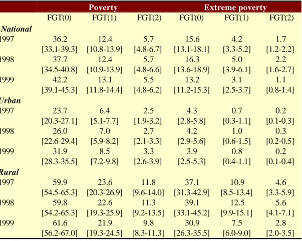
The question whether poverty has increased or diminished over the last years has raised great concern among Peruvian politicians and researchers. We will first examine this issue in the usual way, which is to say by comparing poverty incidence using a cross-section approach. According to this approach, poverty headcount increased slightly between 1997 and 1998 (from 36.2% to 37.7%). In spite of a 6% decline in average household per capita real expenditure, neither the depth of poverty (average distance from the poverty line) nor poverty severity changed during these years (see table below). A major upsurge in national poverty rates occurred in 1999 when the incidence of poverty jumped to 42.2% without, once again, implying significant changes in poverty severity or inequality among the poor. This may suggest that there were important redistributive effects.

Table n° 1-1: Foster-Greer-Thorbecke poverty measures, Peru 1997-1999

Poverty Extreme poverty

FGT(0) FGT(1) FGT(2) FGT(0) FGT(1) FGT(2) National 1997 36.2 [33.1-39.3] 12.4 [10.8-13.9] 5.7 [4.8-6.7] 15.6 [13.1-18.1] 4.2 [3.3-5.2] 1.7 [1.2-2.2] 1998 37.7 [34.5-40.8] 12.4 [10.9-13.9] 5.7 [4.8-6.6] 16.3 [13.6-18.9] 5.0 [3.9-6.1] 2.2 [1.6-2.7] 1999 42.2 [39.1-45.3] 13.1 [11.8-14.4] 5.5 [4.8-6.2] 13.2 [11.2-15.3] 3.1 [2.5-3.7] 1.1 [0.8-1.4] Urban 1997 23.7 [20.3-27.1] 6.4 [5.1-7.7] 2.5 [1.9-3.2] 4.3 [2.8-5.8] 0.7 [0.3-1.1] 0.2 [0.1-0.3] 1998 26.0 [22.6-29.4] 7.0 [5.9-8.2] 2.7 [2.1-3.3] 4.2 [2.9-5.6] 1.0 [0.6-1.5] 0.3 [0.2-0.5] 1999 31.9 [28.3-35.5] 8.5 [7.2-9.8] 3.3 [2.6-3.9] 3.9 [2.5-5.3] 0.8 [0.4-1.1] 0.2 [0.1-0.4] Rural 1997 59.9 [54.5-65.3] 23.6 [20.3-26.9] 11.8 [9.6-14.0] 37.1 [31.3-42.9] 10.9 [8.5-13.4] 4.6 [3.3-5.9] 1998 59.8 [54.2-65.3] 22.6 [19.3-25.9] 11.3 [9.2-13.5] 39.1 [33.1-45.2] 12.5 [9.9-15.1] 5.6 [4.1-7.1] 1999 61.6 [56.2-67.0] 21.9 [19.3-24.5] 9.8 [8.3-11.3] 30.9 [26.3-35.5] 7.5 [6.0-9.0] 2.8 [2.0-3.5]

Source: Our estimation from ENAHO 1997-IV, 1998-IV and 1999-IV.

FGT(0): headcount ratio

FGT(1): average normalized poverty gap

FGT(2): average squared normalized poverty gap 95% confidence intervals in parentheses

A more contrasted picture appears when poverty rates are broken down by rural/urban areas and by regions. First we find that there are very significant differences in poverty levels between rural and urban areas. Six out of ten Peruvians living in rural areas are poor, while this situation concerns “only” around three in ten urban individuals. However, it appears that poverty increase over the 1997-1999 period was an almost exclusively urban phenomena, somewhat concentrated in the Costa regions. Poverty incidence increased by around 7 percentage points in the capital Lima and in the urban coast (representing 52% and 39% change, respectively). Rural areas and Sierra and Selva regions recorded relatively small poverty changes during the examined period. Of the approximately one and half million increase in the number of poor between 1997 and 1999, 43% came from Lima and 30% from the urban coast. Thus, increase in poverty was essentially an urban phenomenon affecting the population living in large cities. This has led to a moderate deconcentration of poverty in rural compared to urban areas. The share of rural poor fell from 57% to 50% so that poverty is no longer “a rural problem” as it was in the past. Gaps remained at the same levels in terms of severity or intensity of poverty (FGT1 and FGT2 poverty measures) (see graph and table below). Urban poverty appears to be highly cyclical (a World Bank study showed that during the 1994-1997 high growth period urban poverty declined by 13% while rural poverty diminished by only 4% (World Bank, 1999:12).

Contrasting with the rise in overall poverty, the extreme poverty rate (household expenditure below basic food consumption equivalent to the 3,318 kcal. requirement), after rising slightly in 1998 declined by almost 3 percentage points in 1999 (from 16.3% to 13.2%). Extreme poverty in Peru is very much a rural phenomenon: eight out of 10 extreme poor are in households living in rural areas (which only account for 35% of total population); the remaining 20% are in urban dwellings, mostly outside the capital. The rural Sierra alone accounts for around 60% of the extreme poor in Peru (its population share is 22%). It was also the rural Sierra, by far the poorest region in Peru, that most benefited from the reduction in extreme poverty: around 80% of the decline concerned this region where the share of extreme poor diminished from 64% to 59% between 1998 and 1999, and the poverty incidence plumbed from 43.4% to 35.3%.

However, since household expenditures come from statistical surveys, differences in poverty rates must be evaluated taking into account sampling design. First, we estimated confidence intervals for each of the FGT poverty measures, then we performed t-tests for the null hypothesis that poverty incidence had not changed. Our results show (see appendix) that poverty headcount in 1999 was significantly higher than in 1997 and 1998 (t-test for difference in poverty headcount between 1997 and 1998 was statistically different from zero only at a 24% level of confidence). These results apply at national and urban levels. No significant changes in poverty rates in the 1997-99 period were found in rural areas (poverty rate was 1.7 percentage points higher in 1999 than in 1998 but, because of sampling size and design, standard errors are also important, almost twice those prevalent for urban areas (see table in the appendix). This means that poverty increases need to be greater than 2.4, 3.2 or 4.3 percentage points at the national, urban and rural levels respectively, in order to be considered as statistically significant. It should be noted that the range of confidence intervals is not necessarily the same for all regions. Such sampling errors are very often ignored in cross section poverty comparisons and in this sense their conclusions are not necessarily firmly established on statistical grounds.

2. CROSS-SECTION INEQUALITY COMPARISONS

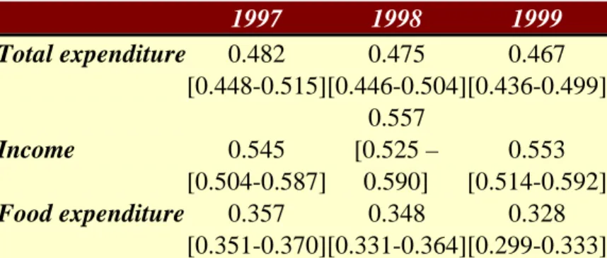
How did inequality fare during this period, particularly in 1999 when poverty increased significantly? Table 2-1 below and other regional disaggregated figures shown in the appendix suggest a reduction in inequality for household expenditure both in 1998 and 1999 but an increase in income inequality. Nonetheless, changes in Gini coefficients are relatively small, making it difficult to establish a general downward tendency; it can be observed that 95% confidence intervals for Gini coefficients overlap in all cases. Similarly, no clear-cut tendency can be discerned in any of the regional breakdowns reported in the appendix (Sierra and rural Gini coefficients were reduced by 10% and 6% but, again, confidence intervals overlap). A more robust cross section inequality analysis is carried out in the next section.

Table n° 2-1: Gini coefficients

1997 1998 1999 Total expenditure 0.482 [0.448-0.515] 0.475 [0.446-0.504] 0.467 [0.436-0.499] Income 0.545 [0.504-0.587] 0.557 [0.525 – 0.590] 0.553 [0.514-0.592] Food expenditure 0.357 [0.351-0.370] 0.348 [0.331-0.364] 0.328 [0.299-0.333]

Source: Our estimation from ENAHO 1997-IV, 1998-IV and 1999-IV. Weighted estimates for panel households at the individual level. 95% confidence intervals are bootstrap estimates.

3. STOCHASTIC POVERTY DOMINANCE

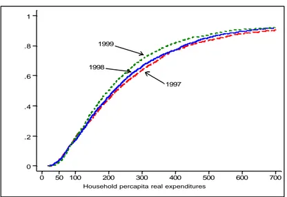
Since there is no single way to determine poverty lines and, more fundamentally considering that poverty is not a discrete phenomenon, cross-section comparisons of poverty rates must be completed by an examination of the whole distribution using the theory of stochastic dominance. This serves to evaluate the robustness of the conclusions made in the preceding analysis. In the graphics below, we show the cumulative density functions of real household per capita expenditure (at 1999 prices) for the overall population and separately for urban and rural populations. As before, only panel households are considered.

Figure n° 3-1: Cumulative distributions of household per capita expenditure 1997, 1998and 1999

At first sight, it seemed that the 1997 distribution dominated slightly the 1998 distribution and very clearly the 1999 distribution. The crossings of the cdf occurs either at the lower or at the upper segments of the distribution, outside the interval containing all range of plausible poverty lines. However, a Kolmogorov test for the similarity between each couple of distributions do not allow for the rejection of the null hypothesis in any of each comparison (1997/1998, 1998/1999, and 1997/1999) at the 1% or at the 5% confidence level1_{. However, things were not so} clear-cut for extreme poverty. Up to a real per capita household expenditure of around S/90 the 1999 distribution dominated the preceding years distributions2_{. This was reflected in the reduction of extreme} poverty rates in 1999 compared with the other two year in our period. In other words, this result is robust regardless of the way in which this extreme poverty line is determined.

With respect to urban households, the three cumulative distributions were almost the same up to S/100 soles. Over this amount the 1999 distribution was dominated by the 1997 and 1998 distributions. Poverty in urban areas undoubtedly increased steadily in 1998 and especially in 1999. The very significant decline in real expenditure for the segments near half of the distribution should also be noted. Concerning rural areas, the figure below shows that no robust conclusions can be put forward since all three distributions were extremely close to each other.

Figure n° 3-2: Cumulative distributions of rural and urban household per capita expenditure 1997, 1998 and 1999

1. Maximum absolute distances between distributions were 0.0332, 0.0247 and 0.162 for the 99/97, 99/98 and 97/98 cdf respectively. Critical values for Kolmogorov distribution (defined by c√ (n1+n2)/(n1*n2), where c is 1.36 or 1.63 according to 5% or 1% confidence level) at 1% confidence level is 0.04142 and 0.03456 for the 5% level.

2. In determining the critical poverty lines (crossing points in the cdf distributions) we use the DAD software, developed by CREFA.

1997

Household percapita real expenditures

0 50 100 200 300 400 500 600 700 0 .2 .4 .6 .8 1 1998 1999 1998 1999 1997

Urban households real expenditures

50 100 200 300 400 500 600 700 0 .1 .2 .3 .4 .5 .6 .7 .8 .9 1998 1997 1999

Rural households real expenditures

50 100 150 200 250 300 350 400 450 500 0 .1 .2 .3 .4 .5 .6 .7 .8 .9 1

4. STOCHASTIC INEQUALITY DOMINANCE

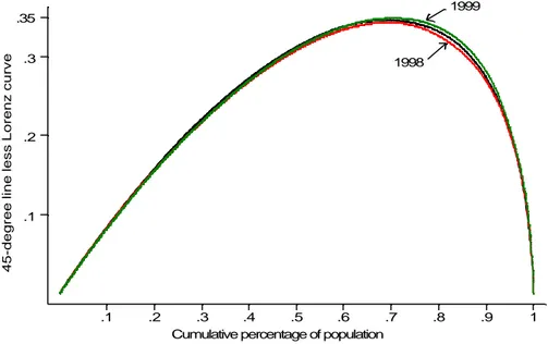
As can be appreciated in the graphic below, Lorenz curves for household expenditures for each year over the 1997-99 period are not only very near each other but they cross in several points. We cannot therefore conclude that there was an increase in inequality in Peru during the 1997-1999 period.

Figure n° 4-1: Vertical distance of the Lorenz curves from diagonal

1999

1998

45-degree line less Lorenz curve

Cumulative percentage of population

.1 .2 .3 .4 .5 .6 .7 .8 .9 1

.1 .2 .3 .35

5. KERNEL EXPENDITURES DISTRIBUTION IN PERU 1997, 1999

So far we have seen that inequality at the national level, as measured by the Gini coefficient, slightly diminished between 1997 and 1999 whilst poverty incidence significantly increased. Contrasted pictures appeared when we distinguished urban from rural areas. Inequality was constant in urban areas whereas it diminished in rural areas. Inversely, poverty increases revealed to be an almost entirely urban phenomenon while it remained fairly unchanged in rural areas.

However, one single parameter (i.e. Gini, Po) can hardly describe the whole distribution of households’ expenditures. More comprehensive indicators or devices are needed if we want to know which segment of the distribution experienced greatest changes and in what direction they moved. This may enable to answer relevant questions like whether or not the middle class is vanishing, making the 1999 distribution more polarized. Lorenz curves and household expenditure cumulative density functions were used as a first approach in examining stochastic dominance. Though (separately) more informative (spread and level), they give no clue at once about the tendency towards bimodality, nor they reveal changes in levels and the direction of shifts. Using kernel density estimation that provides a picture of the whole distribution can do this3_{. For each expenditure level, its associated frequency is shown graphically so we can simultaneously} examine changes in the level, tendency towards modality and spread of the expenditure distribution.

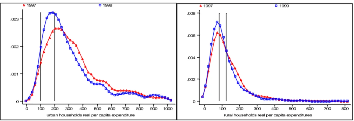
In figure bellow we have drawn kernel densities for 1997, 1998 and 1999 household expenditures with vertical lines representing grossly poverty lines (the lower one is extreme poverty). We can clearly see that the distribution has flattened over the 300-500 soles range, which corresponds approximatively to the richest 6th to 9th deciles. The increase in the density below the poverty lines that we observe particularly between 1998 and 1999 comes essentially from this segment of the distribution. Of course, since we are dealing with cross section data, this deformation of the distribution does not implies that there was income mobility of households from this deciles to the poorest ones. Does this pattern hold also for both rural and urban areas? The answer is no as is shown below.

Figure n° 5-1: National Kernel densities for household per capita real expenditures

household real per capita expenditure

1997 1999 1998 0 100 200 300 400 500 600 700 800 900 1000 0 .002 .004

In urban areas there is a leftward shift of most segments of the distribution, with the exception of the poorest households. The proportion of households around the poverty line increased significantly, particularly that of already poor households whereas it diminished for higher income households. In rural areas there was an increase in the extreme poor category coming both from poor and non-poor households. Note that the rural distribution seems far more unequal than the urban distribution of household's consumption expenditures4_.

Figure n° 5-2: Urban and rural Kernel densities for household per capita real expenditures

1997 1999 0 100 200 300 400 500 600 700 800 900 1000 0 .001 .002 .003

urban households real per capita expenditure rural households real per capita expenditures

1997 1999 0 100 200 300 400 500 600 700 800 0 .002 .004 .006 .008

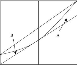
6. ANOTHER LOOK TO THE SHRINKING MIDDLE CLASS: POLARIZATION OF THE INCOME DISTRIBUTION

Does the decline in mean household incomes and expenditures had implied a tendency towards polarization putting the middle class under stress? One can wonder if the evolution of inequality in Peru was concomitant with a reduction of the degree of polarization of the distribution. An additional, though different question is whether there is a tendency towards bipolarization of the distribution, which is what is expected if the middle class is disappearing5

. Wolfson showed that the standard inequality indicator (the Gini coefficient) is not able to account for the polarization phenomenon, which implies a tendency toward the bi-modality of the distribution (Wolfson, 1997). One can have a curve of Lorenz more close to the diagonal in a bi-modal distribution than in the case of a Lorenz curve characterized by a more uniform distribution. The concepts of inequality and polarization are therefore two different concepts6

. The quoted author proposes an indicator of polarization that relies on a transformation of the Gini coefficient. He adds a tangent curve to the curve of Lorenz to the median while prolonging coordinates downwards. The surface given by A+B indicates the degree of polarization.

Figure n° 6-1: Inequality and polarization: a graphical representation

A B

The formula for the evaluation of this surface is:

P= 2(2T-Gini)/mtan Mtan = median tangent = median/mean

T= "the area of the trapezoid defined by the 45 degree line and the median tangent = the vertical distance between the Lorenz curve and the 45 degree line at the 50th percentile = 0.5 - L(5) = the difference between 50% and the income share of the bottom half of the population ". (Wolfson 1997: 15).

5. Birdsall, Graham, and Pettinato (2000) has proposed to compare the median income of the population that generates the top 50 percent of total income to the median income for the total population as an indicator of stress in the middle strata.

6. Esteban, J., C. Gradin, D. Ray (1999): « Extensions of a measure of polarization with an application to the income distribution of five OECD countries », Syracuse University, WP n°218.

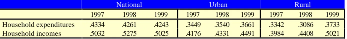
Tableau n° 6-1 : Polarisation coefficients

National Urban Rural

1997 1998 1999 1997 1998 1999 1997 1998 1999

Household expenditures .4334 .4261 .4243 .3449 .3540 .3661 .3342 .3086 .3733

Household incomes .5032 .5275 .5025 .4176 .4331 .4491 .3984 .4408 .5021

Source: Our estimation from ENAHO 1997-IV, 1998-IV and 1999-IV. Weighted estimates for panel households at the

individual level.

At the national level there is no tendency in the polarization index but there was a 12% increase in rural areas and 6% in urban areas. Notice that the degree of polarization is very similar in both areas. The increase in polarization was more pronounced in rural areas when considering household income instead of expenditures.

7. POVERTY AND INCOME TRANSITIONS

The incidence of poverty rose from 37.3% in 1997 to 39.2% in 1998 for the households in the panel and again to 42.7% in 1999. These increases may seem very moderate considering that per capita spending fell by about 6% in the panel for two consecutive years. Monitoring the trajectories of the same households over a period of time, hence distinguishing between people going into and out of poverty, revealed a more complex picture and qualifies the relative immobility of the static indicators of the net balance of poverty.

Panel surveys allow us to follow the same household across different time periods. A synthetic means of assessing flows between poverty and non-poverty is to build transition matrices in which the lines refer to the situation of the individuals in the first year, whereas the columns refer to the situation of the same individuals at a later date. This serves to extend the cross-section analyses concerned exclusively with net flows of poverty by separately examining flows into and out of poverty, as well as those that had no change in poverty status.

In the table 3 below and in the appendix, we can observe that despite the fact that the poverty headcount was practically unchanged between 1997 and 1998 (it registered only a 2 percentage point change), 28.3% of individuals in poor households in 1997 were no longer in poverty in 1998. On the other hand, one non-poor out of five moved into poverty during these two years. Between the initial year (1997) of our sample and the final year (1999), the probability of moving out of poverty was slightly lower than the probability of entering poverty, a result that has been found in other studies on poverty transitions.

Tableau n° 7-1: Poverty transitions 1997-1999

Poverty status in

1997 Poverty status in 1999

Non poor Poor Total

Non poor 76.2 23.8 100 (63.8)

Poor 25.5 74.5 100 (36.2)

Total 57.8 42.2 100

Source: Our estimation from ENAHO 1998-IV and 1999-IV. Weighted estimates

It is interesting to note that in 1998/99 the proportion of non-poor entering into poverty increased from 12% to 14.1% of individuals, while the proportion of those leaving poverty diminished from 10.6% to

9.6%. It was therefore more difficult to avoid poverty when recession gained momentum in 1999 (probability of entering and staying in poverty both increased) (table 4).

Table n° 7-1: Poverty transitions 1997-1999

1997-1998 1998-1999 1997-1999

Poor-poor 25.6 28.1 27.0

Poor-non poor 10.6 9.6 9.2

Non poor-poor 12.0 14.1 15.2

Non poor-non poor 51.7 48.3 48.6

Total 100 100 100

Source: Our estimation from ENAHO 1997-IV, 1998-IV and 1999-IV.

Weighted estimates

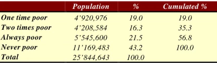
This gives a more mixed picture of poverty than static measures, and an optimistic one in the sense that a significant proportion escape poverty with only a fraction of poor staying poor year after year (out of 36.2% of poor in 1998, 25.6% remained poor and the remaining 10.6 escaped poverty). However, a less optimistic view emerges if we consider that, over the 1997-1999 period, poverty touched almost six Peruvians out of ten, that is to say more than 14 million Peruvians (table n°5).

Table n° 7-2: Poverty transitions 1997/1999

Population % Cumulated %

One time poor 4’920,976 19.0 19.0

Two times poor 4’208,584 16.3 35.3

Always poor 5’545,600 21.5 56.8

Never poor 11’169,483 43.2 100.0

Total 25’844,643 100.0

Source: Our estimation from ENAHO 1997-IV, 1998-IV and 1999-IV.

Weighted estimates

Since we know that poverty incidence increased significantly in 1999 and that it differs greatly in urban and rural areas, it is interesting to consider whether higher net poverty rates are also associated with higher transition probabilities. It is hard to say a priori whether the severely poor or the poor experience higher mobility rates. We can postulate that the extreme poor have to devote some of their resources to attenuating their higher vulnerability and, by the same token, are unable to take advantage of opportunities for upward mobility. Direct government transfers targeted may reverse this fact mostly to the extreme poor in rural areas.

A little over 40% of people in extreme poverty (who spend less than the cost of a basic food basket equivalent to the consumption of 2,318 kcal.) managed to increase their spending sufficiently to no longer suffer from extreme poverty, without being completely free from poverty nonetheless. However, nearly six « extremely poor » people out of ten remained in the same condition. As for poor who were not in extreme poverty, nearly 40% escaped from poverty whereas 20% plunged into extreme poverty. Out of the 20% of non-poor who moved into poverty, four fifths managed to maintain an overall level of spending above the cost of the basic food basket and the remaining fifth fell into extreme poverty. These results are of vital importance in assessing poverty reduction policies that attempt to give priority to targeting the « extremely poor ».

We constructed poverty lines specific to each one of the 7 geographical regions. In this way we were able to take into account absolute and relative price differences across regions and differences in consumption patterns and thus get regional comparable as well a national poverty figure. Concerning inter-temporal comparisons, we used price indexes broken down into eight sub-groups for the 24 departmental capitals in order to deflated expenditures.

It can also be observed that twice as many people fall into poverty in rural areas than in urban areas, and also that there are approximately 40% more cases of being freed of poverty in urban areas. Asset diversification strategies and targeted social expenditures are thus insufficient to reduce vulnerability in rural areas largely dependent on non-irrigated agricultural production. It should be noted that, despite lower population figures, extreme poverty is concentrated in rural areas.

8. THE STEADY STATE POVERTY RATE

The transition matrices can be used to calculate a poverty equilibrium rate (reached when flows into and out of poverty are equal). In the present case, the rate stands at 41.3%, relatively close to the rate observed in 19997_{. However, as Stevens, Bane, and Burgess and Popper in the United States and Jenkins} in the United Kingdom have remarked, the probabilities of transition are not stable over time and remain highly dependent on the households’ initial situation despite the observed mobility. Hence, examination of the transitions between 1998 and 1999 shows that the probabilities of escaping from poverty fell from 28% to 25%, whereas the probabilities of becoming poor rose from 20% to 22% (the equilibrium rate reaches 46.8%). Hence, the percentage of people escaping from poverty was slightly higher when seen from the angle of annual transitions (1997/98 and 1998/99) rather than from the period 1997/99. It therefore emerges that these two-year transition matrices cannot be extrapolated to obtain a single long-term poverty equilibrium rate.

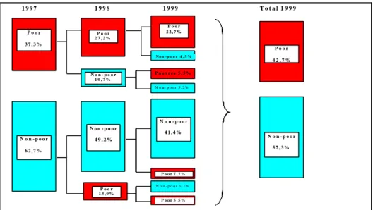
The following diagram gives an idea of the complexity of poverty transition during the three years in question. In particular, its shows that approximately half the poor people who escaped from poverty in 1997 and 1998, returned to it in 1999. Conversely, among the 13% of individual who fell into poverty in 1998, half escaped it in 1999. This reflects the vulnerability of a category of households, which is unable to escape poverty on a permanent basis, and suggests the need to reconsider the interpretation of annual transitions in poverty.

Figure n° 8-1: Flows into and out of poverty, 1997-1999

7. The steady state poverty rate can be calculate as follows: H*= Anp/ (Apn+ Anp); = 1/ ((Anp/Apn) + 1) where Anp= poverty exit rate between t y t+1

Apn= poverty entry rate between t y t+1

1 9 9 7 1 9 9 8 1 9 9 9 T o t a l 1 9 9 9 P o o r 3 7 , 3 % P o o r 2 7 , 2 % N o n - p o o r 6 2 , 7 % N o n - p o o r 4 9 , 2 % N o n - p o o r 4 1 , 4 % N o n -p o o r 4 , 5 % N o n- p o o r 5 , 2 % N o n - p o o r 1 0 , 7 % P o o r 1 3 , 0 % P o o r 5 , 5 % N o n -p o o r 6 , 7 % P o o r 4 2 , 7 % N o n - p o o r 5 7 , 3 % N a t i o n a l h o u s e h o l d s u r v e y ( 3 1 0 0 p a n e l h o u s e h o l d s ) . E N A H O 9 7 - I V , 9 8 - I V , 9 9 - IV P a u v r e s 5 , 5 % P o o r 2 2 , 7 % P o o r 7 , 7 %

9. PERMANENT AND TRANSIENT POVERTY IN PERU

The diagram above shows that nearly 23% of households experienced poverty in each of the years of the observed period. These households, that can be referred to as the hard core of « permanent poor », represent over half of the total poor observed each year, the other half being comprised of « transient poor »8

. Over the whole period, 41% of households had never experienced poverty, whereas 36% went between poverty and non-poverty. This means that poverty is a far wider-reaching phenomenon, given that six out of ten Peruvians were touched by poverty at least once during the period 1997-1999.

This mobility between poverty and non-poverty is not specific to the Peruvian population. In its latest report on poverty, the World Bank gives comparable figures for other developing countries. Transient poverty represented a share ranging from 47% of the total poor in the Ivory Coast to 85% in Zimbabwe (see table below).

Table n° 9-1: Permanent and transient poverty

Country Period

Permanent

poor Transient poor Never poor

Peru 1997-99 21.5 35.3 43.2 China 1985-90 6.2 47.8 46.0 Ivory Coast 1987-88 25.0 22.0 53.0 Ethiopia 1994-97 24.8 30.1 45.1 Pakistan 1986-91 3.0 55.3 41.7 Russian Federation 1992-93 12.6 30.2 57.2 South Africa 1993-98 22.7 31.5 45.8 Zimbabwe 1992/93-1995/96 10.6 59.6 29.8

Source: Attacking Poverty, World Bank 2000 (draft), p.21 and our estimates for Peru.

Jalan and Ravallion (1998) have recently proposed a new indicator distinguishing between chronic and temporary poverty. The chronically poor are defined as people whose long term per capita consumption (or permanent income, according to the life cycle theory concept) is below the poverty line. The difference between observed poverty and permanent poverty provides us with the transient share of poverty, a breakdown that is immediately available for additively separable indicators such as those in the FGT family. The chronic share is therefore the value of the poverty indicator when spending does not fluctuate close to its average rate over a period of time9

. Vulnerable populations suffer greater fluctuations in their income and, as they do not have sufficient savings, they pass on such shocks in their levels of spending. Hence, for example, a household may be deemed « permanently » poor over a period of 5 years although it was poor for one year only, if spending for that year was well below the poverty line and thus pulled the average spending over five years down to below the poverty line. Formally:

Git = per capita expenditure of household i in period t

Gimy= average per capita expenditure of household i over the whole period Pit = a poverty indicator for household i in period t

Permanent poverty: Ci= P(Gimy, .... Gnmy) Transient poverty:

Ti=P(Git, ... Gnt)- P(Gimy, ...Gnmy)

The aforementioned components can be gathered to obtain a national level indicator. For that it is necessary to have poverty indicators that can be additive decomposable, both in the individual and the temporal dimension (such as FGT).

A disadvantage of inter-temporal aggregation is that poverty in a future period may depend on present consumption (or poverty). This could be the case, for instance, of present consumption of durable consumer goods, which are work tools that generate income for households. This potential problem can be avoided by using an expenditure measure that takes into account the « use » value of such goods.

In their study of poverty dynamics in southern China, Jalan & Ravalllion propose the poverty gap square as the poverty indicator, in order to take into account the distance below the poverty line and to give more weight to expenditure values that are more distant from the poverty line.

Git* is the per capita household expenditures normalized by the poverty line P(Git)= (1-Git*)² if Git*<1

=0 if G*>=1

From this decomposition several poor household categories can be defined: 1) Currently poor but not permanent poor.

2) Currently poor and permanent poor. 3) Not currently poor but permanent poor.

If we take average household spending for the period 1997-99, it can be seen that 35.8% of the population was below the poverty line, i.e. a higher percentage than the number of poor individuals in each

9. A similar approach was adopted by Fields (1999) to study the relation between economic mobility and long-term inequalities. As far as equity is concerned, a society with the same degree of inequality but with greater mobility can be considered as « fairer » than another with a lesser degree of mobility.

year. In other words, around 12% of vulnerable households suffered from a drop in their spending that were sufficiently large to bring their average spending for the period 1997-99 to below the poverty line. The accent here is less on the volatility of income, as lean years can be compensated for by good years. From this angle, poverty appears to be partly a problem of uninsured or unanticipated risk. In certain cases this vulnerability can lead households into poverty traps, for instance when the children are taken out of school or when medical care is not given.

10. SENSIBILITY TO POVERTY LINE AND MEASUREMENT ERRORS

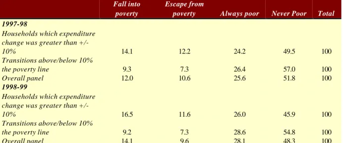
In order to test the sensitivity of our results to poverty line definitions and to expenditure measurement errors, first we considered a poverty range of 10% around the poverty line and second, took into account only transitions generated by changes in expenditure exceeding 10%. In this way it is possible to appreciate whether the observed poverty transitions are due to households very near the poverty line or to transitions implying small changes in per capita expenditure.

Table n° 10-1: Sensibility of poverty transitions to poverty line and measurement errors

Fall into poverty

Escape from

poverty Always poor Never Poor Total

1997-98

Households which expenditure change was greater than

+/-10% 14.1 12.2 24.2 49.5 100

Transitions above/below 10%

the poverty line 9.3 7.3 26.4 57.0 100

Overall panel 12.0 10.6 25.6 51.8 100

1998-99

Households which expenditure change was greater than

+/-10% 16.5 11.6 26.0 45.9 100

Transitions above/below 10%

the poverty line 9.2 7.3 28.6 54.8 100

Overall panel 14.1 9.6 28.1 48.3 100

Source: Our estimation from ENAHO 1997-IV, 1998-IV and 1999-IV. Weighted estimates

The conclusions were practically the same, indicating the fact that flows to and from poverty were relatively clear-cut. This is partly due to the fact that nearly 85% of households experienced a percentage variation in expenditure greater that 10% from one year to another, and partly that the observed variations in living standards mainly resulted from changes in the size or make-up of households, the rate of participation of their members, the dependency ratio, etc., rather than variations in the rates of remuneration on the labor market. Higher sensitivity of transitions is related to the definition of poverty lines, which results from the fact that cdf for household per capita expenditures are very steepest over the poverty line range so defined. It may be interesting to examine relative economic mobility through a quintile mobility matrix. Tables 8 and 9 show that there is an important degree of mobility among Peruvian households: no more than 50% of individuals remain in the same quintile in two consecutive years. Moreover, around 20% of the population experienced upward mobility of one-quintile in 1997/98 while those who moved downward represented 21%. Simultaneously to the increase in the poverty rate between 1998/99, less individuals (16%) moved upwards by one quintile. It can be noted from these transition matrices that most economic mobility is

relatively short-ranged. Only around 5% of individuals moved farther, either upward or downward, than one quintile in the expenditure distribution during the 1997-1999 period.

Table n° 10-2 / Table n° 10-3: Quintile transition matrix

Table n° 10-4: Transition matrix mobility indicators

1997/98 1998/99

Percentage on diagonal 48.8 50.3

Percentage that moved up by one quintile 19.6 16.0

Percentage that moved up by two or more

quintiles 5.6 4.8

Percentage that moved down by one quintile 21.0 19.7

Percentage that moved down by two or more

quintiles 5.0 5.0

Source: Our estimation from ENAHO 1997-IV and 1998-IV. Weighted estimates

11. PROFILE OF POVERTY TRANSITIONS

In the same way, it is possible to compile static poverty profiles, showing the incidence of poverty according to households’ demographical and economic characteristics and also to build a profile of the vulnerable population (i.e. people who fall into or escape poverty), the chronically poor and those that are never in a state of poverty. Of course, this exercise particularly serves to characterize these different populations and not to establish relations of causality between the population’s characteristics and the different poverty transitions (these are, to a certain extent, unconditional risks). The concomitant effects of the different variables will be examined later, in the presentation of the main results of the econometric estimates.

These profiles provide an outline of typical households. For instance, the profile of households in a state of permanent poverty corresponds to a relatively large household with a low number of working members and hence a quite high dependency level. The head of household lives in the sierra, is of average age, cohabits and has not received an education (on a national level, only 8% of heads of households have not been to school whereas the figure reaches 20% amongst the chronically poor). Vulnerable households are

1999 quintile 1998 quintile I II III IV V I 13.68 5.04 0.85 0.39 0.05 II 4.97 7.54 5.19 2.10 0.21 III 0.92 5.40 7.32 5.11 1.24 IV 0.41 1.59 5.04 8.10 4.84 V 0.04 0.41 1.61 4.28 13.65 1998 quintile 1997 quintile I II III IV V I 13.15 5.22 1.22 0.32 0.11 II 5.18 8.26 4.41 1.85 0.30 III 1.38 4.74 6.95 5.15 1.77 IV 0.32 1.40 5.96 7.51 4.79 V 0.07 0.44 1.40 5.15 12.94

characterized by the young age of their head, by living in a rural area and by only having reached a primary level of education. The benefit of a secondary education prevents people from becoming chronically poor but is not sufficient to allow them to avoid episodes of poverty. A particularly significant fact is that there does not seem to be any relationship between the risk of poverty and the fact that the head of household is a woman. On the contrary, a higher percentage of such households manage to escape from poverty than for households where the head is a man. Households that are sheltered from poverty are households residing in the large coastal cities, with a less than average size, a high rate of participation in the labor market and whose heads are employers or salaried executives with a higher level of education (see table in appendix).

12. POVERTY AND INEQUALITY DECOMPOSITIONS

In the past three years Peruvian growth performance has been very poor. Household per capita expenditures declined by 12,2% between 1997 and 1999 and the poverty rate increased, as we have seen, from 36.2% to 42.1%. In this section we address the question of the extent to which this change in poverty rates is due to pure growth effects or to changes in inequality, or to put it other way, to what extent the recent growth performance has been pro-poor? In answering these questions we will limit our decomposition to poverty incidence (Po) following recent work by Mahmoudi who provides an exact decomposition, contrarily to pioneering work by Datt and Ravallion. We will only consider households in the panel in order to avoid de effects of varying sample size and to ensure comparability with the decomposition proposed by Fields and presented in the next section.

According to the approach developed by Datt and Ravallion, poverty changes can be decomposed into one part due to growth, another due to changes in inequality and a third component identified as a residual. Of course, there is no reason for the growth and inequality components to vary in the same direction. To carry out the decomposition, Datt and Ravallion focus on poverty indicators that can be represented in terms of poverty line (z), mean expenditures (µt) and the Lorenz curve (Lt), (which indicates inequality

among individuals):

Pt = P(z/µt, Lt)

The general principle upon which Datt and Ravallion bases their decomposition consist in considering the growth component as the poverty change that result of a change in mean expenditure (µ), holding constant the Lorenz curve (Lr) and given the poverty line. The redistribution component is equal to the poverty change due to changes in the Lorenz curve, holding constant average expenditure.

Pt+n - Pt = [P(z/µt+n, Lt) - P(z/µt, Lt)] + [P(z/µt, Lt+n) – P(z/µt, Lt)] + residual P_µ Growth contribution Pψ Redistribution contribution

According to Datt and Ravallion, the residual appears «whenever the poverty measure is not additively separable between (µ) and L, i.e. whenever the marginal effects on the poverty index of changes in the mean (Lorenz curve) depend on the precise Lorenz curve (mean) » (Ravallion, Datt 1991:4).

The method proposed by Datt and Ravallion implies the econometric estimation of a Lorenz curve. The form of the function estimated by the authors is « elliptical » (or a general quadratic function). This regression is estimated by OLS with the variables expressed in logarithms. Chen, Datt and Ravallion provide software (POVCAL) designed to estimate the parameters of the Lorenz function when expenditure data is grouped.

According to McCulloch y Baulch (1998:4), the residual appears as a result of the choice of the reference period and is equal to the difference between the growth components measured at the final and initial distributions. They note that this residual is neither an econometric residual nor is it related to the quality of the data.

Mahmoudi for whom the existence of a residual is an undesirable characteristic of the method due to misspecification has criticized this interpretation of the residual. “The residual in Datt-Ravallion’s method show the inability of the method to separate pure growth and redistribution components completely and ignore all possibility of decomposition in a unique formula, which makes it sensitive to the choice of distribution as the reference” (Mahmoudi, 1998:3).

The alternative method suggested by Mahmoudi relies on the relationship between the cumulative density function (cdf) of expenditure and the Lorenz curve. Mahmoudi underlines that the cdf function can be used to highlight the redistribution effect since the Lorenz curve is non other than the integral (normalized by the mean) of the distribution function. It allows for an exact decomposition of poverty changes in a pure growth effect and a redistribution effect and has the advantage of not requiring a parametric estimation of Lorenz curves.

L(p) = 1/µ

∫

ρ

0

cdf -1 (π) dπ

Since it is postulated that cdf1 and cdf2 have, by construction, the same mean value, then Mahmoudi shows that:

µ [L2(p) – L1(p) ] =

∫

ρ

0

[ cdf2-1 (π) - cdf1–1 (π) ] dπ

The change in the headcount poverty ratio that can be attributed to growth can be expressed as: Pt+n - Pt = [P(cdf2, z) – P(cdf1, z) ] = cdf1(zµt /µt+n) - cdf1(z)

Thus, the method consists in constructing a new distribution-scaling up (by average change in expenditure) the reference distribution so it is homothetically shifted. We then compare this distribution in which all expenditures has been increased by the average growth with the observed distribution in the final period. The differences in poverty rates are naturally due to the redistribution effect whereas the difference between the reference distribution and the simulated distribution yields the growth contribution to poverty changes. There is no residual from this decomposition but, naturally, the growth and redistribution components will vary according to which distribution is taken as the reference distribution. Mahmoudi proposes simply to take the average of each component obtained by considering the first and then the second distribution as

the reference (in the first case the distribution is scaled up, whereas in the second it is scaled down, if growth is positive between the two periods).

If we wish to compare the growth contribution (or the redistribution effect) considering two periods of different lengths (for instance 1980-85 and 1985-2000), it is convenient to normalize the redistribution component using the absolute value of the growth component as denominator, as was suggested by McCulloch y Baulch.

Anti-poor bias of growth = - ∆Pψ /∆Pµ

The table below shows the results obtained by applying this methodology to the Peruvian case. Only headcount poverty change decomposition is reported. First, it should be recalled that inequality, measured in terms of real expenditure (at 1999 prices, deflated by disaggregated price index for 8 subgroups for each of the 24 departamentos’ capital and weighted at the individual level), diminished during the period considered (1997-1999). It passed from 0.482 in 1997 to 0.475 in 1998 and diminished further to 0.467 in 1999, although a contrasted evolution was observed in urban and rural areas. While inequality diminished steadily, though by small proportions, in urban areas it first increased and then decreased by 6% between 1998 and 1999 in rural areas. It can also be observed that poverty headcount increased most in urban areas (almost 6% points) whereas in rural areas the increase in poverty rates was moderate (less than 2% points). We can therefore expect a bigger growth effect in urban areas than in rural areas and inversely with respect to the redistribution effect.

Table n° 12-1: Decomposition of poverty changes into growth and inequality effects Peru 1997-1999

Average of reference periods to and T1

National Urban Rural

97/98 98/99 97/99 97/99 97/99

Growth effect 3.12 4.53 7.74 9.23 -0.02

Redistribution effect -1.68 -0.03 -1.80 -1.03 1.72

Total poverty change 1.44 4.5 5.94 8.2 1.70

Pro poor growth bias 0.54 0.01 0.23 0.11 86.0

Source: our estimation from ENAHO 1997, 1998 and 1999 surveys. Panel households Note: Poverty incidence (Po) at the (weighted) individual level.

It is interesting to note that, at that national level over the period 1997-99, the decrease in mean household expenditure accounts for all the increase in poverty incidence; the redistribution effect moved in the opposite direction, contributing to diminish the poverty rate that would otherwise have been even higher. Redistribution effects reduced the poverty headcount by 2 percentage points, whereas falling mean household expenditure raised poverty incidence by almost 8 percentage points between 1997 and 1999. However, quite different pictures appear when we consider the sub periods 1997/98 and 1998/99 and when we distinguish between rural and urban areas. Huge adverse growth effects were partly mitigated by redistribution effects in urban areas, while small positive growth effects were overridden by negative distributive effects in rural areas (see table above). The first recession year (1997/98) was characterized by an important redistribution of household expenditure that halved poverty increase due to poor growth performance. The second recession year (1998/99), although it implied a reduction in mean household expenditures similar to that recorded in 1997/98, had lower favorable distributional changes. The normalized pro poor bias was significant in 1997/1998; decline in growth was not biased against the poor since the actual increase in poverty was less than what would occur with distributionally neutral growth (the headcount is more than 50% lower than it would otherwise have been). In 1998/99 the pro poor bias practically disappeared. It would be tempting to interpret this neutrality of recession as reflecting the failure of public policy in favor of the poor. However, a more rigorous analysis based on panel data is needed before drawing such conclusions (see below). It is worth noting that in rural areas growth was biased against the poor, accounting for almost all the poverty increase, while in urban areas it was biased in favor of the poor, though in a modest proportion (11%).

13. INEQUALITY DECOMPOSITION BETWEEN AND WITHIN GROUPS

Next, we examined the sources of economic heterogeneity by decomposing the (Theil) inequality index between groups and within groups for both 1997 and 1998 household per capita expenditures.

The Theil inequality index can be additively decomposed between groups and within groups in the following way:

T= Σ Yi/Y ln (Yi)/(Y/N) =

Σ Yj/Y Tj + Σ Yj/Y ln (Yj/Nj)/(Y/N)

Within groups between groups

We considered geographical domains and characteristics for household heads in order to shed some light on the nature of inequality and its evolution. Despite the huge gap in living standards between rural and urban areas, only about 25% of total inequality was accounted for by differences in their average expenditures. There is no sign either that it is increasing (it actually fell slightly). Considering inter-regional differences (for INEI’s seven geographical regions) indicated that they accounted for around one third of total inequality and that the gap was reduced as urban regions were more heavily exposed to deteriorating living conditions than rural regions. Interestingly enough, the sex of household heads did not contribute in any significant way to total inequality, similarly to household age group or its civil status. In contrast to this, the level of education of household heads is by and large the major single household characteristic contributing to overall inequality (36% in 1997). It can be noted that its relative (as well absolute) contribution fell by around 10 percentage points between 1997 and 1998, suggesting an important reduction in the economic benefits to education. Finally and not surprisingly, workers’ activity had a small impact since unemployment and inactivity concern a very small number of household heads.

Table n° 13-1: Theil inequality between groups, level and % of total inequality

1997 1998 1997 1998

Level Between group as % of total

Geographical domain 0.16505 0.13766 36.4% 32.7%

Rural/ urban area 0.11436 0.10146 25.2% 24.1%

Sex 0.00023 0.00269 0.1% 0.6%

Age group 0.0122 0.00684 2.7% 1.6%

Education level 0.1639 0.11291 36.1% 26.7%

Activity 0.01881 0.01677 4.1% 4.0%

Civil status 0.02296 0.02065 5.1% 4.9%

Source: our estimation from ENAHO 1997, 1998 and 1999 surveys. Panel households

14. DECOMPOSING INCOME MOBILITY IN PANEL DATA: FIELDS/OK’S GROWTH AND “EXCHANGE” MOBILITY

A new generation of mobility indicators has been proposed by Fields & Ok, based on an axiomatic approach inspired by Shorroks’ work (1978) and the Markandya mobility indicator (1984). The proposed indicators have the particularity of allowing a distinction to be made between the two aspects of mobility (structural and exchange mobility) and of not requiring the independence hypothesis of a first order Markovian process.

The symmetric economic mobility indicator proposed by Fields (1998) and Fields & Ok (1996, 1999) serves to measure the importance of flows implied by expenditure mobility. The indicator is based on changes in expenditure level. In order to take into account the fact that a transferred amount does not have the same significance for low and high incomes, the authors propose that the logarithm of income should be considered. In this way, an equal transfer of expenditure will have a greater importance for poor households than for wealthier households.

Being:

xi household ( i ) per capita expenditure in the initial year yi household ( i ) per capita expenditure in the final year dn (x, y) = Σ |xi-yi|

dn (x, y) measures the total amount of change in expenditure between the initial and the final observation period and is equal to total mobility. Fields & Ok proposes that this flow be expressed in per capita terms and as percentages of the average of base-year income. In this way, mobility can be referred to an order of magnitude relevant for the analysis.

mn (x, y) = 1/n Σ |xi-yi| pn (x, y) = Σ |xi-yi| / Σ xi

mn (x, y) is the average total mobility per household and pn (x, y) is the total mobility in percentage of total expenditure in the initial year. All variables are expressed in logarithms.

An important feature of the Fields & Ok index is that it can be decomposed into two parts: the first measures the mobility due to growth (or decrease in growth) and the second measures the mobility due to the changes in position in the expenditure scale, with constant average expenditure. Thus, when the economy grows, the decomposition of dn in the two components is given by:

dn (x, y) = Gn (x, y) + Tn (x, y)

The mobility due to growth is the mobility that will have occur if all household expenditures had grown in the same proportions and it is equal to:

Gn (x, y) = Σ yi - Σ xi

While the mobility due to transfers between households is the mobility that would have occurred if the households had changed their position in the distribution, maintaining constant aggregate expenditure. It is given by:

Tn (x, y) = 2 (iε Ln(xy) Σ (xi -yi ))

Ln(xy) Is the group of households that suffered a diminution in their spending. To summarize, total mobility in the growth phase is decomposed as follows: dn (x, y) = Σ |xi-yi| = Σ yi - Σ xi + 2 (iε Ln(xy) Σ (xi -yi ))

and in a recession phase the index is as follow:

dn (x, y) = Σ |xi-yi| = Σ xi - Σ yi + 2 (iε Wn(xy) Σ (xi -yi ))

Wn(xy) is the group of households that had an increase in their expenditures.

The non-directional or symmetric index of expenditure mobility is interesting insofar as it informs us about the degree of instability that exists in income distribution or household spending. A difficulty that could appear is the sensitivity of this index to extreme values, which renders average values representative of changes in the distribution of household expenditures. This can be overcome, as proposed by Fields (1998), by examining the whole cumulative distribution of expenditure changes and performing a first order dominance test.

15. DIRECTIONAL MOBILITY INDEX

The directional mobility index consists in examining the stochastic dominance of the distribution of changes in household expenditure levels between two different years. This approach allows for inter-temporary comparisons of welfare (Fields, Leary, Ok, 1998:2).

It is important to insist on the fact that the Fields & Ok index does not depend on the first order Markovian process hypothesis, implicit in annual transition matrixes, which is rejected in most empirical mobility studies. They are also the only ones to register mobility when the spending of all households grows homothetically (Fields, 1998:6).

Economic mobility can be measured without introducing the discontinuities that occur when populations are divided into categories of poor and non-poor, or accepting the independence hypothesis of first order Markovian processes. This is the case for the economic mobility indicator proposed by Fields and Ok (Fields, 1998 and Fields & Ok, 1996). It enables a distinction to be made between growth-related

structural mobility and so-called « exchange » mobility, and measures the importance of transfers of mobility-related flows of expenditure. Growth mobility is the mobility that would have occurred if all household expenditure had varied in the same proportions, whereas exchange mobility is the mobility that occurs when households change their position in the distribution.

The calculations made for Peru show that total mobility was quite considerable during the period from 1997-1999, as it represented approximately 40% of average per capita expenditure. More interestingly, exchange mobility accounted for over two-thirds of total mobility, and also fell (from 90% to 86% of total mobility in the sub periods 97/98 and 98/99) together with total mobility when the average expenditure level fell.

Table n° 15-1: Fields/Ok income mobility index (En % household per capita expenditure)

Total Growth Exchange

97/98 42.48 4.06 38.42 100% 10% 90% 98/99 37.38 5.26 32.12 100% 14% 86% 97/99 45.12 9.16 35.96 100% 20% 80%

Source: our estimation from ENAHO 1997, 1998 and 1999 surveys. Figure n° 15-1: Directional and absolute mobility

16. MODELLING POVERTY TRANSITIONS

In commenting the poverty transition profile, we have so far examined the unconditional risk that households of given characteristics may experience any of the poverty transition states. This has allowed identifying some variables that may be relevant for policy making. For more analytical purposes though we need to consider the relative risks conditional on the other factors that determines poverty transitions. We will particularly focus on the factors that enable households to escape poverty since this may give some clues for improving anti-poverty policies.

Movilidad direccional 1997/98 y 1998/99

% de la poblacion

diferencia de logs del gasto

-1.25 -1 -.5 0 .5 1 1.25 1 25 50 75 100 Movilidad absoluta 1997/98 y 1998/99 % de la poblacion

valor abs de diferencia de logs

0 .25 .5 .75 1 1.25 1.5 1 25 50 75 100

As is well known, static, cross-section econometric models allows us only to identify the correlates of poverty, that is to say characteristics linked to poverty but in no case can be inferred causality patterns from this kind of analysis. This can only be done in the context of panel data by modeling the factors associated with poverty transitions. This is the first step in understanding poverty causality (or better triggering factors). However, we must be very cautious in deducing from our results policy oriented recommendations for this is essentially a partial equilibrium approach and we need to understand also the indirect effects. For instance, it is not because we may find a strong positive relationship between the probability of escaping poverty and labor market participation of secondary household members that it follows that a nation-wide increase in labor force participation rates will reduce poverty. This will also depend on how the labor market will react to the increase in the labor supply and it is by no means guaranteed that all workers will be better off. We must not ignore either that it may be very difficult to consider only exogenous variables among the explanatory variables. Most variables used in regressions have a two-way causality, including household demographic characteristics. More educated urban households, which are also richer than less educated rural households, may decide no to have as many children as do rural households. Each child adds to the denominator of income per capita but not to the numerator, so it is- at least in the short run- an automatic decline in welfare. We can argue that household and individual characteristics are fixed in the short run but are endogenous in the medium and the long run. Our three years (1997-1999) panel allows us to consider events or shocks that are not contemporaneous to the poverty transitions, limiting somewhat the problem of simultaneity and of endogenous variables. We attempted to estimate the determining factors of the different forms of poverty transition between 1998 and 1999 using a multinomial logit model since our dependent variable is a categorical variable with four values corresponding to each of the poverty transitions in our matrix (chronic poverty, falling into poverty, escaping from poverty and never in poverty). We can postulate that there is a latent unobserved variable y* related to the “capacity of households to protect themselves against poverty or escape it”. If this is the case (an hypothesis that is known as the parallel regression hypothesis which can be tested10

) the appropriated model is the ordered multinomial logit. If this hypothesis is not granted, then we need to estimate an unordered multinomial model. The choice of the logit function is justified by the simplicity in interpreting the results in terms of odds ratio or relative risk ratios. In the ordered model we have only one set of parameters estimated whereas in the unordered model each poverty transition state has its own parameters (with one state as base case). From this framework we will attempt to answer to various questions. Do the factors explaining chronic poverty equally important in explaining entries in poverty? Are there specific events linked to escaping poverty, different from those explaining the probability of being never poor? What role is played by geographical variables in poverty transitions?

10. The parallel regression or the proportional-odds hypothesis can be tested ruining an unconstrained and a constrained regression in which it is imposed the restriction that the coefficients are equal across categories and then performing an approximate likelihood-ratio test (see STATA manual). If we estimate an unordered multinomial model when the dependent variable is ordered, then there is efficiency loose since we are not using all the information available. Inversely, if the dependent variable in not ordered and we estimate an ordered model, then our estimates will be biased or even nonsensical. A significant p-value is evidence to reject the null hypothesis that the coefficients are equal across categories (Scott, 1997:149)