The Formation of Risk Sharing Networks

(1)

DIAL • 4, rue d’Enghien • 75010 Paris • Téléphone (33) 01 53 24 14 50 • Fax (33) 01 53 24 14 51 E-mail : dial@dial.prd.fr • Site : www.dial.prd.fr

D

OCUMENT DE

T

RAVAIL

DT/2005-13

The Formation of Risk Sharing

Networks

Marcel FAFCHAMPS

Flore GUBERT

(2)

THE FORMATION OF RISK SHARING NETWORKS

1 Marcel Fafchamps University of Oxford Department of Economics marcel.fafchamps@economics.ox.ac.uk Flore Gubert IRD-Paris, DIAL gubert@dial.prd.fr

Document de travail DIAL

Novembre 2005

ABSTRACT

This paper examines the endogenous formation of risk sharing networks in the rural Philippines. We show that geographic proximity is a major determinant of interpersonal relationships. We find little evidence that people form relationships to pool income risk. The existence of a pre-existing relationship between two individuals is a major determinant of subsequent gifts and informal loans between them, controlling for other proximity factors. From this we conclude that these transfers and informal loans are embedded in interpersonal relationships. These relationships are largely determined by proximity factors and are only weakly the result of purposeful diversification of income risk. There is, however, some evidence that the formation of risk sharing links is aimed at pooling health risk. The paper also makes a methodological contribution to the estimation of dyadic models.

Keywords: Network, risk-sharing, dyadic model, Philippines

RESUMÉ

Cet article examine la façon dont se forment les réseaux informels de partage des risques à partir de données collectées aux Philippines. Nous trouvons que les ménages enquêtés choisissent des partenaires potentiels d'entraide géographiquement proches d'eux mais non économiquement distants d'eux. Nous trouvons également que l'existence d'un lien ex ante est un déterminant important des dons et prêts informels observés entre ménages. Nous concluons de ces résultats empiriques que les transactions observées entre ménages s'inscrivent dans le cadre de relations de voisinage dont l'objectif premier n'est pas la diversification des risques de revenu. En revanche, un partage des risques liés à la santé semble être à l'oeuvre. L'article fait une contribution méthodologique à travers l'estimation de modèles dyadiques.

Mots clés : Réseau, partage du risque, modèle dyadique, Philippines JEL Code : D85, O12, C49

(3)

List of tables

Table 1: Descriptive statistics on household... 31

Table 2: Relationship of insurance partners to household head... 32

Table 3: Residence of insurance partner... 33

Table 4: Variables used in the regressions... 34

Table 5: Network links ... 35

Table 6: Testing symmetry of determinants of network links ... 36

Table 7: Network links with level effects ... 37

Table 8: Network links controlling for self-selection ... 38

Table 9: Gift and network link... 39

List of appendices

Appendix 1: Wealth instrumenting equation ... 41

(4)

1. Introduction

In an in‡uential paper, Granovetter (1985) argued that market transactions should not be viewed as anonymous and impersonal but as embedded in a web of inter-personal relationships. Gra-novetter based his conclusion upon years of research on labor markets and business relationships in the US. Granovetter (1995) showed, for instance, that most jobs are obtained through some kind of referral process, the reliability of which is often based on prior acquaintance. Following Granovetter’s work, many researchers in economics and other social sciences have documented the importance of relational contracting (e.g. Bernstein 1992, Bernstein 1996, Johnson, McMil-lan & Woodru¤ 2002) and the role that networks of interpersonal relationships play in the circulation of information (e.g. Barr 2000, Foster & Rosenzweig 1995, Romani 2003, Bandiera & Rasul 2002). Fafchamps (2004) and Fisman (2003) have shown that prior acquaintance plays a paramount role in market exchange in African manufacturing because it forms the basis for trust. The importance of personal relationships has also been documented in agricultural trade (e.g. Meillassoux 1971, Shapiro 1979, Fafchamps & Minten 1999, Fafchamps & Minten 2002). The purpose of this paper is to investigate the e¤ect of interpersonal relationships on economic transactions.

Much theoretical work has been done on networks by sociologists who have started thinking about networks as early as the 1960’s (Mitchell 1969) and modeling them using graph theory (e.g. Raub & Weesie 1990, Weesie & Raub 2000). More recently, networks have begun receiving attention from economic theorists. Bala & Goyal (2000) and Goyal, van der Leij & Moraga-Gonzalez (2004), for instance, have studied the relationship between network architecture and underlying incentives. Kranton & Minehart (2001) have examined the restrictions on exchange that network relationships place on exchange. Genicot & Ray (2003) and Bloch, Genicot & Ray (2004) investigate the conditions under which speci…c network architectures are stable with

(5)

respect to individual and group deviations. Recent progress has also been made –primarily by epidemiologists or under their impetus –in the modeling of large networks (Vega-Redondo 2004). Development economists have long suspected that interpersonal relationships help shape economic exchange and agrarian institutions (e.g. Basu 1986, Bardhan 1984). This is probably because formal institutions often are weak and must be supplemented by interpersonal trust (Fafchamps 2005). This appears particularly true for risk sharing which, in addition to self-insurance via precautionary saving, has been shown to be a fundamental risk coping mechanism for the rural poor (e.g. Rosenzweig & Wolpin 1988, Townsend 1994, Ligon, Thomas & Worrall 2001, Ligon, Thomas & Worrall 2000, Fafchamps 2003). The pooling of idiosyncratic risk remains primarily informal in much of the developing world (e.g. Fafchamps 1992, Coate & Ravallion 1993, Foster & Rosenzweig 2001). In addition to risk sharing within households (e.g. Rosenzweig & Stark 1989, Dercon & Krishnan 2000), transfers and inter-personal loans constitute primary channels of risk pooling (Udry 1994). Transfers and interpersonal loans have been shown to travel primarily along long-lasting interpersonal networks (e.g. Ellsworth 1989, Lucas & Stark 1985). The same is true of labor exchange arrangements (Krishnan & Sciubba 2004).

In this paper we study the e¤ect of pre-existing relationships on subsequent gifts and trans-fers, controlling for shared characteristics. Our empirical investigation is based on survey data collected in rural Philippines for the purpose of studying risk sharing. Using these data, Fafchamps & Lund (2003) have indeed shown that informal gifts and loans serve a risk sharing purpose but also that the extent of risk sharing appears limited by the extent of interpersonal networks. Here we examine the factors determining the formation of risk sharing network and the extent to which these networks de facto shape subsequent gifts and loans.

We show that geographic proximity is a major determinant of interpersonal relationships. We only …nd weak evidence that people form such relationships to explicitly diversify risk and

(6)

maximize gains from risk pooling. The existence of a pre-existing relationship between two indi-viduals is a major determinant of subsequent gifts and informal loans between them, controlling for other proximity factors. From this we conclude that these transfers and informal loans are embedded in interpersonal relationships. These relationships are largely determined by proxim-ity factors and are only weakly the result of purposeful diversi…cation of income risk. There is, however, some evidence that in the study area the formation of risk sharing links is aimed at pooling health risk.

The paper is organized as follows. We begin by developing a simple model of the formation of risk sharing arrangements between pairs of agents. We use it to derive testable hypotheses that are suited to the data at hand. Econometric issues are discussed in Section 3. In Section 4 we present the data and its main characteristics. Econometric results are discussed in detail in Section 5.

2. Conceptual framework

To motivate the empirical analysis, we begin by constructing a simple model of relationship formation. Consider two individuals i and j. The cost to i of establishing a relationship with j increases with the distance dij between i and j:

Ci = C(dij) (2.1)

We interpret distance as a K-dimensional vector dij = fd1ij; :::; dKijg that includes dimensions such as spatial distance, family relatedness, shared activities and religion, similar age and gender, etc. The idea is that it is easier to establish –and maintain –a relationship with people who are close in some important respect. We thus assume that C0 _{0 for all d}k

(7)

wish to investigate econometrically.

A relationship with j generates bene…ts Bi to i.1 We assume that bene…ts depend on the distance between i and j:

Bi= B(dij; Lij) (2.2)

where Lij = 1 if there is a link between them, and zero otherwise. If a link is bene…cial, we have B(dij; 1) > B(dij; 0) for all dij. If a link is essential for any bene…t to be achieved, then B(dij; 0) = 0 for all dij.

In many economic situations of interest, gains from trade are largest between economic agents with di¤erent endowments. It is therefore reasonable to assume that the bene…t derived from a link increase with distance, i.e., that

@(B(dij; 1) B(dij; 0))

@dk_ij > 0 for k 2 G K

One possible example that we investigate in the empirical section is mutual insurance: gains from risk pooling between two individuals i and j are higher the less (positively) correlated the incomes of i and j are. For this reason, we expect mutual gains from risk sharing to be lower if both individuals have the same occupation. We also note that sensitivity to health shocks depends, among other things, on age and gender: two individuals of the same age and gender are more likely to be a¤ected by similar illnesses than individuals who di¤er a lot. As a result, the pooling of health risk should be more e¤ective between individuals that are least similar. Provided suitable data are available, these issues can be investigated directly by estimating equation (2.2) to ascertain whether the bene…t from a link indeed increases with distance.

We are also interested in endogenous network formation. We observe that, other things being

(8)

equal, it is in the interest of individual i to incur the cost of establishing a link Lij with j if:

G(dij) B(dij; 1) B(dij; 0) C(dij) > 0 (2.3)

We thus have Lij = 1 if G(dij) 0 and Lij = 0 otherwise. Factors that raise G thus make it more likely that G 0 and thus that a link is formed. It follows that, other things being equal, if @G(dij)=@dkij > 0, then an increase in distance dkij makes it more likely that Lij = 1. Since we have assume that both costs and bene…ts increase with distance, whether @G(dij)=@dkij > 0 depends on the relative speed with which costs and bene…ts increase with distance. If, for instance, C(dij) rises less rapidly with dkij than B(dij; 1) B(dij; 0), then @G(dij)=@dkij > 0 and links are more likely to be formed between distant individuals than between proximate individuals. The reverse is also true: if C(dij) rises more rapidly with dkij than B(dij; 1) B(dij; 0), then we obtain assortative matching: links are more likely to be formed between proximate individuals than between distant individuals.

In practice, choices are also a¤ected by random unobservable factors, say eij. Adding a random component to inequality (2.3) yields a dichotomous regression model of the form:

Lij = 1 if G(dij) + eij > 0

= 0 otherwise (2.4)

Coupled with a distributional assumption regarding eij and a functional form for B(:) and C(:), model (2.4) can be estimated using logit or probit. If we …nd that Pr(Lij = 1) decreases with dk_ij, this suggests that the cost of establishing a link increases more rapidly with dk_ij than the bene…t of such link.2

2

This arises a fortiori when the gain from a network link does not increase with dkij– or even falls with d k ij.

(9)

Estimating both models (2.2) and (2.4) generates important insights regarding the con-straints on economic exchange that are imposed by the cost of network formation. To illustrate this, suppose that we …nd from estimating equation (2.2) that the bene…t of a link increases with distance dk_ij. This means that larger gains from trade are achieved with more distant people – with distance measured using metric dk_ij. The question then is, are these gains from trade achieved? Suppose we …nd instead that proximate individuals are more likely to be linked. This indicates that di¢ culties in establishing trade links between people preclude the most bene…cial trade. Assortative matching driven by network costs results in sub-optimal trade patterns. The purpose of the remainder of this paper is to test this idea formally.

3. Econometric issues

Regression models (2.2) and (2.4) are both of the form:

Yij = + Xij+ uij (3.1)

where i and j are individuals, Yij is an N N matrix, and Xij is a series of N N matrices. Network analysis naturally leads to regression models of this form. The estimation of dyadic regressions such as (3.1) raises two types of di¢ culties: identi…cation; and inference. The …rst problem relates to the form in which regressors Xij enter the regression. The second relates to the estimation of standard errors.

3.1. Identi…cation

Dyadic data contains two types of information: attributes dij of the link between i and j, such as the geographical distance between them, and attributes zi and zj of the nodes i and j. The acceptable form in which regressors enter dyadic regressions depends on two criteria: whether the

(10)

dyadic relationship is symmetrical or not; and whether each individual i has the same number of links ni –or degree. We discuss these in turn.

A dyadic relationship is symmetrical if Yji = Yij for all i; j. In this case, identi…cation requires that regressors satisfy Xij = Xji. One easy way of satisfying this requirement is to specify the regression as:

Yij = + 1jzi zjj + 2(zi+ zj) + jdijj + uij (3.2)

where zi and zj are characteristics of individual i and j thought to in‡uence the likelihood of a link Yij between them. A dyadic relationship can also be directional, in which case Yij need not equal Yji. In this case, regressors need not satisfy Xij = Xji and it is possible to estimate models of the form Yij = + 1zi+ 2zj+ uij or, equivalently:

Yij = + 1(zi zj) + 2(zi+ zj) + dij+ uij (3.3)

Identi…cation is also in‡uenced by degree distribution. If all individuals have the same degree, we cannot identify ₂. This follows from the fact that dyadic observations are not independent. Consequently the joint likelihood of the sample does not decompose into a product of single observation likelihoods. When all individuals have the same degree, the structure of the joint likelihood is such that only the e¤ect of di¤erences between observations can be identi…ed. Showing this formally is beyond the scope of this paper but to see this intuitively, imagine we have data on monogamous couples and that zi denotes education. By design, all individuals are paired with one and only one other individual, irrespective of their education level. We can ask the data whether educated people marry each other, but not whether educated people are more likely to be married. This means that we can identify whether di¤erences in attributes zi zj

(11)

a¤ect the likelihood of a link, but not whether better educated people have on average more links. It follows that the e¤ect of zi+ zj cannot be estimated: we can identify 1 but not 2. Identi…cation of ₂ requires that individuals have di¤erent degrees, as would be the case, for instance, if the data included unmarried individuals or polygamous couples. Only then could we ask the data whether educated people are more likely to be married. Degree variation is thus necessary to identify level e¤ects ₂.

3.2. Standard errors

In network analysis, dyadic observations are typically not independent. This is due to the presence of individual-speci…c factors common to all observations involving this individual. It is in general reasonable to assume that E[uij; uik] 6= 0 for all k and E[uij; ukj] 6= 0 for all k. By the same reasoning, we also have E[uij; ujk] 6= 0 and E[uij; uki] 6= 0.3 Provided that regressors are exogenous, applying OLS to (3.2) and (3.3) yields consistent coe¢ cient estimates but standard errors are inconsistent, leading to incorrect inference.

Robust standard errors must correct for four-way clustering along the columns and the rows of uij. To obtain such robust standard errors, we apply the method developed by Conley (1999) to deal with spatial correlation of errors.4 Conley’s method is an extension of the robust covariance matrix popularized by White and extended to time series by Newey and West. Applied to network data, the method allows for arbitrary cross-observation correlation in the error terms involving similar individuals. The only structure imposed on the covariance structure is that

3_{This situation bears some formal resemblance to random e¤ects models with two-way error components}

discussed for instance by Baltagi (1995).

4_{Other methods have been devised to conduct inference on network data. One such method relies on}

permu-tation methods popularized by Good (2000). This method was …rst applied to network analysis by Hubert & Schultz (1976) and subsequently re…ned by Krackhardt (1987) and Nyblom, Borgatti, Roslakka & Salo (2003). Instead of correcting standard errors, permutation methods correct p-values directly. This procedure is known as Quadratic Assignment Procedure or QAP in the literature (Hubert & Schultz 1976). This approach has gained much popularity among sociologists who typically compute QAP p-values using a linear probability model. We believe our method to be statistically more e¢ cient since it does not rely on bootstrapping.

(12)

E[uij; uik] 6= 0, E[uij; ukj] 6= 0; E[uij; ujk] 6= 0 and E[uij; uki] 6= 0 for all k but E[uij; ukm] = 0 if i 6= j 6= k 6= m.

Monte Carlo simulations suggest that the standard error correction can be very sizeable in the case of network data. The bias is particularly large when the average degree is high. The correction of standard errors is essential when estimating dyadic regressions. In our case, the magnitude of the correction turns out to be relatively small because the average degree is quite low.

4. The data

Having presented the conceptual framework and discussed econometric issues, we now describe the data. A survey was conducted in four villages in the Cordillera mountains of northern Philippines between July, 1994 and March, 1995 (Lund 1996). A random sample of 206 rural household was drawn after taking a census of all households in selected rural districts. These households are dispersed over a wide area; most can only be reached by foot. Three interviews were conducted with each household at three month intervals between July 1994, just after the annual rice harvest, and March 1995, after the new rice crop had been transplanted.

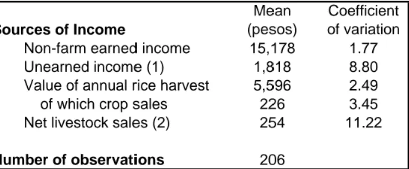
As shown in Table 1, sample households derive most of their income from non-farm activities. There are many skilled artisans in this area, and their wood carvings, woven blankets, and rattan baskets supply a growing tourist and export trade. Unearned income –mostly land rentals –is not negligible but very unevenly distributed across households, as is often the case with asset income. Although nearly all households operate their own farm, the majority do not produce enough grain to meet annual consumption needs. Sales of crops and livestock account for a minute fraction of total income. The data indicate that di¤erences in income per capita across households are signi…cantly correlated with di¤erences in wealth ( = 0:16; p-value= 0:000) and

(13)

education levels ( = 0:19; p-value= 0:000). They are also negatively correlated with di¤erences in distance from the road. This means that individuals located close to each other tend, on average, to have less similar incomes. The e¤ect is quite small, however ( = 0:05). We also …nd that households with di¤erent levels of education are less likely to be engaged in the same occupation.

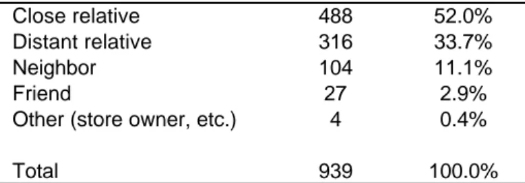
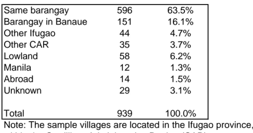
At the beginning of the survey, each household was asked to identify a number of individuals on which it could rely in case of need or to whom the respondent gives help when called upon to do so. Respondents listed on average 4.6 individuals, with a minimum of 1 and a maximum of 8. These individuals constitute what we call the network of insurance partners of each household. Approximately 939 network members are identi…ed by the survey. Of these, 189 or 20.1% are (members of) households already in the survey. In 68 of these cases, both respondents cite each other as network partners, resulting in 34 identi…able pairs of interlinked households. In the rest of the cases, only one respondent cited the other household as part of their network. This is not too surprising given the question that respondents were asked to answer: that A matters to B does not necessarily implies that B matters to A. Still, it serves as reminder that answers to the question do not capture all the relationships that respondents are involved in. The network partners we have identi…ed probably constitute the nucleus of a larger, more di¤use network which is di¢ cult to quantify. Table 2 shows that most insurance partners are close family members, e.g., children or siblings. Table 3 shows that most of them (63.3%) reside in the same village (barangay).

Information was also collected on all debts and gifts. Respondents were asked to list all loans and transfers taking place within the last three months of each survey round. Great care was taken to collect data on all possible in-kind payments and transfers, including crops, meals, and labor services. The identity of the partner was recorded for each transaction.

(14)

5. Empirical estimation

5.1. De…nition of regressors

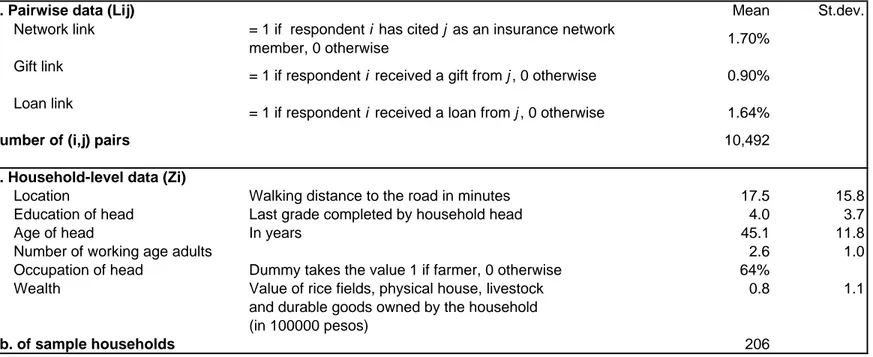
We now turn to econometric analysis. De…nitions and descriptive statistics for all the variables used in the regressions are given in Table 4. Our …rst dependent variable Lij is a dichotomous variables equal to 1 if a network link exists between households i and j. For the analysis presented here, a network link is de…ned to exist between i and j if household i cited household j as source of mutual insurance. In order to investigate the bene…ts Bij of network links, we examine ‡ows of gifts and loans between the two households. In our analysis of gifts, Bij = 1 if i receives a gift from j, 0 otherwise. The same thing is done for loans.5

Regarding regressors, we consider six types of social and geographical distance. As has been emphasized in the literature on informal risk sharing (e.g. Fafchamps 1992, Coate & Ravallion 1993, Ligon, Thomas & Worrall 2001), monitoring and enforcement mechanisms are related to the issue of the expected duration of a relation. In the context of the rural Philippines, households who reside close to each other can expect to interact for an extended period of time. Geographical proximity is thus expected to help alleviate monitoring and enforcement di¢ culties –and hence to lower the cost of establishing and maintaining a link. To the extent that incomes are spatially correlated, it also reduces the potential for income pooling. But it opens more opportunities for helping each other in case of health shocks: proximity indeed makes it easier to provide home care, to comfort the bereaved, and to assist with visits to health facilities.

In our analysis, geographical distance is measured by two variables. The …rst one is a dummy variable taking value 1 if both households i and j reside in the same ’sitio’, a small cluster of 15 to 30 households. The anthropological literature describes sitios as traditional

5

Information on gifts and loans received comes from responses given by household i. Except in a couple of cases, this information is equal to information on gifts and loans given by household j.

(15)

community groups composed mainly of kin.6 Living in the same sitio is thus related to kinship and should thus reduce monitoring and enforcement problems. The second variable captures the di¤erence between i’s and j’s distance to the nearest road, provided they reside in the same sitio. Presumably, if households in the same sitio are at the same distance from the nearest road, they are close geographically.

We focus on …ve dimensions of social distance: occupation, age, education, household size, and wealth. We expect bene…ts from the pooling of income risk to be largest between people with di¤erent occupations, and especially high between farmers and non-farm workers. Farming risk is primarily determined by weather conditions and pest infestation. Non-farm income risk, in contrast, is largely in‡uenced by demand for crafts by traders and tourists visiting the area. Consequently we expect both sources of risk to be largely uncorrelated with each other. This is con…rmed by the data which show a very low – and non-signi…cant – 0.06 correlation between farm and non-farm income.

At the same time, both farming and non-farm incomes have a large collective risk component, making us suspect that income pooling within each occupation is fairly ine¤ective at reducing risk. If households form network links to pool income risk and the cost of forming links across occupations is not too high, we expect surveyed households to form risk sharing links primarily with people from other occupations. Occupation is captured by a dummy variable that takes value 1 if a respondent is a farmer, and 0 otherwise.

As pointed out earlier, income pooling is not the only form that risk sharing can take. Taking

6

E.g., http://countrystudies.us/philippines/42.htm: “In the rural Philippines, traditional values remained the rule. The family was central to a Filipino’s identity, and many sitios were composed mainly of kin. Kin ties formed the basis for most friendships and supranuclear family relationships. Filipinos continued to feel a strong obligation to help their neighbors– whether in granting a small loan or providing jobs for neighborhood children, or expecting to be included in neighborhood work projects, such as rebuilding or reroo…ng a house and clearing new land. The recipient of the help was expected to provide tools and food. Membership in the cooperative work group sometimes continued even after a member left the neighborhood. Likewise, the recipient’s siblings joined the group even if they lived outside the sitio. In this way, familial and residential ties were intermixed.”

(16)

care of the sick and elderly is another. Di¤erences in terms of age raise the potential for risk pooling: presumably, young households with many children face quite di¤erent health risks from the elderly. Di¤erences in age are also likely to be associated with di¤erences in lifestyle, perhaps reducing social interaction across groups. Again, if bene…ts from pooling risk across categories outweigh the cost of linking up, we expect more links between di¤erent age groups.

Education is included because it is a measure of social distance but also because it is a possible source of insurance. In poor societies such as the one we study, knowledge is valuable, particularly regarding contacts with the outside world (e.g., government authorities, cooperative bank, health facilities, traders, extension agents). To rural dwellers, educated households may thus be seen as providing some protection against abuse in dealings with the outside world. Educated households may also be less vulnerable (Glewwe & Hall 1998) and recover more easily from collective shocks (Barrett, Sherlund & Adesina 2004). For this reason, we expect gains from risk sharing to be higher between households with di¤erent education levels. However, di¤erences in education level may also increase social distance and make socialization more di¢ cult (Mogues & Carter 2005).

The remaining measures of social distance are wealth and number of adults of working age in the household. Households with better education, more income earning individuals, and more wealth probably have higher incomes as well. To the extent that absolute risk aversion is decreasing with income, as is customarily assumed, households with high average income are in a good position to o¤er insurance to poorer households (Fafchamps 1999). Risk sharing may also have a redistribution component and the rich may be expected to help the poor, irrespective of risk sharing. For these two reasons, establishing links with richer and larger households is attractive to poor, small households. Rich households, in contrast, would see less need for links with poor households –or may not even see them as source of insurance. Households with more

(17)

adults of working age are also likely to need insurance less because they may pool individuals with di¤erent income pro…les and hence already achieve quite a bit of income pooling within the household (e.g. Binswanger & McIntire 1987, Fafchamps 2003).

Because insurance a¤ects income and thus the ability to accumulate assets, wealth is po-tentially endogenous to the network formation process: households with better networks may accumulate more wealth. For this reason we instrument individual wealth using variables that predate the purposive formation of insurance links, namely: education of head; value of the inheritance of the head; value of the inheritance of the spouse; whether the head was born in village of current residence; whether the household head is male; and head’s number of siblings. Instruments have a strong predictive power. Predicted household wealth from this regression is used throughout in lieu of actual wealth in the analysis presented below.

It would have been useful to include a measure of relatedness between all households in the sample. Unfortunately, this information was only collected for linked households. Consequently, we cannot formally investigate whether family is a strong link determinant. To the extent that relatives reside near each other, as seems to be the case in the study area (see above), geographical proximity may capture some relatedness e¤ects. It would also have been interesting to contrast male and female networks. Because nearly all respondents are male household heads, our data does not allow an investigation of this issue.

5.2. Network formation

We begin by estimating equation (2.4). By construction, geographical distance variables are symmetrical; as they are link attributes, they enter the regression as such. In contrast, each individual attribute is used to construct two regressors of the form zi zj and zi+ zj. Since the dependent variable Lij is directional – i may cite j as source of help even if j does not cite i –

(18)

we do not need to satisfy the requirement that regressors be symmetrical. Hence zi zj enters the regression as such, not in absolute value.

As explained in the econometrics section, we can only estimate the coe¢ cient of zi + zj regressors if individuals have di¤erent degrees. In the survey, each respondent was asked to name individuals who could assist in times of trouble. Enumerators were instructed to ask for the names of the four most important such individuals. Some respondents, however, could not give four names, and some volunteered more than four names and refused to identify the most important four. As a result the number of network partners recorded in the survey varies a little bit across respondents.7 What is important to realize, though, is that the survey did not seek to measure the degree of each respondent. We thus do not have a strong basis for identifying level e¤ects zi + zj. Although, in practice, the degree variation present in the sample makes identi…cation possible, the resulting estimates may not be reliable. For this reason, we estimate our model with and without level e¤ects.

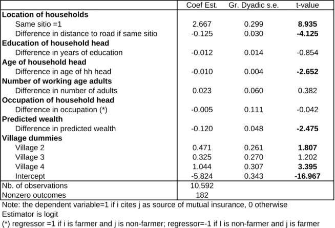
Table 5 presents our …rst set of logit estimates without level e¤ects.8 Robust dyadic standard errors are reported throughout. Village (barangay) dummies are included to control for possible village e¤ects. Geographical e¤ects appear strongly signi…cant: respondents are much more likely to cite someone residing in the same sitio as a mutual insurance link. Conditional on living in the same sitio, respondents are also more likely to cite someone close to them within the sitio. Geographical proximity is unambiguously a strong predictor of network links. As we pointed out earlier, spatial proximity reduces the scope for pooling agronomic risk (pests, ‡oods, landslides) but it facilitates monitoring and enforcement. It also makes it easier to look after a sick neighbor and thus enhances the scope for pooling health risk.

7_{Additional degree variation arises when we restrict our attention to network partners who are themselves in}

the sample.

8_{The reader may worry that logit may not be appropriate in this case given the very small proportion of}

(19)

The age di¤erence variable is signi…cant: younger heads of household are more likely to mention a link with an older household. This is consistent with the pooling of health risk, although it could also be the result of life cycle e¤ects or intergenerational altruism. Wealth is also signi…cant: consistent with expectations, households are more likely to mention as source of insurance households that are richer than themselves.

Contrary to expectations, education, occupation, and number of working age adults are not signi…cant. The big surprise is that occupation is not signi…cant: households primarily involved in farming activities are not more likely to be linked with people from other occupations. These results suggest that pooling idiosyncratic income risk is probably not the driving motivation behind network formation in rural areas. It may well be the motivation for the formation and maintenance of links with distant migrants (e.g. Lucas & Stark 1985, Rosenzweig & Stark 1989, Lauby & Stark 1988), but we cannot test this hypothesis with our data.

Model mispeci…cation may explain the lack of signi…cance of regressors. One particular cause for concern is the possible symmetry – or non-directional nature – of network links. Since the dependent variable is directional (i may cite j while j does not cite i), we have assumed that regressors enter in the form zi zj. It is conceivable, however, that the network relationship should be considered as symmetrical and hence that regressors should enter in the form jzi zjj. The zi zj formulation implies, for instance, that if the young are more likely to cite the old, the old are less likely to cite the young. It is conceivable that what matters instead is absolute age di¤erences, i.e., that the young might cite the old and the old cite the young.

To investigate this possibility, in Table 6 we reestimate the model by letting the coe¢ cient of all …ve social distance regressors di¤er depending on whether zi zj is positive or negative. If the correct speci…cation is directional –the zi zjform –then the coe¢ cients should be identical with the same sign. If, in contrast, the correct speci…cation is symmetrical – the jzi zjj form

(20)

– then the coe¢ cients should be identical and signi…cant but with opposite signs. By nesting both speci…cations, this approach enables us to investigate symmetry.

Results indicate that coe¢ cients for education, occupation, and number of working age adults remain non-signi…cant. This means that lack of signi…cance is not due to falsely assuming a directional relationship. In contrast, we …nd some weak evidence that the e¤ect of age is symmetrical. We have already seen that young household heads are more likely to cite old household heads as source of insurance. Table 6 shows that old household heads are also more likely to cite young household heads, although the e¤ect is not signi…cant. Finally, predicted wealth is no longer signi…cant, probably because of multicollinearity.

Next we check the robustness of our results in the presence of level e¤ects. As emphasized earlier, the coe¢ cients of level e¤ects may not be estimated reliably in our data, so we will not discuss their interpretation in much detail. Regression results are presented in Table 7. Our …ndings are basically unchanged for wealth di¤erences and for geographical distance variables. The age di¤erence variable is no longer signi…cant. The only signi…cant zi + zj variable is the number of working age adults in the household: links are less likely to be reported between households with many working age adults. This is consistent with the view that large households themselves serve to pool risk, thereby reducing the need for networking (e.g. Binswanger & Rosenzweig 1986, Binswanger & McIntire 1987, Fafchamps 2003).

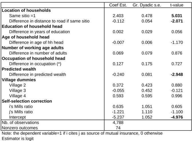
Another possible source of concern is that households may locate close to other households with whom they wish to pool income risk. This could explain why spatial proximity is strongly signi…cant while occupation and education are not. To investigate this possibility, we reestimate the model only with household heads residing in the village of their birth. We also correct for self-selection. The probit selection equation is shown in Appendix 2. The dependent variable is 1 if the household head is living in the village of birth, 0 otherwise. Two regressors are used:

(21)

birth order and whether inherited paddy land. Given the local culture (Quisumbing 1994), we expect …rst borns to remain close to their parents, and thus to live in the village of their birth. The same reasoning applies to paddy …elds since land received from parents is likely to be in the village of birth. Results con…rm that birth order is a strong predictor of residence in birth village; conditional on birth order, inherited land is not signi…cant.

Results from the selection equation are used to construct Mills ratio for each respondent i and j. These Mills ratio are then included in the dyadic regression as additional regressors. Regression results using this procedure are reported in Table 8 (without level e¤ects). Although the number of observations is much smaller, results are unchanged for geographical proximity and wealth di¤erences. This suggests that our non-signi…cant results regarding occupation, education, and number of working age adults are not the consequence of endogenous household placement.

To further investigate these …ndings, we reestimate the model with the income correlation between i and j as additional regressor. If households pool income risk, we expect a negative sign on pairwise income correlation. Endogeneity bias may arise if households engage in di¤erent activities because a link exists between them. If this is the case, income correlation would be signi…cant even though income pooling was not a motivation behind network formation. If income correlation is not signi…cantly negative, however, this constitutes additional evidence that households do not link to pool income risk. Results, not shown here to save space, yield a positive but non signi…cant coe¢ cient on income correlation, both with and without level e¤ects. Other coe¢ cients are una¤ected.

Taken together, these results suggest that, in our study area, the bene…ts from sharing income risk across occupations are not strong enough to outweigh the costs. The strength of geographical proximity e¤ects and the signi…cance of age di¤erences (without level e¤ects) and

(22)

number of working age adults (with level e¤ects) are consistent with the pooling of health risk, although they could also be explained by monitoring and enforcement considerations coupled with intergenerational altruism. Additional evidence in support of the pooling of health risk is nevertheless provided by Fafchamps & Lund (2003) who show that health risk –and especially mortality risk –is the leading motivation behind gifts and transfers: in the study area gifts and loans respond to health shocks but not to pure income shocks such as unemployment.

5.3. Bene…ts from network links

Having investigated the determinants of network formation, we now test whether links actually provide bene…ts. To this e¤ect, we estimate a model of the form:

Bij = Lij+ X

k

kdkij + uij (5.1)

where Bij is a yet-to-be-de…ned bene…t ‡owing from j to i, Lij as before is a dummy variable denoting the existence of a network link, and the dk_ij’s are the social and geographical distance variables discussed in the preceding section. Coe¢ cient in regression model (5.1) can be seen as measuring the e¤ect of a link on bene…t ‡ows, i.e., B(dij; 1) B(dij; 0) in our earlier notation. If > 0, this indicates that having a link facilitates the ‡ow of bene…t Bij.

Two types of ‡ows are examined here: gifts and loans. Fafchamps & Lund (2003) have shown that, in the study area, informal loans and gifts play an important risk sharing function. Fafchamps & Gubert (2002) have further demonstrated that loan repayment is also made con-tingent on shocks a¤ecting borrowers. This is primarily achieved by setting zero interest rate on most informal loans, forgiving interest rate in case of late payment, and letting borrowers repay in labor. It is therefore reasonable to examine whether gifts and loans indeed are more likely between households who claim to be in a risk sharing relationship.

(23)

For this test to be valid, we need to control for geographical and social distance. Indeed, even if networks played no role in actual risk sharing, distance may still a¤ect gift and loan ‡ows. Failing to control for distance would result in omitted variable bias since we already know that Lij is a¤ected by distance.

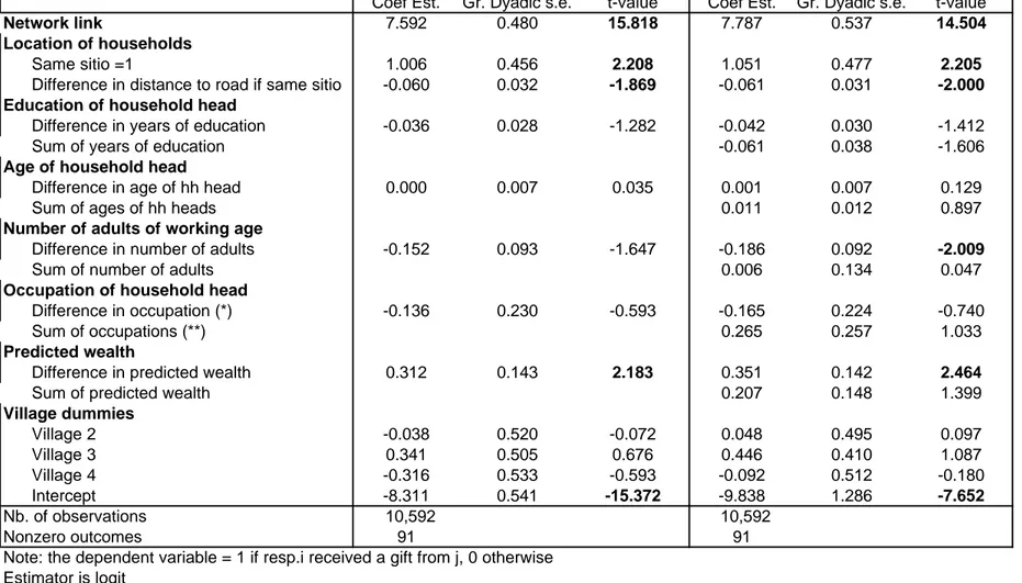
Regression results are presented in Table 9 for gifts and Table 10 for loans. In both cases the dependent variable is a dummy that takes value 1 if i received a gift (loan) from j over the three month recall period before the survey. As before, we report robust dyadic standard errors and we estimate the model with and without level e¤ects.

It is immediately clear from the results reported in Table 9 that the existence of a network link is a major determinant of gifts: the variable is strongly signi…cant, with a large t-value.9 Although many gifts take place outside networks, this result constitutes strong evidence that the existence of a network link makes a gift more likely. Geographical proximity variable are also strongly signi…cant, with the same sign as in the network formation regression. Wealthy households are more likely to receive gifts from poor households, a …nding in line with models of patronage developed by Platteau (1995a), Platteau (1995b) and Fafchamps (1999). Since wealth is instrumented using pre-determined variables, this cannot be attributed to reverse causation. These results are quite robust and remain unchanged if we limit the regressions to respondents born in their village of residence and correct for possible self-selection.

As before we check for symmetry by letting coe¢ cients di¤er for positive and negative re-gressor values. In contrast with earlier results for network formation where symmetry was not an issue, we …nd here that age di¤erences favor the exchange of gifts in both directions. Put di¤erently, the young receive more from the old and the old also receive more from the

9

The reader may worry about a possible reverse causality between gifts received and individuals listed as source of mutual insurance. To investigate this possibility we reestimated the regression without data from the …rst survey round. Very similar results obtain if we only use the second and third rounds of data collection.

(24)

young. This suggests some sort of gift exchange across generations. We also cannot re-ject the hypothesis that both coe¢ cients are the same, indicating that the likelihood of a gift between two households depends on the absolute age di¤erence between their household heads. This interpretation is consistent with anthropological evidence from the study area (e.g. Conklin 1980, Barton 1969, Russell 1987, Milgram 1999).10

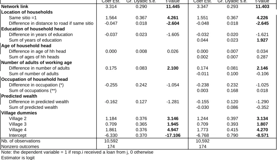
Turning to loans (Table 10), we again …nd a strong signi…cant e¤ect of a pre-existing network link. As for gifts, geographical distance has a signi…cant independent e¤ect on loans in addition to the e¤ect it has on the formation of network links. This suggests that surveyed households are more likely to obtain loans from neighbors even if they did not beforehand consider themselves connected to them. Di¤erences in wealth seem to have no e¤ect on informal borrowing, but di¤erences in household size do: larger households borrow from smaller households, strangely suggesting that households with more income earning potential borrow more. Perhaps they can do so because they have more loan repayment capacity. Finally, we …nd that more lending takes place between household with educated household heads, possibly for a similar reason. Neither of these two e¤ects survives when we limit our analysis to respondents born in their village of residence, indicating that neither result is very robust. We …nd no evidence of symmetry.

To verify the interpretation of our results, we reestimate the regressions with the income correlation between i and j as additional regressor. If households pool income risk, we expect a negative sign on pairwise income correlation: as shown by Fafchamps & Lund (2003), households that experience positive shocks are in a better position to give or lend to households experiencing a negative shock. Detailed regression results are not shown here to save space. They show that the correlation variable is never signi…cant in the gift regression, but it is strongly negatively

1 0

It also is in line with the observation made by Fafchamps & Lund (2003) that many of the gifts captured in the survey have a ’ritual’ or ’customary’ connotation – especially those made following illness or death. Many gifts recorded in the survey take a ritual form. What our analysis suggests is that these rites and customs are not anonymous rules of behavior but are embedded in interpersonal networks.

(25)

signi…cant in the loan regression –t-values of 2.8 in the loan regressions with and without level e¤ects. This suggest that loans tend to take place between households with less correlated incomes. The network link variable, however, retains all its signi…cance, indicating that pre-existing links in‡uence lending ‡ows separately from income shocks. This …nding con…rms earlier results from Fafchamps & Lund (2003) that show that network links in‡uence risk sharing through gifts and informal loans.

6. Conclusion

In this paper we have examined the formation of risk sharing networks. It is indeed increasingly recognized that informal risk sharing plays a major role in the way the rural poor deal with risk (e.g. Rosenzweig & Wolpin 1988, Townsend 1994, Ligon, Thomas & Worrall 2001) and that interpersonal networks facilitate informal risk sharing (e.g. Fafchamps 1992, Dercon & de Weerdt 2002, Fafchamps & Lund 2003, Dercon & Krishnan 2000).

In the conceptual section, we argued that social and geographic distance between households often raises the potential bene…ts from risk pooling but also the cost of establishing and main-taining interpersonal links. The net e¤ect of distance on link formation is therefore theoretically indeterminate since it depends on the net e¤ect of the di¤erence between bene…ts and costs. If costs rise su¢ ciently rapidly with distance, the pooling of risk across households with di¤erent income pro…les will not be achieved. The e¢ ciency of informal risk pooling thus depends on the way risk sharing networks are formed.

We investigated this issue empirically using a speci…cally designed survey in rural Philip-pines. We examined which dimensions of social and geographical distance predict the existence of risk sharing relationships. We found that geographic proximity is a major determinant of in-terpersonal relationships, possibly because it captures kith and kin relationships and facilitates

(26)

monitoring and enforcement, possibly because it enables households to pool health risk more easily.

Age di¤erences play an important role in the formation of risk sharing links. Fafchamps & Lund (2003) showed that gifts and loans in the study area respond to health shocks but not to pure income shocks. Taken together, their results and ours suggest that in our study area risk sharing relationships are created more with health shocks than income smoothing in mind. This stands in contradiction with much of the literature which has focused nearly exclusively on income risk.11 More research should be devoted to how informal risk sharing helps household deal with health risk.

We also …nd that households are much more likely to receive a gift or loan from someone with whom they had a pre-existing relationship, controlling for other proximity factors. Most gifts and informal loans are thus embedded in interpersonal relationships that are largely determined by social and geographical proximity.

The literature has shown that income risk is not e¢ ciently pooled in village economies (e.g. Townsend 1994, Ligon, Thomas & Worrall 2001, Foster & Rosenzweig 2001, Fafchamps & Lund 2003). This paper suggests that villagers do not appear to purposefully form links with individuals who either have a di¤erent income pro…le or who have enough wealth and human capital to assist them. In these conditions, it is hardly surprising that e¢ cient income risk sharing has consistently been rejected among the rural poor. Having found why e¢ ciency is not achieved, the challenge is now to …nd ways of encouraging risk pooling across income pro…les and wealth levels.

This paper also makes a methodological contribution to the burgeoning empirical literature on economic networks (e.g. Krishnan & Sciubba 2004, Goyal, van der Leij & Moraga-Gonzalez

(27)

2004, Fafchamps, Goyal & van der Leij 2005). First we clarify identi…cation issues in dyadic data, especially with respect to symmetry and degree distribution. Second we facilitate inference on network processes by extending the calculation of robust standard errors to dyadic data. These methodological improvements should assist other researchers working on dyadic data.

References

Bala, Venkatesh & Sanjeev Goyal. 2000. “A Non-Cooperative Model of Network Formation.” Econometrica 68(5):1181–1229.

Baltagi, Badi H. 1995. Econometric Analysis of Panel Data. Chichester: Wiley.

Bandiera, Oriana & Imran Rasul. 2002. Social Networks and Technology Adoption in Northern Mozambique. Technical report CEPR London: . Discussion Paper 3341.

Bardhan, Pranab. 1984. Land, Labor and Rural Poverty. New York: Columbia U.P.

Barr, Abigail. 2000. “Social Capital and Technical Information Flows in the Ghanaian Manu-facturing Sector.” Oxford Economic Papers 52(3):539–59.

Barrett, Christopher B., Shane M. Sherlund & Akinwumi A. Adesina. 2004. “Macroeconomic Shocks, Human Capital and Productive E¢ ciency: Evidence from West African Rice Farm-ers.” (mimeograph).

Barton, Roy F. 1969. Ifugao Law. Berkeley: University of California Press, 2nd edition.

Basu, Kaushik. 1986. “One Kind of Power.” Oxford Econ. Papers 38:259–282.

Bernstein, Lisa. 1992. “Opting Out of the Legal System: Extralegal Contractual Relations in the Diamond Industry.” Journal of Legal Studies XXI:115–157.

(28)

Bernstein, Lisa. 1996. “Merchant Law in a Merchant Court: Rethinking the Code’s Search for Immanent Business Norms.” University of Pennsylvania Law Review 144(5):1765–1821.

Binswanger, Hans P. & John McIntire. 1987. “Behavioral and Material Determinants of Produc-tion RelaProduc-tions in Land-Abundant Tropical Agriculture.”Econ. Dev. Cult. Change 36(1):73– 99.

Binswanger, Hans P. & Mark R. Rosenzweig. 1986. “Behavioral and Material Determinants of Production Relations in Agriculture.” Journal of Development Studies 22, no. 3:503–539.

Bloch, F., Garance Genicot & Debraj Ray. 2004. “Social Networks and Informal Insurance.” (mimeograph).

Coate, Stephen & Martin Ravallion. 1993. “Reciprocity Without Commitment: Characterization and Performance of Informal Insurance Arrangements.” J. Dev. Econ. 40:1–24.

Conklin, Harold. 1980. Ethnographic Atlas of Ifugao: A Study of Environment, Culture and Society in Northern Luzon. New Haven: Yale University Press.

Conley, T.G. 1999. “GMM Estimation with Cross-Sectional Dependence.” Journal of Econo-metrics 92(1):1–45.

Dercon, Stefan & Joachim de Weerdt. 2002. Risk-Sharing Networks and Insurance Against Ill-ness. Technical report CSAE Working Paper Series No. 2002-16, Department of Economics, Oxford University Oxford: .

Dercon, Stefan & Pramila Krishnan. 2000. “In Sickness and in Health: Risk-Sharing within Households in Rural Ethiopia.” Journal of Political Economy 108(4):688–727.

(29)

Fafchamps, Marcel. 1992. “Solidarity Networks in Pre-Industrial Societies: Rational Peasants with a Moral Economy.” Econ. Devel. Cult. Change 41(1):147–174.

Fafchamps, Marcel. 1999. “Risk Sharing and Quasi-Credit.”Journal of International Trade and Economic Development 8(3):257–278.

Fafchamps, Marcel. 2003. Rural Poverty, Risk and Development. Cheltenham (UK): Edward Elgar Publishing.

Fafchamps, Marcel. 2004. Market Institutions in Sub-Saharan Africa. Cambridge, Mass.: MIT Press.

Fafchamps, Marcel. 2005. “Development and Social Capital.” Journal of Development Studies . (forthcoming).

Fafchamps, Marcel & Bart Minten. 1999. “Relationships and Traders in Madagascar.” Journal of Development Studies 35(6):1–35.

Fafchamps, Marcel & Bart Minten. 2002. “Returns to Social Network Capital Among Traders.” Oxford Economic Papers 54:173–206.

Fafchamps, Marcel & Flore Gubert. 2002. “Contingent Loan Repayment in the Philippines.” (mimeograph).

Fafchamps, Marcel, Sanjeev Goyal & Marco van der Leij. 2005. “Scienti…c Networks and Coau-thorship.” (mimeograph).

Fafchamps, Marcel & Susan Lund. 2003. “Risk Sharing Networks in Rural Philippines.”Journal of Development Economics 71:261–87.

(30)

Foster, Andrew D. & Mark R. Rosenzweig. 1995. “Learning by Doing and Learning from Oth-ers: Human Capital and Technical Change in Agriculture.” Journal of Political Economy 103(6):1176–1209.

Foster, Andrew D. & Mark R. Rosenzweig. 2001. “Imperfect Commitment, Altruism and the Family: Evidence from Transfer Behavior in Low-Income Rural Areas.” Review of Eco-nomics and Statistics 83(3):389–407.

Genicot, Garance & Debraj Ray. 2003. “Group Formation in Risk-Sharing Arrangements.” Review of Economic Studies 70(1):87–113.

Glewwe, Paul & G. Hall. 1998. “Are Some Groups More Vulnerable to Macroeconomic Shocks than Others? Hypothesis Tests Based on Panel Data from Peru.” Journal of Development Economics 56(1):181–206.

Good, P. 2000. Permutation Tests: A Practical Guide to Resampling Methods for Testing Hypotheses. Springer.

Goyal, Sanjeev, Marco van der Leij & Jose Luis Moraga-Gonzalez. 2004. “Economics: An Emerging Small World?” (mimeograph).

Granovetter, M. 1985. “Economic Action and Social Structure: The Problem of Embeddedness.” Amer. J. Sociology 91(3):481–510.

Granovetter, Mark S. 1995. Getting a Job: A Study of Contacts and Carreers. Chicago: Uni-versity of Chicago Press. 2nd edition.

Hubert, L.J. & J. Schultz. 1976. “Quadratic Assignment as a General Data Analysis Strategy.” British Journal of Mathematical and Statistical Psychology 29:190–241.

(31)

Johnson, Simon, John McMillan & Christopher Woodru¤. 2002. “Courts and Relational Con-tracts.” Journal of Law, Economics, and Organization 18(1):221–77.

Krackhardt, David. 1987. “QAP Partialling as a Test of Spuriousness.” Social Networks 9:171– 86.

Kranton, Rachel & Deborah Minehart. 2001. “A Theory of Buyer-Seller Networks.” American Economic Review 91(3):485–508.

Krishnan, Pramila & Emanuela Sciubba. 2004. Endogenous Network Formation and Informal Institutions in Village Economies. Technical report Cambridge Working Paper in Economics No. 462 Cambridge: .

Lauby, J. & O. Stark. 1988. “Individual Migration as a Family Strategy: Young Women in the Philippines.” Population Studies 42:473–86.

Ligon, Ethan, Jonathan P. Thomas & Tim Worrall. 2000. “Mutual Insurance, Individual Savings, and Limited Commitment.” Review of Economic Dynamics 3(2):216–246.

Ligon, Ethan, Jonathan P. Thomas & Tim Worrall. 2001. “Informal Insurance Arrangements in Village Economies.” Review of Economic Studies 69(1):209–44.

Lucas, Robert E.B. & Oded Stark. 1985. “Motivations to Remit: Evidence from Botswana.” J. Polit. Econ. 93 (5):901–918.

Lund, Susan. 1996. “Informal Credit and Risk-Sharing Networks in the Rural Philippines.” (unpublished Ph.D. thesis).

Meillassoux, Claude. 1971. The Development of Indigenous Trade and Markets in West Africa. Oxford: Oxford University Press.

(32)

Milgram, B. Lynne. 1999. Crafts, Cultivation, and Household Economies: Women’s Work and Positions in Ifugao, Norther Philippines. In Research in Economic Anthropology. Vol. 20 Stamford, Conn.: Barry L. Isaac (ed.), JAI Press pp. 221–61.

Mitchell, J. Clyde. 1969. Social Networks in Urban Situations: Analyses of Personal Relation-ships in Central African Towns. Manchester: Manchester U. P.

Mogues, Tewodaj & Michael R. Carter. 2005. “Social Capital and the Reproduction of Inequality in Socially Polarized Economies.” Journal of Economic Inequality .

Nyblom, Jukka, Steve Borgatti, Juha Roslakka & Mikko A. Salo. 2003. “Statistical Analysis of Network Data –An Application to Di¤usion of Innovation.” Social Networks 25:175–95.

Platteau, Jean-Philippe. 1995a. “A Framework for the Analysis of Evolving Patron-Client Ties in Agrarian Economies.” World Development 23(5):767–786.

Platteau, Jean-Philippe. 1995b. “An Indian Model of Aristocratic Patronage.” Oxford Econ. Papers 47(4):636–662.

Quisumbing, Agnes R. 1994. “Intergenerational Transfers in Philippine Rice Villages: Gen-der Di¤erences in Traditional Inheritance Customs.” Journal of Development Economics 43(2):167–195.

Raub, Werner & Jeroen Weesie. 1990. “Reputation and E¢ ciency in Social Interactions: An Example of Network E¤ects.” Amer. J. Sociology 96(3):626–54.

Romani, Mattia. 2003. “Love Thy Neighbour? Evidence from Ethnic Discrimination in Informa-tion Sharing within Villages in Cote d’Ivoire.”Journal of African Economies 12(4):533–63.

(33)

Rosenzweig, Mark R. & Kenneth Wolpin. 1988. “Migration Selectivity and the E¤ect of Public Programs.” J. Public Econ. 37:470–482.

Russell, Susan. 1987. “Middlemen and Moneylending: Relations of Exchange in a Highland Philippine Economy.” Journal of Anthropological Research 43:139–61.

Shapiro, K. 1979. Livestock Production and Marketing in the Entente States of West Africa: Summary Report. University of Michigan.

Townsend, Robert M. 1994. “Risk and Insurance in Village India.”Econometrica 62(3):539–591.

Udry, Christopher. 1994. “Risk and Insurance in a Rural Credit Market: An Empirical Investi-gation in Northern Nigeria.” Rev. Econ. Stud. 61(3):495–526.

Vega-Redondo, Fernando. 2004. “Di¤usion, Search, and Play in Complex Social Networks.” (mimeograph).

(34)

Table 1- Descriptive statistics on households Sources of Income Mean (pesos) Coefficient of variation Non-farm earned income 15,178 1.77 Unearned income (1) 1,818 8.80 Value of annual rice harvest 5,596 2.49 of which crop sales 226 3.45 Net livestock sales (2) 254 11.22

Number of observations 206

(1) Includes rental income, pensions and sale of some assets (2) In terms of number of animals, fowl counts for 68%, pigs for 16%, cattle and goats for 1%, and other animals for 14%. The total average value of livestock is 2,605 Pesos and the corresponding coefficient of variation is 1.85.

(35)

Table 2. Relationship of insurance partners to household head

Close relative 488 52.0%

Distant relative 316 33.7%

Neighbor 104 11.1%

Friend 27 2.9%

Other (store owner, etc.) 4 0.4%

Total 939 100.0%

In this table, an insurance partner is a close relative when he is a son/daughter, a son/daughter in law, a grandchild, a parent or a brother/sister. He/she is a distant relative when he/she is a nephew/niece or a cousin/aunt/uncle.

(36)

Table 3. Residence of insurance partner Same barangay 596 63.5% Barangay in Banaue 151 16.1% Other Ifugao 44 4.7% Other CAR 35 3.7% Lowland 58 6.2% Manila 12 1.3% Abroad 14 1.5% Unknown 29 3.1% Total 939 100.0%

Note: The sample villages are located in the Ifugao province, within the Cordillera Administrative Region (CAR)

Banaue is the closest town, located less than 30 kilometers from the four sample villages (barangay)

(37)

Table 4- Variables used in the regressions

A. Pairwise data (Lij) Mean St.dev.

Network link = 1 if respondent i has cited j as an insurance network

member, 0 otherwise 1.70%

Gift link

= 1 if respondent i received a gift from j , 0 otherwise 0.90% Loan link

= 1 if respondent i received a loan from j , 0 otherwise 1.64%

Number of (i,j) pairs 10,492

B. Household-level data (Zi)

Location Walking distance to the road in minutes 17.5 15.8 Education of head Last grade completed by household head 4.0 3.7

Age of head In years 45.1 11.8

Number of working age adults 2.6 1.0

Occupation of head Dummy takes the value 1 if farmer, 0 otherwise 64%

Wealth Value of rice fields, physical house, livestock 0.8 1.1 and durable goods owned by the household

(in 100000 pesos)

(38)

Table 5. Network links

Coef Est. Gr. Dyadic s.e. t-value

Location of households

Same sitio =1 2.667 0.299 8.935

Difference in distance to road if same sitio -0.125 0.030 -4.125 Education of household head

Difference in years of education -0.012 0.014 -0.854

Age of household head

Difference in age of hh head -0.010 0.004 -2.652 Number of working age adults

Difference in number of adults 0.023 0.060 0.382

Occupation of household head

Difference in occupation (*) -0.005 0.111 -0.042

Predicted wealth

Difference in predicted wealth -0.120 0.048 -2.475 Village dummies Village 2 0.471 0.261 1.807 Village 3 0.325 0.270 1.202 Village 4 1.044 0.307 3.395 Intercept -5.824 0.343 -16.967 Nb. of observations 10,592 Nonzero outcomes 182

Note: the dependent variable=1 if i cites j as source of mutual insurance, 0 otherwise Estimator is logit

(*) regressor =1 if i is farmer and j is non-farmer; regressor=-1 if I is non-farmer and j is farmer regressor=0 if both are farmers or both are non-farmer

(39)

Table 6. Testing symmetry of determinants of network links

Coef Est. Gr. Dyadic s.e. t-value Location of households

Same sitio =1 2.659 0.296 8.978

Positive difference in years of education -0.018 0.034 -0.523 Negative difference in years of education -0.007 0.026 -0.283 Age of household head

Positive difference in ages of hh heads 0.010 0.009 1.058 Negative difference in ages of hh heads -0.026 0.008 -3.117 Number of working age adults

Positive difference in number of adults -0.017 0.112 -0.152 Negative difference in number of adults 0.057 0.095 0.600 Occupation of household head

i is farmer, j is non-farmer (regressor=1) 0.244 0.225 1.085 j is farmer, i is non-farmer (regressor=-1) 0.271 0.227 1.194 Predicted wealth

Positive difference in predicted wealth -0.251 0.169 -1.484 Negative difference in predicted wealth -0.036 0.118 -0.306 Village dummies Village 2 0.398 0.254 1.566 Village 3 0.259 0.254 1.020 Village 4 1.025 0.306 3.351 Intercept -6.020 0.441 -13.653 Nb. of observations 10,592 Nonzero outcomes 182

(40)

Table 7. Network links with level effects

Same sitio =1 2.402 0.476 5.043

Difference in years of education -0.002 0.028 -0.070

Sum of years of education 0.027 0.033 0.811

Difference in age of hh head -0.008 0.005 -1.460

Sum of ages of hh heads 0.014 0.010 1.454

Number of working age adults

Sum of number of adults -0.141 0.084 -1.675

Difference in occupation (*) 0.098 0.173 0.570

Sum of occupations (**) 0.057 0.222 0.255

Difference in predicted wealth -0.210 0.087 -2.424

Sum of predicted wealth 0.006 0.172 0.036

Village dummies Village 2 0.358 0.405 0.885 Village 3 -0.147 0.450 -0.326 Village 4 0.495 0.619 0.800 Intercept -6.331 1.055 -6.002 Nb. of observations 10,592 Nonzero outcomes 182

(41)

Table 8. Network links controlling for self-selection

Same sitio =1 2.403 0.478 5.031

Difference in years of education 0.002 0.029 0.056

Difference in age of hh head -0.007 0.006 -1.170

Number of working age adults

Difference in occupation (*) 0.127 0.175 0.727

Difference in predicted wealth -0.240 0.081 -2.948

Village dummies

Village 2 0.372 0.423 0.880

Village 3 -0.055 0.452 -0.121

Village 4 0.593 0.595 0.996

Self-selection correction

i's Mills ratio 0.635 1.051 0.605

j's Mills ratio -1.221 1.110 -1.100

Intercept -5.237 1.052 -4.976

Nb. of observations 4,788

Nonzero outcomes 74

(42)

Table 9. Gifts and network link

Coef Est. Gr. Dyadic s.e. t-value Coef Est. Gr. Dyadic s.e. t-value

Network link 7.592 0.480 15.818 7.787 0.537 14.504

Same sitio =1 1.006 0.456 2.208 1.051 0.477 2.205

Difference in distance to road if same sitio -0.060 0.032 -1.869 -0.061 0.031 -2.000

Education of household head

Difference in years of education -0.036 0.028 -1.282 -0.042 0.030 -1.412

Sum of years of education -0.061 0.038 -1.606

Difference in age of hh head 0.000 0.007 0.035 0.001 0.007 0.129

Number of adults of working age

Difference in number of adults -0.152 0.093 -1.647 -0.186 0.092 -2.009

Sum of number of adults 0.006 0.134 0.047

Difference in occupation (*) -0.136 0.230 -0.593 -0.165 0.224 -0.740

Difference in predicted wealth 0.312 0.143 2.183 0.351 0.142 2.464

Sum of predicted wealth 0.207 0.148 1.399

Village dummies Village 2 -0.038 0.520 -0.072 0.048 0.495 0.097 Village 3 0.341 0.505 0.676 0.446 0.410 1.087 Village 4 -0.316 0.533 -0.593 -0.092 0.512 -0.180 Intercept -8.311 0.541 -15.372 -9.838 1.286 -7.652 Nb. of observations 10,592 10,592 Nonzero outcomes 91 91

Note: the dependent variable = 1 if resp.i received a gift from j, 0 otherwise Estimator is logit

(43)

Table 10. Loans and network link

Coef Est. Gr. Dyadic s.e. t-value Coef Est. Gr. Dyadic s.e. t-value

Network link 3.314 0.290 11.445 3.347 0.293 11.403

Same sitio =1 1.564 0.367 4.261 1.551 0.367 4.226

Difference in distance to road if same sitio -0.047 0.018 -2.604 -0.048 0.018 -2.645

Education of household head

Difference in years of education -0.037 0.023 -1.605 -0.032 0.020 -1.621

Sum of years of education 0.044 0.023 1.927

Difference in age of hh head 0.000 0.008 0.026 0.000 0.007 0.034

Number of adults of working age

Difference in number of adults 0.175 0.083 2.100 0.174 0.081 2.146

Sum of number of adults -0.011 0.100 -0.106

Difference in occupation (*) -0.255 0.242 -1.054 -0.238 0.232 -1.025

Difference in predicted wealth -0.162 0.127 -1.281 -0.155 0.120 -1.290

Sum of predicted wealth -0.030 0.086 -0.352

Village dummies Village 2 1.184 0.376 3.146 1.244 0.397 3.134 Village 3 0.709 0.365 1.945 0.709 0.393 1.807 Village 4 1.861 0.376 4.947 1.773 0.415 4.270 Intercept -6.330 0.370 -17.106 -6.768 0.790 -8.571 Nb. of observations 10,592 10,592 Nonzero outcomes 174 174

Note: the dependent variable = 1 if resp.i received a loan from j, 0 otherwise Estimator is logit

(44)

Appendix 1. Wealth instrumenting equation

Coef. t

Head was born in the same barangay 0.099 1.110

Head is male 0.300 1.930

Education of head 0.035 2.040

Number of children in head's family of origin -0.010 -0.540

Value of the inheritance of the head 0.933 6.680

Value of the inheritance of the spouse 1.046 5.220

Intercept -0.243 -1.450

Nb. of observations 206