A multiscale separated representation to compute the mechanical behavior of composites with periodic microstructure
Texte intégral
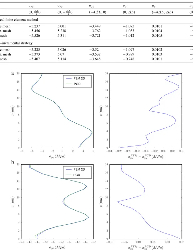
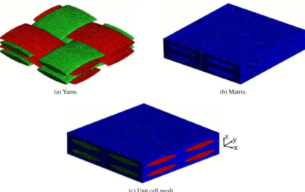
Figure


Documents relatifs
In case of soft impact, with a finite time duration of the shock, and no external excitation, the existence of periodic solutions, with an arbitrary value of the
5 compares the results obtained from the ILES computation based on Roe scheme, and the DG-VMS simulation using a low-dissipative Roe scheme with α = 0.1, for which the best
Sous des hypoth` eses usuelles sur le maillage pour des probl` emes non-lin´ eaires, sur la r´ egularit´ e des coefficients et des donn´ ees, et sur les formules de
We shall start with a short description of the three main numerical methods in shape optimization, namely the boundary variation, the homogenization and the level set methods.. For
However, for the situations considered, even when iterative peeling was used, ESIP with 50 000 samples yielded more accurate results in a fraction of the computing time than
We present hereafter the formulation of a Timoshenko finite element straight beam with internal degrees of freedom, suitable for non linear material problems in geomechanics (e.g.
The shapes obtained following the combination of the genetic algorithm reported in [20] and the topological optimization by the mixed relaxation/level set method are presented
iii) three boundary points do not have the same image; two boundary points having the same image cross normally,.. iv) three different points belonging to the union the
