Science Arts & Métiers (SAM)
is an open access repository that collects the work of Arts et Métiers Institute of
Technology researchers and makes it freely available over the web where possible.
This is an author-deposited version published in: https://sam.ensam.eu Handle ID: .http://hdl.handle.net/10985/8692
To cite this version :
Benoit AUGIER, Patrick BOT, Frédéric HAUVILLE, Mathieu DURAND - Experimental validation of unsteady models for fluid structure interaction: Application to yacht sails and rigs - Journal of Wind Engineering & Industrial Aerodynamics - Vol. 101, p.53-66 - 2012
Any correspondence concerning this service should be sent to the repository Administrator : [email protected]
Experimental Validation of Unsteady Models for Fluid Structure Interaction:
Application to Yacht Sails and Rigs
Benoit Augier1, Patrick Bot1, Frederic Hauville1, Mathieu Durand2
1ECOLE NAVALE - IRENAV CC600, 29240 BREST Cedex 9, France
2K-Epsilon Company, 1300 route des cretes - B.P 255 06905 Sophia Antipolis Cedex, France
Abstract
This work presents a full scale experimental study on the aero-elastic wind/sails/rig interaction in real navigation conditions with the aim to give an experimental validation of unsteady Fluid Structure Interaction (FSI) models ap-plied to yacht sails. An inboard instrumentation system has been developed on a J80 yacht to simultaneously and dynamically measure the navigation parameters, yacht’s motion, and sails flying shape and loads in the standing and running rigging. The first results recorded while sailing upwind in head waves are shown. Variations of the measured parameters are characterized and related to the yacht motion (trim mainly). Correlations between the different pa-rameters are examined. In the system’s response to the dynamic forcing (pitching motion) we attempt to distinguish between the aerodynamic effect of varying apparent wind induced by the motion and the structural effect of varying stresses and strains due to the motion and inertia. The dynamic full scale measurements presented underline the neces-sity of considering the unsteadiness of phenomena to correctly simulate a yacht’s behavior in actual sailing conditions. The simulation results from the FSI model compare very well with the experimental data for steady sailing conditions. For the unsteady conditions obtained in head waves, the first results show a good agreement between measurements and simulation.
Keywords:
Fluid Structure Interaction, Full Scale Experiment, Unsteady, Yacht Sails
1. Introduction
In the last decades, massive improvements have been made in yacht design, materials and building, as shown by the continuously increasing performances achieved by racing yachts all over the world. As yacht racing competitiveness is growing, there is an increasing need for more and more detailed research and development in the field of sailing yachts. This effort has led to many research activities both experimental and computational to better understand the behavior of racing yachts and to optimize their design and use. For example a special issue of the Journal of Wind Engineering & Industrial Aerodynamics has been devoted to sails aerodynamics (Flay (1996)). Computational Fluid Dynamics (CFD), analytical studies, tank testing and wind tunnel studies have been largely used to optimize hull, rig and sails
Email address: [email protected] (Benoit Augier1)
design (Caponnetto et al. (1999), I.M.C. (1998), Hansen et al. (2006), Schneider et al. (2003), Miyata et al. (1997)). Concerning sails aerodynamics, many studies have been made using CFD (Miyata and Lee (1999), Thrasher et al. (2001)) and model scale experiments in wind tunnels (Fossati et al. (2008, 2006), Le Pelley and Modral (2008), Fujiwara et al. (2005)) but fewer studies have been devoted to full scale trials in real navigation conditions (Clauss and Heisen (2006), Masuyama et al. (2009), Viola and Flay (2010a,b)). Recently, several authors have focused their interest on the Fluid Structure Interaction (FSI) problem to address the issue of the impact of the structural deformation on the flow and hence the aerodynamic forces generated (Chapin and Heppel (2010), Renzsh and Graf (2010)). The FSI problem of yacht sails is complex because the structural and aerodynamic problems are highly and non-linearly coupled, and as the sails are soft structures, even small stresses may cause large displacements and shape changes leading to high variations in the aerodynamic
forces. Moreover, this aero-elastic problem is unsteady because of wind variations and more importantly yacht motion due to the sea state and crew actions. Very few studies have addressed the unsteadiness issue of sails aerodynamics. A first attempt to consider unsteady conditions for the flow on yacht sails was made by Charvet et al. (1996). Gerhardt et al. (2008) investigated the unsteady aerodynamic phenomena associated with sailing upwind in waves on a simplified 2D geometry. Fossati and Muggiasca (2009, 2010, 2011) studied the aerodynamics at model scale in a wind tunnel, and Viola and Flay (2010a,b) achieved full scale pressure measurements on sails. To the authors’ knowledge, the present work is the first report of full scale experimental unsteady FSI study with unsteady numerical and experimental comparison. Some preliminary results of this work have been presented in Augier et al. (2010, 2011). Indeed, Fossati and Muggiasca (2009, 2010, 2011) showed that a yachts’ pitching motion has a strong and non trivial effect on aerodynamic forces. They evidenced that the relationship between instanta-neous forces and apparent wind deviates -phase shifts, hysteresis- from the equivalent relationship obtained in a steady state, which one could have thought to apply in a quasi-static approach. Very recently, in a different field of application, Michalski et al. (2011) achieved a detailed study of membrane structures under fluctuating wind loads.
In this paper, the results obtained while sailing in head waves are presented and the variations of each measured parameter are analyzed and compared to the yacht’s motion which is the dynamic forcing applied to the aero elastic system. In section 2, the FSI model used for validation is rapidly presented and the methodology developed for the experimental/numerical validation is explained. The experimental system is described in sec-tion 3. Then, the core of the paper is made of a pre-sentation and analysis with respect to yacht motion of the unsteady recorded results: apparent wind, loads and sails flying shape parameters. In the last section, simu-lation results are compared to the experimental data. 2. Fluid Structure Interaction modeling:
ARA-VANTI
The company K-EPSILON is developing a model with a strong coupling in inviscid fluid between ARA and AVANTI, root of the ARAVANTI model. Experimental validation of the ARAVANTI model is integrated in the project Voil’ENav, developed in the IRENav laboratory.
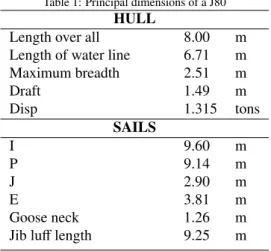
Table 1: Principal dimensions of a J80 HULL
Length over all 8.00 m
Length of water line 6.71 m
Maximum breadth 2.51 m Draft 1.49 m Disp 1.315 tons SAILS I 9.60 m P 9.14 m J 2.90 m E 3.81 m Goose neck 1.26 m Jib luff length 9.25 m
ARAVANTI is a fluid-structure model using a Constant Strain Triangles (CST) membrane elements model extended in 3 dimensions (Roux et al. (2008)). Hypoth-esis imposed inside this element are constant stresses, constant strains and uniform stiffness of the mate-rial. Non-linearities coming from the geometry and compressions are taken into account. The calculation of the flow around the sails is carried out under the hypothesis of an incompressible inviscid fluid, using a particle method developed by Rebhach (1978) and then Huberson (1986). This method is, in essence, unsteady, taking into account the slip condition on the surface as a boundary condition. A Kutta-Joukoswski condition is imposed on the trailing edge of the sail, initiating the wake of the flow. An atmospheric wind gradient is taken into account with a logarithmic law. The effects of the interaction are translated into a coupling of the kinematic equation (continuity of the normal component of the velocity at the interface between fluid and structure geometrical domains) and dynamic equations (continuity of the normal component of the external force, pressure forces, on the contact surface of the sail with the fluid).
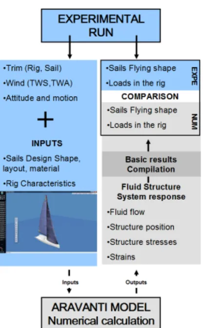
Figure 1 presents the experimental and numerical val-idation loop for the instrumented boat set up. ARA-VANTI settings are given by the trim, the wind vector and the yachts’ attitude recordings. Rig and sail geom-etry and mechanical characteristics are added as inputs. Calculation results are compared to the loads and flying shapes measured while sailing.
Figure 1: Methodology of the Numerical/Experimental data compari-son.
3. System Apparatus 3.1. Sensors arrangement
Full-scale measurements are performed on a J80 yacht, an 8.00m one-design cruiser racer boat. Principal dimensions of the J80 are presented in Table 1. A ded-icated instrumentation has been developed in order to measure the unsteady navigation loads, motion, flying shape and navigation parameters. Figure 2 shows the general arrangement of the instrumented boat with the position of sensors.
Figure 3 shows the sails geometry used in the code for the calculation. The figure also gives the name of each item of the running and standing rigging where tension is measured with the load sensors shown on figure 2.
Loads measurement is performed by instrumented fittings with stress gauges. Seven instrumented turn-buckles measure the loads on the six lateral shrouds and the Forestay and eight instrumented shackles are distributed around the different tension points of the mainsail (Outhaul, Sheet, Halyard, Cunningham and Boom Vang) and the jib (Sheet, Halyard and Tack). A ninth shackle is placed on the backstay. The 16 load sensors are connected to two dedicated analog data acquisition and synchronization Spider8 devices from HBM inside the boat.
Figure 2: Plan of a J80 with sensors general arrangement. Solid circles represent the load sensors on items defined on figure 3
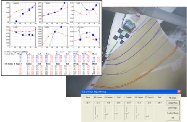
Four analog cameras are fixed on the mast, two on the mast head recording the mainsail, and two under the Forestay hound point, recording the jib. For measuring convenience, horizontal stripes are drawn on the main-sail and jib at heights of 20%, 40% and 70% of luff length. Sail shape parameters are extracted stripe by stripe from pictures by image processing software ASA and ISIS, as shown in Figure 4. Sail shape parameters are defined in Figure 6. Calibration grids are placed on the deck to determine the cameras position and angle and then tune them while post processing (Zhang (2000)). Additional cameras are fixed on the roof recording the crew and the sail foot.
Sails recorded in experiment are designed by the sail maker Delta Voiles and used in the J80 class Interna-tional championship. The mainsail is half-batten with
Figure 3: Sail Geometry from DeltaVoile with definition of each item where tension is measured with load sensors shown on figure 2
the highest section in full-batten. The jib gets a half batten on top. The sail CAD software SailPack from BSG Development is used to design the sails (design shape, cloth, panel type and orientation). ARAVANTI is coupled to SailPack in order to build the sail structure meshing from the CAD software. Sails dimensions are presented in Table 1, where I, J, P, and E are the measurement lengths of sail dimensions according to IMS rules IMS Congress (2010) (see figure 2).
Figure 4: Example of a stripe parameter image processing on a Jib with ASA sofware
The Motion sensor Xsens MTi-G is placed on the
rotation center of the hull for small angles at 0◦ heel angle. An ultrasonic 3D anemometer is fixed on the mast head and a loch has been installed on the J80’s hull. Wire displacement sensors are fixed between the main car and the boom and the jib car and the clew to measure the sheet length. The main car always remains centered during the experiments and the jib’s car position is recorded. A rudder angle sensor is fixed on the helm. A flux gate compass and a GPS are used inside the boat.
Sensors are linked to an inboard computer. Acquisition is controlled by RTmaps , a dedicated piece ofR
software for synchronization and dating developed by Intempora.
3.2. Load sensor
The use of existing calibrated load sensors, like classical S shape load sensors, was set aside because their oversize and their weight needed to modify the rigging and limited the available measurement points. Turnbuckles and shackles were instrumented with strain gauges and substituted to the basic fittings. Figure 5 shows the final stage of development of the instrumented fittings.
The dedicated load sensors were calibrated in order to estimate the error precision of each sensor. They are designed to respect the sails’ and rigging’s adjustments in normal conditions and to reflect the reality of load in the rigging’s tension points in order to get the finest measurement.
Figure 5: Instrumented shackle and turnbuckle. Strain gauges are under the black water tight mastic
Instrumented turnbuckles are the same as those used in navigation: Sparcraft turnbuckle 116mm for 5 and
4mm cable. The same adjustment for the initial load in the rigging can be done. A full bridge load gauge is stuck on two flat lugs symmetrically machine-cut on the turnbuckle shank linked to the chain plate. Turnbuckles, because of their thin shape, work in a pure traction effort. The maximum design load is 10000N. Calibration with a standard measurement load sensor from HBM presents good repeatability and the sensitivity and precision error have been determined for each sensor. The total precision error is lower than 60N for all instrumented turnbuckles.
More R&D was needed to obtain reliable sensors with the instrumented shackles. Indeed, the first cali-bration tests showed that the shackles do not work in pure traction and the measurement is affected by com-pression or bending, resulting in a poor repeatability of the measurements. The shackle sensors have then been upgraded in the following way. A diabolo has been fitted to the pin in order to keep the tension on the symmetry axis and both branches of the shackle have been equipped by a connected full-gauge bridge to av-erage the load in each side. The asymmetry of the pin, threaded on one side and linked by a pivot on the other, was shown to be a source of non-repeatability. The shackle was then machine-cut to have two bores and the pin was replaced by a bolt with nut, screwed through the branches. Calibration of the last upgraded shackles has given really good results and the absolute error for all instrumented shacles proved to be inferior to 50N. The obtained instrumented shackles and turnbuckles are shown on Figure 5
3.3. Sails flying shape
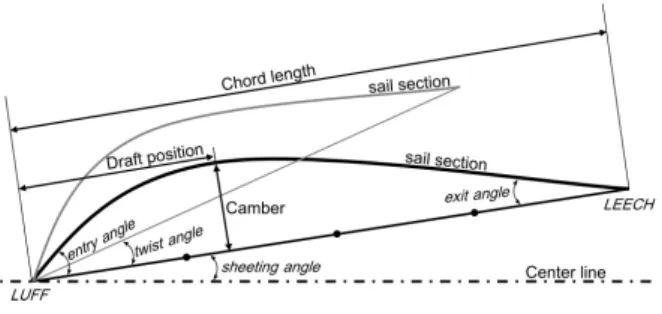
The sails flying shape is charcterized by the param-eters classically used in sail shape analysis as defined on Fig. 6 which are measured on the visualisation stripes taped on the sails at 20%, 40% and 70% of the luff length. Two sail analyzer softwares have been used to determine the flying shape parameters from the pictures: ASA and ISIS. 2D images recorded by the cameras are transformed in 3D-data in the world coordinate system to measure the sails flying shape with the hypothesis that the visualisation stripes on the sails belong to a plane parallel to a reference plane, at a known height. The position and axis of the cameras with respect to the reference plane are determined through the use of calibrated test patterns placed on the deck (see Fig. 19). To correct the lens distortion, cameras are previously calibrated using a method based on the work of Zhang (2000), inspired from the camera calibration toolbox for Matlab. Images
are corrected in post processing with the distortion coefficient determined for each camera.
To assess the calibration procedure and the sails parameters extraction, tests have been achieved on a known sail-like shape drawn on a cylindrical wall, for different camera positions and using the same test patterns. The calculated camera position differs from the actual position by less than 10mm for a distance from camera to test pattern of 4m. Concerning the sails parameters, the precision is good in general (less than a few percent) but becomes suspicious for very flat profiles particularly on the entry and exit angles: for example 3 degrees of error on a 7 degrees entry angle for a camber 1.5% of chord length. The errors mainly come from the determination of the stripe line on the image.
Figure 6: Definition of the flying shape parameters on the bottom stripe (bold line). An upper stripe is drawn to illustrate the twist angle.
Other sensors of the instrumented sailing boat, as the classical navigation equipment found in all cruisers or the wire displacement sensors, have been characterized in order to evaluate the accuracy and quantify the preci-sion errors on the measurement.
3.4. Recording unsteady data
The data acquisition application has been developed with the RTmaps software which is well adapted for real time acquisition. Sensors are free to communicate with the computer at their own frequency and each sample is stored in the buffer with its own sampling time. A resampling is applied before analysis when synchronous data are needed. The low frequency experimental data, from NMEA frame, used as inputs to the computations, as well as the loch speed, the GPS speed or the fluxgate compass heading, have been smoothed to avoid jumps which would input irrelevant noise in the simulation.
4. Results
In this paper, different runs of the yacht sailing on a close hauled course, on a single tack, are presented. The first one is a 3 minute starboard tack run in 0.80m head swell in an average wind of 12 knots (section 4.1). This run underlines the range of loads encountered at sea. The second run is a 20 second port tack run in 0.3m short head swell with a detailed unsteady analysis (sec-tion 4.2). The last one is a 10 second port tack run in rather flat sea and stable wind, where the variations of all parameters are as small as possible. This run is used for the validation of the model in steady state (section 5) with the 10 second averaged values for the input param-eters. During those runs, the yacht is driven at constant AWA, in the usual way while beating the best VMG and there is no action of the crew else than steering. 4.1. First run: Loads amplitude and range of efforts.
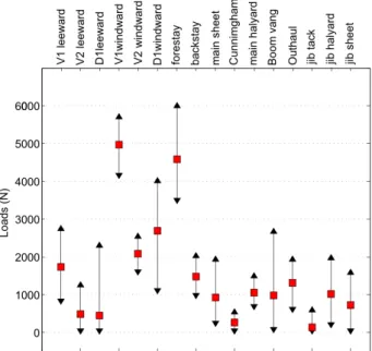
Yacht attitudes, loads in the rig and sail flying shape are unsteady by essence. The importance of the un-steadiness of sail boat navigation is well known by sailors because the optimum rig and sails adjustments in calm sea and steady wind are not the same as in waves and shifty wind. Dynamic measurement of loads in the rigging gives interesting information about the real range of tension. Figure 7 shows the mean value and loads variations encountered during this first run where the yacht is sailing in a head swell of approximate height 0.8m. This figure illustrates the high range of load vari-ations experienced by the rigging even in a moderate sea state. D1Windward, Forestay and Boom Vang are sub-ject to the highest range of variation up to 3000N, when sails tension points suffer a relative variation of more than 80%.
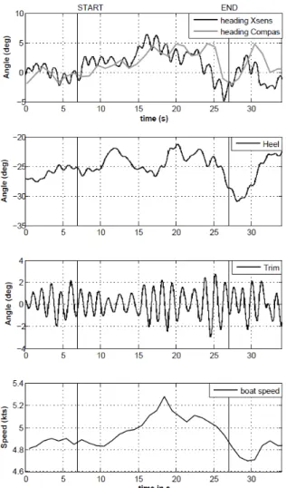
4.2. Second run: Detailed unsteady measurements This section is focused on the recordings made on a 35 second run of pitching in head swell with 20 sec-onds of special interest for comparison. The swell is short with an average period of 1.3s and 0.3m wave height. The variation of trim, heel, heading angle and boat speed is presented in Figure 8. Headings are recorded by the Xsens motion sensor and the compass. Boat speed is recorded by the loch. The bounds of the 20 seconds of interest correspond to the vertical lines marked START and END. The boat is sailing on port tack. There is no information on the jib tack because the shackle wire was broken at the beginning of the exper-imental set. The sea state and the swell are not directly measured and only the yacht motion is recorded. As the hydrodynamic yacht behavior and seakeeping are out of
Figure 7: Range of loads in the rig for a 3 minute run in 0.80m head swell. Mean Values are represented by a solid square
the scope of this work, pitching is considered as the dy-namic forcing of the rig and sails aeroelastic system.
According to the reference frame adopted for the boat and presented in Figure 2, positive values of the trim correspond to the bow diving.
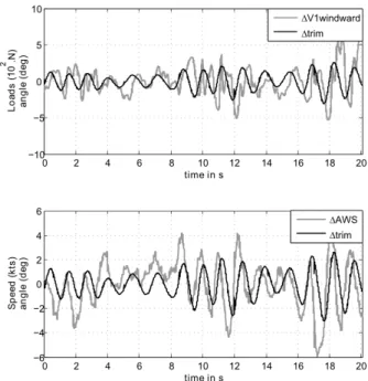
Figures 9 and 10 present the effect of pitching on sail loads, trim angle, and apparent wind angle and speed. We can notice that variations are related to the trim variation, particularly for the loads: weak variation in t ∈ [10s; 14s], strong in t ∈ [16s; 20s] and peaks at t= 25s.
Loads in the shrouds appear to be sensitive to trim angle and the pitching oscillations are contained in the loads variations. Amplitude of variation seems to be related to the load level. In fact, the windward shrouds are more sensitive to boat oscillation than those on lee side. The same conclusion can be made on the proportionality of efforts with Forestay and Backstay. D1winward has the biggest variation amplitude. The D1 shrouds contribute to the mast rake and have an important longitudinal component of efforts. The forward mast swing due to head swell will be directly transmitted to the D1windward load, added to the wind variation.
Loads in sails are also sensitive to pitching with an important relative variation due to oscillation. Mainsail outhaul and Cunningham are not represented here for legibility reasons but have the same sensitivity to
oscil-Figure 8: 35s time history of heading angle, heel angle, trim angle and boat speed in head swell.
lation. Oscillations of apparent wind angle and speed seem to be linked to pitch. In the usual definition of the apparent wind AW, the yacht motion is averaged out and the slowly varying apparent wind AW is simply defined as:
−−→
AW=−−→T W −→−V
where TW is the true wind and V is the boat speed. When considering the dynamic behavior as in the present case, we have to account for the yacht motion induced variations, such that the instantaneous apparent wind is defined as:
−−→
AWinstantaneous(OM)=
−−→
T W −→−V +→−Ω(t)Λ−−→OM+ noises Where→−Ω is the rotation velocity and−−→OMthe distance from the center of rotation to the point where AW is
Figure 9: 35s time history of loads in the rig and trim angle.
considered. Here→−Ω is mainly pitch,−−→OM=→−h distance to the top mast where AWA, AWS are measured. For instance, when the bow is diving the instantaneous AWS increases and the AWA decreases.
As shown on figures 8, 9 and 10, the pitching oscilla-tion appears in the different parameters time series. Fig-ure 11 shows the Power Spectral Density (PSD) of trim, V1portside and AWS signals. The PSD is the Fourier transform of the autocorrelation function, Cuu(τ), of the
signal u(t). PS D( f )= Z +∞ −∞ Cuu(τ)e −2πi f τ dτ where Cuu(τ)= Z +∞ −∞ u(t).u(t − τ)dt
Graphs are represented in a semi logarithmic scale. The PSD of trim shows that the trim oscillation has 2 very close frequencies: 0.69Hz and 0.85Hz. Those 2 frequencies can be explained by the 2 different swell
Figure 10: 35s time history of loads in mainsail and jib, apparent wind angle and speed, trim angle.
periods encountered during the 20s run. The PSD of AWS and V1portside contains those frequency peaks. This representation confirms that the pitch oscillation is related to loads and apparent wind. Similar peaks can be found in the PSD of all load signals and AWA.
Loads and attitude variations, as trimming, have a great influence on the flying shape. A part of the onboard instrumentation is designed to measure the variations of the sails’ shape. Observations with cam-eras from the top mast confirm the unsteady behavior of the stripes parameters. The next paragraphs are focused on the influence of a 0.30m head swell on the sails’ flying shape in a portside close hauled run.
The frame rate of video grabbers is different from one camera to another. Jib pictures are recorded around 6.5 Hz and mainsail pictures are recorded around 3.4Hz.
Figure 11: Power Spectral Density of the Forestay, trim and AWS signals. Vertical lines indicate the swell frequencies
Sails parameters have been extracted from the picture of sails, taken from the top mast. Sail analysis produces a great amount of results. Only 4s of the Jib parameters will be presented. The 70% stripe, being the highest, is the closest to the camera and achieves the best resolution.
To isolate the unsteady behavior, the mean value is subtracted from the data time series and we define:
∆u(t) = u(t) − ¯u where ¯u = 1
T
RT
0 u(t)dt with u(t) the measured signal
depending on time.
Figure 12 presents the variation, around the mean value, of the principal sail parameters, defined in Figure 6, at the 70% stripe. Parameters are linked to another measured signal in order to present their influence. Jib halyard and sheet load variations appear to affect the sum of entry and exit angle, θ. A bigger θ increases the camber and makes the draft move forward, closer to the luff. At sea, trimmers commonly adjust the halyard tension to change the sail profile. An increase of loads causes a decrease of the thickness of the sail profile and moves the draft forward.
Variations of loads in the Forestay are put in relation with the twist. An increase in Forestay load decreases the sag. The consequences are to decrease the camber and to increase the twist. The pitching oscillations in loads are present in the twist temporal evolution. Twist signal has the same period than the Forestay, subject to the pitch because of the mast trim oscillation. The increasing load in the Forestay opens the top of the sail, meaning it increases the twist angle. It highlights the influence of attitude on sail trimming and flying shape.
Figure 12: Variations of 70% Jib parameters regarding loads in rig during pitching
The sails’ flying shape depends on the design shape first, but also the trimming, the wind and the loads in tension points. The latter three parameters have a great influence and vary in time as illustrated by Figure 7-12 meaning that they have to be modeled as unsteady during the design process.
4.3. Analysis and discussion 4.3.1. Cross-correlations
Two temporal signals are said to be correlated if they have a constant relative phase. The cross-correlation quantifies how correlated the signals are. It may be interpreted in terms of cause-effect relationship. The cross-correlation quantifies the ability to predict the value of the second wave signal by knowing the value of the first one.
With Cxx(t) the auto correlation of the time series x(t)
and Cxy(t) the cross correlation of signals x(t) and y(t),
the normalized cross-correlation function Gxy(t) of time
series x(t) and y(t) is defined as: Gxy(t)=
Cxy(t)
pCxx(0).Cyy(0)
The normalized cross-correlation functions of mea-sured data have been calculated. Correlation is high between the shroud signals (≤0.85), especially the V1portside and starboard. Backstay and Forestay are also well correlated. Forestay and Backstay loads are well correlated to pitch and yaw. Main sheet is correlated to Outhaul. The plot of the normalized cross-correlation function in the time domain, as in Figure 13 in the case of trim and Backstay, gives information about the nature of correlation as in-phase or phase opposition (sign of the maximum) and the phase shift (abscissa of the maximum). The maximum is highlighted by a black square in the graph. The signals have a positive cross-correlation of 0.85 which indicates good correlation. The maximum appears for t=0.23s, which indicates a 0.23s phase lag of Backstay load oscillation.
Figure 13: Normalized cross-correlation function between the trim and the Backstay measured signals. The maximum value is 0.85 with a phase shift of 0.23s.
4.3.2. Wind group/ structure group data
As shown in the previous paragraph, loads and wind are pitch-sensitive. For loads, the amplitude of variation depends on the initial value and direction of effort (lon-gitudinal component of effort is more sensitive to struc-ture oscillation). Considering the aeroelastic response of the system to the unsteady forcing due to the sea state, two types of behavior can be distinguished. The effects of this behavior can be sorted in two groups:
• The structural group: boat motion and inertia are dominant in the behavior.
• The wind group: varying AWA and AWS, induced by boat motion, is dominant. The behavior is linked to the aeroelastic behavior.
The structural group is directly sensitive to the trim oscillation. The wind group is sensitive to the wind oscillation. Pitching period can be found in signals because the apparent wind is linked to oscillation. The Wind group signals have much more oscillation because the wind plays the role of a system response to trim.
Wind group has higher variation in amplitude by 15-25% because the influence of trim is modified by the AWA and AWS variation. The wind system response increases the effect of pitching. Structural group variation amplitudes are lower than 10%.
The trim angle is a way to observe the pitching effects on the navigation parameters and the dynamic effects on loads in the rigging. The frequency of the pitch oscilla-tion can be found in the temporal representaoscilla-tion of the load in the shrouds as presented in figure 9. The phase shift is explained because AWS is directly linked to the rotation around the y axis. AWS peaks correspond to trim(t) maximum slope. As the apparent wind is mea-sured on the mast head and the motion is recorded on the center of heel and trim rotation of the hull a phase shift may also be caused by deformation of the mast. The dynamic response of the boat is short amplitude pitching sensitive. The maximum variation due to trim oscillation presented in figure 14 gives an overspeed of 34% for the AWS and an overload of 12.5% for the V1portside. Temporal representation, with the light of a frequency and cross-correlation study, is a reliable tool to have a global idea of the load variation in the rig.
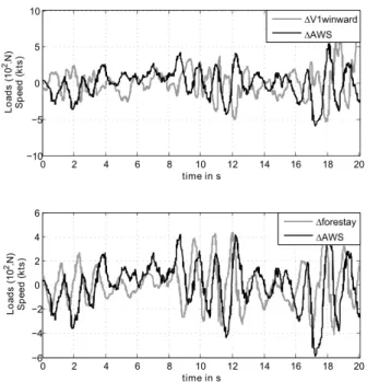
The AWS depends on the trim as illustrated in the previous paragraph. The variation of AWS due to pitching has an influence on the sails’ performance. Figure 15 shows the temporal evolution of loads in the shroud V1windward and the Forestay, while Figure 16 shows loads in Mainsail and Jib Sheets superposed to the AWS. All these parameters are in the Wind group. Oscillations and load peaks fit AWS signal in the case of sheets. The tension in sail seems to respond immediately to the apparent wind puff in the last 10 seconds of the run. Wind speed decreases have less influence on the load. Main Sheet load is totally cou-pled to AWS and suffers overloads up to 25% when the overload of Jib Sheet is 24%. Shrouds loads seem less
Figure 14: Variation of∆load in V1portside and ∆speed of apparent wind regarding to the trim.
connected to the variation of AWS according to Figure 14 and 15. The principal wind peaks are followed by an increasing load in Forestay but the general signal appearance is quite different. Pitching periods can be identified in the last 12 seconds for the Forestay. Maximum peaks represent 7.5% of the average load.
Influence of the unsteady effects and consequences on loads in shrouds and sails tension points are obvious in this temporal representation. These phenomena underline the importance of an unsteady model to simulate the flow and the stresses in sails.
4.3.3. Hysteresis
Pitching has an influence on the variation of the load in the rig as previously shown. The study of the influence of trim on loads gives information not only about the dynamic behavior and peak loads but also about the hysteresis phenomenon.
Figure 17 presents the variations of the Forestay, main sheet and Backstay load as a function of trim angle. The two loops represented correspond to two different complete periods of oscillation. Forestay and Backstay loads variations are elliptical. Reading direction is indicated by an arrow.
The hysteresis loop denotes the presence of a phase shift between loads and the pitch. If loads were perfectly
Figure 15: Temporal evolution of the∆loads in shrouds compared to the∆AWS variations.
in phase with the trim angle variation, the hysteresis loop would appear as a simple line. According to Fossati and Muggiasca (2010, 2011), a simple line is the representation of the steady state trend. Depending on the sign of the phase shift, the area inside the loop represents the amount of energy that is dissipated by the head swell pitching or added to the rig and sails. The difference between unsteady model and quasi steady model exposed by Fossati and Muggiasca (2010, 2011) is confirmed by the measurements.
The negative slope of the Forestay loop indicates that the Forestay and trim signal are in anti phase. Because Forestay load variations is delayed compared to trim, the area in the loop represents the energy due to the head swell in the rig. The Backstay hysteresis loop is nearly horizontal (zero slope) indicating that Backstay and trim have a π/2 phase shift.
Main sheet hysteresis variations are concentrated between 0 and+2 degrees of trim, as if the sheet was pulling the sail back during positive pitching. The tendency is a positive slope, meaning that Main Sheet is in phase with a late phase shift with trim signals.
Figure 16: Temporal evolution of the∆loads in sails sheets compared to the∆AWS variations.
5. Numerical and experimental comparison 5.1. Steady state
In the aim of validating the FSI model ARAVANTI, comparisons are first made on a steady state case. A 10 second run is selected because of the few variations on the static loads and navigation parameters. The boat is sailing on port tack, on a close hauled course. Experimental data of the different parameters defined as inputs (Figure 1), are given to the model: average value on 10 seconds of the trim, the rig and the sails, TWA and TWS, boat attitude. Only attitude, heel, trim and heading are imposed to the model. Motion, roll, pitch and yaw are not inputs, they are calculated from derivative of attitude. Identical sails design shape, layout, material and rig mechanical characteristics are used as model inputs for all the subsequent calculations. Figure 18 presents the numerical and experimental comparison on the loads of the instrumented sail boat based on the mean values calculated from the steady state. In this comparison, loads in sails tension points are very well evaluated. Simulation predictions fit the measured value in the case of Jib Sheet and Halyard, Main Halyard and Sheet, Outhaul, and Boom Vang. The Cunningham is working in the low part of sensor range, which may explain the discrepancy between
Figure 17: Loads variation during pitching periods
measurement and prediction.
Loads in the shrouds are also well predicted, es-pecially for the Backstay and the windward shrouds. Prediction is given with a relative error ≤8% for the windward shrouds. Leeward shroud loads, nearly slack, are quite difficult to compare because of their very low values. Forestay simulation fits experimental data within 10% relative error. Thus, we can consider that the model achieves its goal by respecting the experimental trends and by giving good estimates.
The ARAVANTI model gives a graphical repre-sentation of the calculation in order to appreciate the
Figure 18: Experimental and numerical comparison on loads for a steady state run of 10s.
simulation on the flying shape. The calculated flying shape demands for a small manual iteration loop based on the sheets’ length. Information on the sheets’ length are not precise enough in the present experimental settings. The operator needs to test different sheets lengths in order to make the calculated position of the sails clew fit the measured one.
Figure 19 shows the superposition of the calculated flying shape for the steady state and the recorded sails shot during the 10 second run.The matching is perfect for the spars, the shrouds and the main flying shape. Small discrepancies appear in the flying shape of the jib, which may be attributed to light differences in the jib structure between the sail design and the actual jib built. Actually, the number of kevlar yarns in the frames of the jib is not accurately known. Despite these small discrepancies, the calculated sails shape matches the recorded one very well, outlines and stripes fitting nicely between each other. The camber is well predicted and the draft position is placed correctly. The twist is also well predicted.
5.2. Unsteady state
The second run, pitching in head swell on port tack, has been chosen for an unsteady calculation. A steady state calculation made on 5 seconds, with parameters recorded just before the pitching, has been made in order to launch the simulation with the right loads and
Figure 19: Comparison of the experimental flying shape and the numerical result on a port tack close hauled steady state. The picture and gray visualisation stripes show the measured flying shape; the black thick lines show the computed position of the beams in the model (mast, boom, spreaders, battens); the white lines show the computed sails outline and visualisation stripes
attitude. During simulation, the boat is navigating on a constant wind of 14 knots, with a heading to North (0o)
and a TWA of 40o. Recorded variations of AWA and
AWS are assumed to come only from the boat’s motion. Recorded attitudes, from the Xsens motion sensor, are implemented as inputs. Signals are sampled at 200Hz and then smoothed in order to get a continuous second order derivative. Calculation is made with a time step of 0.05s.
Results from calculation are presented on Figure 20, which shows the evolution of the pressure jump on the sails surface calculated by the ARAVANTI model. Images are extracted from the movie of the unsteady calculation of the rig and sails submitted to the pitch forcing in head swell described in the previous part. Angles on the top left correspond to the input boat attitude recorded in navigation. The code seems to be able to model the unsteady behavior of the sails shape and loads and the pressure evolution fits the knowledge of an experienced sailor.
More quantitatively, loads time series of the exper-imental and calculated data are represented for the 20 seconds of interest in Figure 21. The graph represents the calculated and measured loads. Regarding the trim period in the modeled signal, the code is able to propa-gate the pitch forcing. Average values and variations are also well predicted. Tension points are chosen in order to represent both structural and wind groups. Compari-son on the Main Halyard load would not give results as good as these because of the difficulties of modeling the friction between the boltrope and the mast.
Figure 22 presents the superposition of the hysteresis
loop shown in paragraph 4.3.3 with the calculated loop. Forestay, main sheet and Backstay loads are plotted against trim angle. The run represented corresponds to a complete period of oscillation. Simulated signals have been plotted respecting the same first run of study, in order to make a numerical versus experimental comparison.
Calculated Forestay loop has the same slope meaning the same phase lag between Forestay and trim. The phase shift, reason for the hysteresis effect, seems to be well predicted. The∆load is the same in the calculated and measured signals.
Figure 20: Unsteady calculation of the pressure jump on sails in head swell pitching.Parameters t, β, θ and φ correspond respectively to time, heel , trim and heading angle. They are represented on each figure
Figure 21: Comparison of load variations due to pitch forcing between the measured (Ex-thin line) and calculated (Ca-bold line) signals.
Calculated main sheet loop has nearly the same appearance and loads variations have the same order of magnitude. The model seems to slightly underestimate the effect of effort variations due to pitching in the main sheet load in the negative trim angle, meaning when the bow is diving.
Calculated Backstay loop is in the same order of magnitude than the experimental one, but the energy contained in the loop, meaning the loop surface is smaller in the model.
First simulations in unsteady models give interesting results regarding the ability of the code to spread a solicitation of pitching in the effort. The loads are well predicted, simulated in the right range of effort. Indeed, it is rather difficult in practice to accurately determine the actual dimensions and mechanical characteristics of each rig item. A lot of effort has been devoted to improve the accuracy of all the parameters used as inputs to the model, but this issue remains a source of discrepancies between the measured data and simula-tion results. Moreover, the sail fabric strength may be underestimated because of the insufficient information
on the number of kevlar yarns in the frames of the jib.
Figure 22: Comparison of load variations with trim oscillation be-tween the measured and calculated signals.
6. Conclusion
A dedicated instrumentation system has been de-signed on a J80 yacht to perform full scale measure-ments. The instrumented sail boat is developed to ob-serve the unsteady parameters in real navigation condi-tions. Motion, attitudes, wind, sails flying shape and loads in the rigging are recorded simultaneously. The paper is focused on the results obtained on a al-most steady run on close hauled course and an upwind port tack run in moderate head swell. The influence of
a dynamic forcing -pitch oscillation- is highlighted in the measured loads and the apparent wind AW. Ampli-tude of variation and overload due to oscillation are ana-lyzed. The power spectral density of loads and apparent wind signals shows the pitching period in the parame-ters temporal evolution. The study and observation of the dynamic forcing leads to try to separate the loads in two groups:
• the Structural group: the effect of boat motion is direct on the tension, with inertia of the structure. • the Wind group: the effect of boat motion, through
the apparent wind variation, is indirect on the ten-sion.
In the Wind group, the influence of boat motion is transmitted to load by the induced wind speed created. The varying apparent wind plays the role of a system response.
Quantitative analysis of the issue of inertial effects versus aerodynamic effects is not straightforward and would need further investigation. It is indeed the subject of further work by means of different simulations where both effects may be analyzed separately. Some prelimi-nary results indicate that inertial effects would dominate aerodynamic effects in the Forestay and Backstay load variations. New experiments are also planed where the boat with rig will be oscillated on the ground with no wind.
Cross-correlation calculation shows the correlation and the phase shift between the shrouds, Backstay and Forestay and the trim with the loads. This phase shift induces a hysteresis effect, representing the amount of energy added or subtracted to the system by the pitch-ing.
Post processing of sails flying shape, recorded from the mast head, is performed. Evolutions of profiles and shapes are linked to loads, confirming the trends ob-served by sailors. Flying shape is shown to be very un-steady.
The instrumented sail boat shows the major influence on loads, apparent wind and sails flying shape of a small pitching oscillation. Even in this case of rather small waves -0.3m-, overloads represent up to 25% of the steady state and apparent wind is oscillating by 35% on the mast head. Amplitude of variation will be much higher in open seas. Those results underline the impor-tance of an unsteady model to simulate the flow and the stresses in the sail. A quantitatively validated unsteady model gives precious data for rig and sails design. In-deed, as shown by the presented results, the relative variations of the loads differ for the parts of the rig and
the sails for a given sollicitation. It is thus not relevant to apply the same safety coefficient to all components. Numerical and experimental comparisons with the AR-AVANTI model are presented. The preliminary steady state calculation, needed as the first step of the unsteady simulation, gives very good results. Loads are well pre-dicted and the computed flying shapes fit the recorded pictures of sails.
The experimental validation of the simulation for the unsteady conditions needs more work and analysis, but the preliminary results presented here show a very sim-ilar behavior.
This work gives original results about unsteady FSI on yacht sails and enables a first quantitative calibration of ARAVANTI model. Perspectives on the experimental system are to increase the video frame rate and to im-prove the sail flying shape determination procedure to be able to better analyze the dynamic sails shape. More general perspective are to extend the range of sailing conditions investigated and to use the state of the art model ARAVANTI to run numerical experimentations on the sail plan aero elastic system. The objectives are to further investigate to relative contribution of in-ertial and aerodynamic effects and to study the influ-ence of different rig trimming (very the structural stiff-ness/suppleness).
7. Acknowledgments
This work has been done in the VoilENav project sup-ported by the Naval Academy, Ecole Navale, France. The great work achieved by the technical staff, espe-cially Didier Munck, is particularly acknowledged. The authors are grateful to K-EPSILON for continuous col-laboration about the ARAVANTI model. Technical sup-port from BSG Development, DeltaVoiles and Intem-pora is also acknowledged.
References
Augier, B., Bot, P., Hauville, F., 2011. Experimental full scale study on yacht sails and rig under unsteady sailing conditions and com-parison to fluid structure interaction unsteady models. The 20th Chesapeake Sailing Yacht Symposium, Annapolis USA. Augier, B., Bot, P., Hauville, F., Durand, M., 2010. Experimental
val-idation of unsteady models for Wind/ Sails / Rigging Fluid struc-ture interaction. International Conference on Innovation in High Performance Sailing Yachts, Lorient, France.
Caponnetto, M., Castelli, A., Dupont, P., Bonjour, B., Mathey, P., Sanchi, S., Sawey, M., 1999. Sailing yacht design using advanced numerical flow techniques. The 14th Chesapeake Sailing Yacht Symposium, Annapolis, USA.
Chapin, V., Heppel, P., 2010. Performance optimization of interacting sails through fluid structure coupling. International Conference on Innovation in High Performance Sailing Yachts, Lorient, France.
Charvet, T., Hauville, F., Huberson, S., 1996. Numerical simulation of the flow over sails in real sailing conditions. Journal of Wind Engi-neering and Industrial Aerodynamics 63 (1-3), 111 – 129, special issue on sail aerodynamics.
Clauss, G., Heisen, W., 2006. CFD analysis on the flying shape of modern yacht sails. Maritime Transportation and Exploitation of Ocean and Coastal Resources: Proceedings of the 11th Interna-tional Congress of the InternaInterna-tional Maritime Association of the Mediterranean, Lisbon, Portugal.
Congress, O. R., 2010. International Measurement System. www.orc.org/rules/IMS2010.pdf.
Flay, R., 1996. Special issue on sail aerodynamics, Journal of Wind Engineering and Industrial Aerodynamics. Elsevier.
Fossati, F., Muggiasca, S., 2009. Sails Aerodynamic Behavior in dy-namic condition. The 15th Chesapeake Sailing Yacht Symposium, Annapolis, USA.
Fossati, F., Muggiasca, S., 2010. Numerical modelling of sail aero-dynamic behavior in aero-dynamic conditions. International Confer-ence on Innovation in High Performance Sailing Yachts, Lorient, France.
Fossati, F., Muggiasca, S., 2011. Experimental investigation of sail aerodynamic behavior in dynamic conditions. Journal of Sailboat Technology (2011-03).
Fossati, F., Muggiasca, S., Martina, F., 2008. Experimental Database of Sails Performance and Flying Shapes in Upwind Conditions. In-ternational Conference on Innovation in High Performance Sailing Yachts, Lorient, France.
Fossati, F., Muggiasca, S., Viola, I., Zasso, A., 2006. Wind Tunnel Techniques for Investigation and Optimization of Sailing Yachts Aerodynamics. 3rd High Performance Yacht Design Conference Auckland, New Zeeland.
Fujiwara, T., Hearn, G., Kitamura, F., Ueno, M., Minami, Y., 2005. Steady sailing performance of a hybrid-sail assisted bulk carrier. Journal of marine science and technology 10 (3), 131–146. Gerhardt, F., Flay, R., Richards, P., 2008. Unsteady aerodynamic
phe-nomena associated with sailing upwind in waves. The 3rd High Performance Yacht Design Conference, 148–157.
Hansen, H., Jackson, P., Hochkirch, K., 2006. Comparison of wind tunnel and full-scale aerodynamic sail force measurements. 2nd Hig Performance Yacht Design Conference Auckland, New Zee-land.
Huberson, S., 1986. Modelisation asymptotique et simulation nu-merique d’ecoulements tourbillonaires. PhD thesis, Universite Pierre et Marie Curie (ParisVI)- LIMSI-CNRS.
I.M.C., C., 1998. The performance of off-wind sails obtained from wind tunnel tests. R.I.N.A. International Conference of Modern Yacht.
Le Pelley, D., Modral, O., 2008. V-SPARS: A combined sail and rig recognition system using imaging techniques. 3rd Hig Perfor-mance Yacht Design Conference Auckland, New Zeeland 14 (2). Masuyama, Y., Tahara, Y., Fukasawa, T., Maeda, N., 2009. Database
of sail shapes versus sail performance and validation of numerical calculations for the upwind condition. Journal of Marine Science and Technology 14 (2), 137–160.
Michalski, A., Kermel, P., Haug, E., Lohner, R., Wuchner, R., Blet-zinger, K., 2011. Validation of the computational fluid-structure in-teraction simulation at real-scale tests of a flexible 29 m umbrella in natural wind flow. Journal of Wind Engineering and Industrial Aerodynamics.
Miyata, H., Akimoto, H., Hiroshima, F., 1997. CFD performance pre-diction simulation for hull-form design of sailing boats. Journal of Marine Science and Technology 2 (4), 257–267.
Miyata, H., Lee, Y., 1999. Application of CFD simulation to the de-sign of sails. Journal of Marine Science and Technology 4 (4), 163– 172.
Rebhach, C., 1978. Numerical calculation of three dimensional un-steady flows with vortex sheets. AIAA, 16th Huntsville, paper 1978-111.
Renzsh, H., Graf, K., 2010. Fluid Structure Interaction simulation of spinnakers getting closer to reality. International Conference on Innovation in High Performance Sailing Yachts, Lorient, France. Roux, Y., Durand, M., Leroyer, A., Queutey, P., Visonneau, M.,
Ray-mond, J., Finot, J., Hauville, F., Purwanto, A., 2008. Strongly cou-pled VPP and CFD RANSE code for sailing yacht performance prediction. 3rd High Performance Yacht Design Conference Auck-land, New Zeeland.
Schneider, A., Arnone, A., Savelli, M., Ballico, A., Scutellaro, P., 2003. On the use of CFD to assist with sail design. The 16th Chesa-peake Sailing Yacht Symposium, Annapolis USA, 61–72. Thrasher, D., Mook, D., Nayfeh, A., 2001. A computer based method
for analysing the flow over sails. The 15th Chesapeake Sailing Yacht Symposium, Annapolis, USA.
Viola, I., Flay, R., 2010a. Full-scale pressure measurements on a Sparkman and Stephens 24-foot sailing yacht. Journal of Wind En-gineering and Industrial Aerodynamics 98 (12), 800–807. Viola, I., Flay, R., 2010b. Sail Aerodynmaics: Full sacle pressure
measurement on a 24-feet sailing yacht. International Confer-ence on Innovation in High Performance Sailing Yachts, Lorient, France.
Zhang, Z., 2000. A flexible new technique for camera calibration. IEEE Transactions on pattern analysis and machine intelligence 22 (11).