Université de Montréal
Décoder la localisation de l'attention visuelle spatiale grâce au signal EEG
par
Thomas THIERY
Département de psychologie, Faculté des Arts et des Sciences
Mémoire
présenté en vue de l’obtention de la maîtrise (M.Sc.) en psychologie sous la codirection de Martin Arguin et Pierre Jolicoeur
Mars 2016
Résumé
L’attention visuo-spatiale peut être déployée à différentes localisations dans l’espace indépendamment de la direction du regard, et des études ont montré que les composantes des potentiels reliés aux évènements (PRE) peuvent être un index fiable pour déterminer si celle-ci est déployée dans le champ visuel droit ou gauche. Cependant, la littérature ne permet pas d’affirmer qu’il soit possible d’obtenir une localisation spatiale plus précise du faisceau attentionnel en se basant sur le signal EEG lors d’une fixation centrale. Dans cette étude, nous avons utilisé une tâche d’indiçage de Posner modifiée pour déterminer la précision avec laquelle l’information contenue dans le signal EEG peut nous permettre de suivre l’attention visuelle spatiale endogène lors de séquences de stimulation d’une durée de 200 ms. Nous avons utilisé une machine à vecteur de support (MVS) et une validation croisée pour évaluer la précision du décodage, soit le pourcentage de prédictions correctes sur la localisation spatiale connue de l’attention. Nous verrons que les attributs basés sur les PREs montrent une précision de décodage de la localisation du focus attentionnel significative (57%, p<0.001, niveau de chance à 25%). Les réponses PREs ont également prédit avec succès si l’attention était présente ou non à une localisation particulière, avec une précision de décodage de 79% (p<0.001). Ces résultats seront discutés en termes de leurs implications pour le décodage de l’attention visuelle spatiale, et des directions futures pour la recherche seront proposées.
Mots-clés : Attention visuelle spatiale, EEG, Potentiel relié aux évènements (PRE), Décodage cérébral, Classification de signal, Machine à vecteur de support (MVS).
Abstract
Visuospatial attention can be deployed to different locations in space independently of ocular fixation, and studies have shown that event-related potential (ERP) components can effectively index whether such covert visuospatial attention is deployed to the left or right visual field. However, it is not clear whether we may obtain a more precise spatial localization of the focus of attention based on the EEG signals during central fixation. In this study, we used a modified Posner cueing task with an endogenous cue to determine the degree to which information in the EEG signal can be used to track visual spatial attention in presentation sequences lasting 200ms. We used a machine learning classification method to evaluate how well EEG signals discriminate between four different locations of the focus of attention. We then used a multi-class support vector machine (SVM) and a leave-one-out cross-validation framework to evaluate the decoding accuracy (DA), namely i.e. the rate of correct prediction of the locus of attention. We found that ERP-based features from occipital and parietal regions showed a statistically significant valid prediction of the location of the focus of visuospatial attention (DA=57 %, p < 0.001, chance-level 25%). The mean distance between the predicted and the true focus of attention was 0.62 letter positions, which represented a mean error of 0.55 degrees of visual angle. In addition, ERP responses also successfully predicted whether spatial attention was allocated or not to a given location with an accuracy of 79% (p <0 .001). These findings are discussed in terms of their implications for visuospatial attention decoding and future paths for research are proposed.
Table des matières
Résumé ... 3
Abstract ... 4
Liste des figures ... 6
Liste des abréviations ... 7
Remerciements ... 8
Chapitre I : Introduction Contexte théorique ... 10
Objectifs particuliers et hypothèses ... 14
Contribution à l’article ... 15
Chapitre II: L’article Decoding the locus of covert visuospatial attention from EEG signals ... 18
Abstract ... 19 Introduction ... 20 Methods ... 23 Results ... 29 Discussion ... 36 Acknowledgment ... 40 References ... 41
Chapitre III : Discussion et conclusion Discussion des résultats de l’article ... 45
Conclusion ... 48
Liste des figures
Figure 1 : Illustration du plan d’expérience (tâche de Posner modifiée) ... 25 Figure 2 : Moyenne générale (électrode gauche moins électrode droite) des courbes des
potentiels reliés aux évènements (PREs) pour les paires d’électrodes PO7/PO8, PO3/PO4 et O1/O2 (a-c) pour l’indice et (d-f) pour la cible ... 30 Figure 3 : Structure de la (a) MVS dendrogramme et (b) matrice de confusion moyenne obtenue lors de la classification utilisant de multiples attributs ... 32 Figure 4 : Histogramme de la précision du décodage lors de la classification utilisant un seul attribut ... 33 Figure 5 : Histogramme de la précision de décodage pour la classification binaire : Attention présente vs attention non présente pour chacune des quatre positions ... 35
Liste des abréviations
cm Centimètre
DA Decoding accuracy
EEG Électroencéphalographie
HCA Hierachical clustering analysis
Hz Hertz
IRMf Imagerie par résonance magnétique fonctionnelle PRE (ERP) Potentiels reliés aux événements MFP
MEG Magnétoencéphalographie
ms Milliseconde
KNN K nearest neighbor
LDA Linear discriminant analysis
LOO Leave-one-out
MSV (SVM) Machine à vecteur de support
OAA One-against-all
OAO One-against-one
N2pc Negative-2-posterior-contralateral
RBF Radial basis function
SPCN Sustained-posterior-contralateral-negativity
Remerciements
J’aimerais d’abord remercier mon directeur de maitrise, Dr. Martin Arguin pour m’avoir donné l’opportunité de venir poursuivre mes études à l’Université de Montréal et mon co-directeur Dr. Pierre Jolicoeur pour m’avoir ouvert au monde fascinant de l’EEG.
J’aimerais également remercier Dr. Karim Jerbi pour son encadrement et son immense contribution à l’article produit dans le cadre de ma maitrise, Tarek Lajnef et Nicolas Dupuis- Roy pour la partie apprentissage machine et Mercédès Aubin pour le testing des participants. Lamia, merci de ton soutien, d’avoir été là pour moi depuis le début et de continuer de me tirer vers le haut tous les jours. Un grand merci à ma famille qui m’a toujours encouragé à poursuivre des études dans le domaine qui me passionne. Et enfin merci au 4837, à Gonzague, Nico, Pierre et leurs innombrables moyens de décompresser.
Contexte théorique :
De l'organisation complexe des couleurs d'un tableau aux solos impromptus des musiciens de jazz en passant par nos interactions sociales quotidiennes, les stimuli externes assaillent constamment nos sens. Selon Desimone et Duncan (Desimone & Duncan, 1995), le traitement de l’information présente dans le champ visuel est caractérisé par deux phénomènes distincts. D’abord, l’information étant disponible en quantité virtuellement infinie, elle se heurte à la capacité limitée du système cognitif humain, incapable de la traiter dans son entièreté. Ainsi, il existe une compétition entre diverses portions du champ visuel, ou encore divers objets qui s’y trouvent, pour avoir accès aux ressources cognitives. Afin de résoudre ce conflit tout en maximisant la pertinence de l’information qui sera effectivement traitée, une sélection s’opère au sein du système cognitif. Cette sélection peut se faire par la voie ascendante (bottom-up), en se basant sur les stimuli, ou encore par la voie descendante (top-down), en se basant sur les objectifs de l’observateur.
Pour étudier ces phénomènes, les psychologues cognitivistes ont d’abord utilisé des tâches expérimentales comme la tâche d’indiçage de Posner (Posner, 1980), conçue pour étudier les effets de l’orientation de l’attention visuelle spatiale en réponse à différentes conditions d’indiçage. Dans cette tâche, chaque essai commence avec l’apparition d’un indice indiquant la position d’une cible ultérieure avec une certaine probabilité. Quelques temps plus tard, une cible apparaît soit à la position indicée (essais valides), soit à la position non indicée (essais non valides). Plusieurs études comportementales (Jonides, 1981 ; H. J. Müller & Rabbitt, 1989 ; Posner, 2007) ont montré que lorsque l’attention est déployée vers une localisation indicée et qu’un objet apparaît à cette même localisation (localisation indicée), celui-ci bénéficie d’un traitement préférentiel, le temps de réaction étant significativement plus court que lorsque
Dans cette étude, le signal EEG a été enregistré sur 64 électrodes en utilisant un système Biosemi Active Two, avec une fréquence d’échantillonnage de 512 Hz. L’électroencéphalographie (EEG) est une technique d’imagerie cérébrale qui a souvent été utilisée pour explorer les dynamiques temporelles de l’activité cérébrale qui sous-tendent la performance des participants lors de tâches d’indiçage (Doyle, Yarrow, & Brown, 2005 ; Eimer, 1993 ; Luck & Hillyard, 1994 ; Mangun, 1995). Plus particulièrement, les réponses cérébrales directement liées aux changements d’orientation de l’attention visuelle spatiale peuvent être examinées en utilisant les potentiels reliés aux évènements (PREs). Un potentiel relié à un événement désigne la modification du potentiel électrique produit par le système nerveux en réponse à une stimulation externe, souvent de nature sensorielle, ou à un événement interne, comme une activité cognitive spécifique (p.ex., l’attention). Analyser des PREs requiert une transformation du signal en une composante mesurable, et ceux-ci sont généralement quantifiés en mesurant l’amplitude et la latence de pics observables par rapport à l’apparition du stimulus ou de la réponse. Cependant, à cause de propriétés physiologiques et physiques du crâne et du cerveau, le ratio signal-bruit des enregistrements PRE est souvent très bas, et les mesures d’amplitude et de latence diffèrent entre les essais. Devant tant de complexité, la pratique standard est de moyenner la réponse d’un grand nombre d’essais et d’électrodes (Luck, 2014). Le processus de moyennage a pour rôle de filtrer le bruit qui n’est pas relié à l’apparition du stimulus et de constituer une courbe PRE liée au traitement de celui-ci. Une courbe PRE moyennée comporte une suite de déflexions positives et négatives, et la manière traditionnelle de l’analyser consiste à mesurer l’amplitude et la latence d’un petit nombre de pics PRE distincts, qui caractérisent l’implication de régions cérébrales sous-jacentes lors d’une tâche donnée (de Haan, 2007 ; T. W. Picton et al., 2000).
De nombreuses composantes PRE ont été identifiées comme étant représentatives de l’activité visuelle. Parmi elles, la composante N2pc (qu’on trouve typiquement autour de 200
ms, « pc » signifiant « posterior contralateral »), maximale aux sites d’électrodes PO7/PO8 controlatéraux à la cible sur laquelle on dirige son attention, est considérée comme indexant l’attention visuelle spatiale (Eimer, 1996 ; Hickey, McDonald, & Theeuwes, 2006 ; Jolicoeur, Brisson, & Robitaille, 2008 ; Kiss, Jolicoeur, Dell'acqua, & Eimer, 2008 ; Leblanc, Prime, & Jolicoeur, 2008 ; Woodman & Luck, 2003).
Figure 1 : Disposition des électrodes dans le système Biosemi Active Two utilisé dans cette étude.
Dans une expérience typique de N2pc, la cible est présentée aléatoirement à droite ou à gauche d’un point de fixation central sur lequel les participants doivent fixer leur regard. L’activité sensorielle de bas niveau est contrôlée, tous les items ont donc la même luminance, et le côté de la réponse motrice est indépendant du côté de la présentation de la cible. Il est donc possible d’isoler la N2pc des activités motrices et sensorielles en soustrayant l’activité électrique de l’électrode située au site ipsilatéral de celle de l’électrode correspondante située
latence de l’apparition de la N2pc peut varier en fonction de la difficulté de localisation de la cible (Brisson, Robitaille, & Jolicoeur, 2007; Wascher, 2005), et que sa durée peut varier en fonction de nombreux aspects liés au traitement du stimulus (Leblanc et al., 2008; Robitaille & Jolicoeur, 2006), elle commence typiquement autour de 180 ms après l’apparition de la cible et dure environ 100 ms. Luck et collaborateurs, qui ont été les premiers à étudier cette composante méticuleusement, ont émis le postulat que la N2pc reflète des processus de suppression (inhibition) des distracteurs. Ainsi, la N2pc est éliminée en l’absence de distracteurs, ou encore lorsque tous les items dans le champ de recherche visuelle sont identiques (Luck & Hillyard, 1994). Ils ont également montré que la N2pc est éliminée lorsque la tâche requiert une attention dirigée vers la cible et vers les distracteurs, ainsi que lorsque la cible est définie comme étant un item différent des autres dans le champ visuel (Luck & Hillyard, 1994). Cependant d’autres auteurs, en utilisant des paradigmes bilatéralisés avec un seul distracteur (Eimer, 1996), ont remarqué que ces observations sont également cohérentes avec l’hypothèse voulant que la N2pc reflète en fait des processus de renforcement de la cible.
La composante SPCN (sustained posterior contralateral negativity), qui commence autour de 300 ms après l’apparition de la cible, est également maximale aux sites d’électrodes controlatéraux à la cible (comme la N2pc) et présente une distribution postérieure sur le scalp, ce qui concorde avec de l’activité dans le cortex visuel extrastrié (McCollough, Machizawa, & Vogel, 2007). Plus spécifiquement, la SPCN reflèterait l’activité visuelle de la mémoire à court terme (Jolicoeur et al., 2008 ; Klaver, Talsma, Wijers, Heinze, & Mulder, 1999 ; McCollough et al., 2007 ; Perron et al., 2009 ; Predovan et al., 2009 ; Vogel & Machizawa, 2004). En effet, il a été montré que l’amplitude de la SPCN est modulée en fonction du nombre d’objets dans le champ visuel qui doivent être mémorisés, mais seulement jusqu’à la capacité de la mémoire à court terme de l’individu. De plus, la réponse demeure soutenue pendant toute la période de rétention (McCollough et al., 2007 ; Vogel & Machizawa, 2004). Jolicoeur et coll. (2008) ont
également observé que la modulation de l’amplitude de la SPCN en fonction de la charge dans la mémoire de travail n’était pas accompagnée d’une modulation de la N2pc, ce qui suggère que la N2pc et la SPCN sont bien deux composantes fonctionnellement distinctes.
Dans cette étude, nous avons extrait ces composantes PRE bien documentées dans la littérature et nous les avons utilisées en tant qu’attributs que nous avons classifiés grâce à une technique d’apprentissage machine. L’apprentissage machine est l’étude de l’apprentissage par des ordinateurs de patterns au sein de données empiriques, et provient du domaine de l’intelligence artificielle. Nous avons utilisé une classification supervisée, technique d’apprentissage machine très utilisée, où des modèles prédictifs d’appartenance à un groupe sont construit à partir de données d’entrainement. Dans l’ensemble des données d’entrainement, les catégories (ou classes) d’états mentaux associées aux attributs du signal EEG sont définies. Cela résulte en un classificateur entrainé qui peut ensuite être appliqué à de nouveaux segments de données (ensemble de données tests). En changeant itérativement la manière dont les données sont partagées entre les ensembles de données d’entrainement et les ensembles de données tests, on obtient une validation croisée qui mesure la performance de classification et la précision de décodage. Les méthodes d’apprentissage machine ont été appliquées avec succès dans une grande variété de domaines différents (reconnaissance vocale, classification de texte, reconnaissance de visages, segmentation automatique d’images digitales, traitement de signal, imagerie cérébrale…) et peuvent gérer de larges quantités de données souvent accompagnées d’une taille d’échantillonnage relativement petite (Bishop, 2006). Aujourd’hui, il existe de nombreuses méthodes de classification d’apprentissage machine, et la littérature suggère que différentes méthodes sont adaptées à différents types de données. Récemment, l’analyse de fonctions discriminantes non linéaires, comme les machines à vecteur de support (MVS), est devenue de plus en plus populaire pour la classification de signal EEG continu ou essai par
essai, en particulier dans le domaine des interfaces cerveau-machine (ICM) (Blankertz et al., 2010 ; Lotte, Congedo, Lécuyer, Lamarche, & Arnaldi, 2007 ; K.-R. Müller et al., 2008).
Objectif particulier et hypothèse :
Malgré la vaste littérature existante sur l’attention visuelle spatiale, nos connaissances sont encore limitées en ce qui concerne la capacité des composantes PRE à prédire la position de l’attention visuelle dans l’espace.
En partant du postulat que l’utilisation d’une technique d’apprentissage machine peut être un outil pertinent pour répondre à cette question, notre hypothèse principale était que le signal EEG contient assez d’information pour prédire la localisation du faisceau attentionnel avec une précision de décodage significative d’une part, et pour arriver à prédire si l’attention était dirigée vers une cible ou pas d’autre part.
L’objectif de cet article est donc d’étudier la possibilité de prédire la localisation du faisceau de l’attention visuelle spatiale en utilisant des composantes PRE extraites du signal EEG. Pour ce faire, nous avons utilisé une tâche d’indicage de Posner modifiée contenant des indices endogènes afin de diriger l’attention des participants sur une des quatre localisations situées de chaque côté d’un point de fixation central, et nous avons utilisé un algorithme de classification MVS multi-classe pour évaluer la précision avec laquelle le faisceau attentionnel peut être décodé en se basant sur certains attributs temporels spécifiques (composantes PRE) du signal EEG. Nous avons également utilisé ces mêmes attributs pour distinguer les stimuli- cibles sur lesquels l’attention était dirigée de ceux sur lesquels l’attention n’était pas dirigée.
Contribution à l’article :
Les hypothèses et le paradigme de cette présente étude furent élaborés par le Dr. Martin Arguin, le Dr. Pierre Jolicoeur, Mercedes Aubin et Thomas Thiery. L’expérience initiale a été programmée par Martin Arguin et Pia Amping. Thomas Thiery, ainsi que les assistants techniques (incluant Mercédès Aubin) du laboratoire de neurosciences cognitives de Pierre Jolicœur au Centre de recherche en neuropsychologie et cognition (CERNEC) à l’Université de Montréal, étaient responsables de la collecte de données EEG de l’expérience de ce mémoire. Les données EEG furent analysées et les composantes PRE extraites par Thomas Thiery avec des outils informatiques créés par Pia Amping et Pierre Jolicœur sur une plateforme MATLAB et les outils EEGlab et ERPlab. Les calculs statistiques furent également accomplis Thomas Thiery, et les analyses d’apprentissage machine furent réalisés par Thomas Thiery et Tarek Lajnef sous la supervision du Dr Karim Jerbi et du Dr Martin Arguin. Suivant les analyses, l’interprétation des résultats pour l’expérience de ce mémoire fût achevée par Thomas Thiery sous la supervision du Dr Martin Arguin, du Dr. Pierre Jolicoeur et du Dr. Karim Jerbi. Une première version du manuscrit, soumise pour publication, a été rédigée par Thomas Thiery et révisée par le Dr. Karim Jerbi, le Dr. Pierre Jolicoeur et le Dr. Martin Arguin. L’article présenté dans ce mémoire nommé « Decoding the locus of covert visuospatial attention from EEG
Decoding the locus of covert visuospatial attention from EEG signals.
Thomas Thiery1, Tarek Lajnef5, Karim Jerbi123, Martin Arguin12, Mercedes Aubin12, Pierre Jolicoeur1234
1 Université de Montréal, Montréal, QC, Canada
2 Centre de recherche en neuropsychologie et cognition (CERNEC)
3 International Laboratory for Brain, Music, and Sound Research (BRAMS)
4 Centre de recherche de l’Institut universitaire de gériatrie de Montréal (CRIUGM) 5"LETI Lab Sfax National Engineering School (ENIS), University of Sfax, Sfax, Tunisia
Abstract
Visuospatial attention can be deployed to different locations in space independently of ocular fixation, and studies have shown that event-related potential (ERP) components can effectively index whether such covert visuospatial attention is deployed to the left or right visual field. However, it is not clear whether we may obtain a more precise spatial localization of the focus of attention based on the EEG signals during central fixation. In this study, we used a modified Posner cueing task with an endogenous cue to determine the degree to which information in the EEG signal can be used to track visual spatial attention in presentation sequences lasting 200 ms. We used a machine learning classification method to evaluate how well EEG signals discriminate between four different locations of the focus of attention. We then used a multi-class support vector machine (SVM) and a leave-one-out cross-validation framework to evaluate the decoding accuracy (DA). We found that ERP-based features from occipital and parietal regions showed a statistically significant valid prediction of the location of the focus of visuospatial attention (DA = 57%, p < .001, chance-level 25%). The mean distance between the predicted and the true focus of attention was 0.62 letter positions, which represented a mean error of 0.55 degrees of visual angle. In addition, ERP responses also successfully predicted whether spatial attention was allocated or not to a given location with an accuracy of 79% (p < .001). These findings are discussed in terms of their implications for visuospatial attention decoding and future paths for research are proposed.
Keywords:
Visual spatial attention, EEG, event-related potential (ERP), Brain decoding, Signal classification, support vector machines (SVMs).
1.!Introduction:
According to Desimone and Duncan (1995), processing of visual information is characterized by two distinct phenomena. First, due to the limits of the human cognitive system, there is often more information available than what can be fully processed. When this occurs, there is a competition between various items in view and their associated locations for access to capacity-limited processes. Second, in order to resolve this competition while maximizing the pertinence of the information that will be processed effectively, a selection of relevant items must take place. This selection can be bottom-up (exogenous), driven by the properties of the stimuli, or top-down (endogenous), driven by the goals of the observer; or it can reflect an interaction between these two influences (e.g., Leblanc, Prime, & Jolicoeur, 2008). To study these phenomena, cognitive psychologists have used experimental tasks designed to investigate the effects of the covert orienting of attention in response to different cue conditions, such as the Posner cueing task (Posner, 1980). In these tasks, each trial begins with an endogenous or exogenous cue that indicates the location of a subsequent target with some probability. Then, a target is presented. The target appears either at the cued location (valid trials) or at an uncued location (invalid trials). Several studies (Jonides, 1981; Müller & Rabbitt, 1989; Posner, 2007) have shown that response times are shorter for valid trials compared to invalid trials, in both exogenous and endogenous cueing paradigms. These results, together with equivalent or higher accuracy at cued versus uncued locations, suggest that visual spatial attention is deployed towards the cued location, and that an item benefits from preferential processing at this location. Moreover, electroencephalography (EEG) is often used to explore the temporal dynamics of brain activity that underlies the performance of such cueing tasks (Doyle, Yarrow, & Brown, 2005; Eimer, 1993; Luck & Hillyard, 1994, Mangun, 1995). In particular, brain responses directly related to shifts of visuospatial attention can be probed using event-related
Single-trial EEG typically is far too noisy to track attention with current paradigms. To deal with this issue, the standard practice is to average a large number of trials with respect to stimulus onset (Luck, 2005). This time-domain averaging technique results in an ERP wave time-locked to stimulus processing that usually displays a few distinct peaks at specific electrodes. The amplitude and latency of these ERP peaks are the two main properties that are measured to characterize the involvement of the underlying brain regions in the task at hand (de Haan, 2007; Picton et al., 2000).
In the present study, two ERP components are explored. First, the ERP component N2pc (typically around 200 ms, and “pc” meaning “posterior-contralateral”), maximal at occcipito- lateral electrode sites (PO7/PO8) contralateral to the target, has been linked to selective attention (Hickey, McDonald, & Theeuwes, 2006 ; Kiss, Jolicoeur, Dell'acqua, & Eimer, 2008; Leblanc et al., 2008; Woodman & Luck, 2003). The N2pc component can be isolated from motor and sensory activity by subtracting the electrical activity of electrodes over ipsilateral scalp sites from that measured at the corresponding electrodes contralateral to the visual field of an attended item (e.g., PO7/PO8). Generally, the N2pc component starts around 180 ms post- stimulus onset and lasts approximately 100 ms, but the paradigm can impact the onset and the duration of this component. While Luck and colleagues, initially suggested that the N2pc reflects distractor suppression processes, other authors reported findings suggesting that the N2pc component might reflect enhanced target processing (e.g., Eimer, 1996).
Similar to the N2pc, the sustained posterior contralateral negativity (SPCN), which starts around 300 ms post stimulus onset, also arises at electrode sites contralateral to task- relevant visual items, and has a posterior scalp distribution consistent with activity in the extrastriate visual cortex (McCollough, Machizawa, & Vogel, 2007). Specifically, the SPCN is thought to reflect retention in short-term visual memory (Klaver, Talsma, Wijers, Heinze, & Mulder, 1999; Perron et al., 2009; Predovan et al., 2009; Vogel & Machizawa, 2004). Interestingly, modulations of SPCN amplitude have been reported in a working memory task,
without modulations of the N2pc component, suggesting that the N2pc and the SPCN are two functionally distinct components (Jolicoeur et al., 2008).
In the present study, we extracted the well-studied ERP components N2pc and SPCN and used them as features that served as inputs to a machine-learning classification pipeline. In particular, we used supervised classification, a widely used machine-learning technique where predictive models of group membership are constructed from the training data. In the training set, the labels (classes) associated with the signal features are provided. This results in a trained classifier that can then be applied to naïve data segments (test set). Iteratively changing the way the data is split into training and test sets, results in a cross-validation framework that quantifies classification performance or decoding accuracy (DA). Machine learning methods have been successfully used in a variety of fields, and can deal with high-dimensional data often accompanied by small sample sizes (Bishop, 2006) and lately, methods such as support vector machines (SVM) have become increasingly popular for the classification of EEG signals especially in brain–computer interface research (Blankertz et al., 2010; Lotte, Congedo, Lécuyer, Lamarche, & Arnaldi, 2007; Müller et al., 2008).
Despite the extensive literature on visuospatial attention, little is known about the extent to which ERP components can be used to predict its spatial location. The goal of this study was to address this question by investigating the feasibility of using ERP components to recover the locus of covert visual spatial attention from ERP measures. To do so, we implemented a modified Posner cueing task with endogenous1 cues to direct attention to one of four locations on either side of a fixation point. We used multi-class SVM to evaluate the accuracy with which the locus of attention could be decoded from the EEG signal, and we used the same features to classify attended versus non-attended stimuli.
1.!Methods and Materials:
1.1!Participants
Sixteen healthy participants provided their written and informed consent to participate in this study that was approved by the Ethics Committee of the Faculty of Arts and Science (CERFAS) of the Université de Montréal (Canada). All participants were neurologically normal, and had normal or corrected-to-normal vision. Of the 16 participants, one was excluded due to numerous ocular artifacts (rejection rate of 30% due to many blinks throughout the experiment). Fifteen participants were included in the final analysis (age: Mean age = 23.2, 3 males, 1 left-handed).
1.2!Stimuli and Procedure
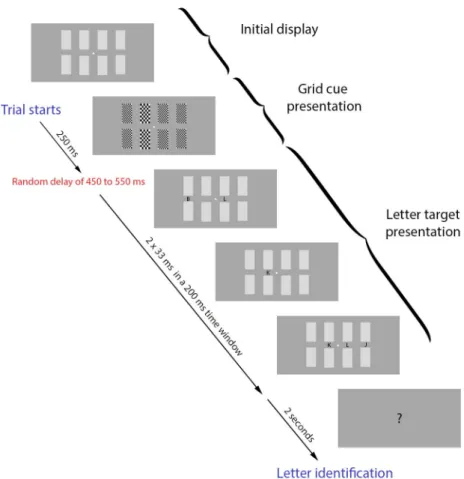
Stimuli were presented on a dark grey background on a cathode-ray tube (60 Hz) using the PsychToolbox-3 implemented in Matlab (Brainard, 1997; Pelli, 1997; Kleiner et al., 2007). A central fixation point was presented during the whole duration of the trial, as well as 8 medium grey squares, symmetrically disposed around the fixation point (4 on each side), forming two lines of four rectangles corresponding to the four locations where the cue and the target letter would appear (vertical gap: 2.05°, horizontal gap: 0.88°) (See Fig.1). Each trial began when the participants pressed the space bar on a keyboard placed in front of them. After 100 ms, the white fixation point turned dark gray for a random duration, ranging from 750 to 1000 ms, indicating that the cue was about to appear. At this point, the eight medium-grey rectangles, representing the four locations (See Fig.1), switched to checkered grids for 250 ms. The grids were composed of either finer or coarser elements. The coarser grid cued the participant to attend to that location. The grids had approximately the same mean luminance as the previous grey field in which half of the pixels were black and half were white, and finer and coarser grids had the same
mean luminance. Following the offset of the cue, there was a random delay of 450 to 550 ms before the onset of the letter sequence, when four letters appeared (one letter per location). Letters were presented independently (i.e., could occur at the same time, or not, with any letter in the other positions) and they randomly flashed twice, each flash lasting for a duration of 33 ms, with a minimum delay of 17 ms between flashes within a time window of 200 ms. The distribution of the random time windows was uniform. The task was to identify the cued letter after a question mark was displayed on the screen 2 seconds after the end of the 200 ms display period. The participants completed two blocks of 300 trials each (600 trials total), and trials for each of the four cued locations occurred in equal numbers (150 at each location) and in random order.
Figure 1. Experiment design (modified Posner task). The grid cues (2nd frame) were presented for 250 ms. Next, each letter was flashed twice (33 ms each time) at random points
EEG acquisition and preprocessing EEG data from 64 active Ag/AgCl electrodes were recorded using a Biosemi Active Two EEG system. EEG was recorded at a sampling frequency of 512 Hz from electrodes mounted on an elastic cap using the International 10-10 System (Sharbrough, Chatrian, Lesser, & Lüders, 1991). Re-referencing of the EEG recording was done offline to the average of the right and left mastoid electrodes. Eye movements and blinks were monitored using horizontal and vertical electrooculography (HEOG/VEOG). A high-pass filter of 0.1 Hz and a low-pass filter of 30 Hz were applied to the EEG signals offline post-recording. The HEOG and VEOG signals were filtered with a high-pass filter of 0.1 Hz and a low-pass filter of 10 Hz. As mentioned above, there were two flashes of each letter, and each one produced a separate ERP. Stimulus-locked ERP events from all trials were epoched in windows ranging from 200 ms pre- stimulus to 800 ms post-stimulus. A baseline correction was performed to the average voltage of the 200 ms pre-stimulus. All epochs containing blinks (VEOG deflection > 50 µV within a time window of 150 ms), eye movements (HEOG deflection > 35 µV within a time window of 300 ms), and other artefacts (signal exceeding ±100 µV) in the EEG signal were excluded from subsequent analysis.
1.1!ERP feature extraction
The feature extraction step consisted of computing the grand average lateralized (Left electrode minus Right electrode) event-related potential (ERP) difference waveforms from 3 electrode pairs (PO7/PO8, O1/O2, and PO3/PO4). This was done by averaging the data with regards to (a) the onset of the attention orientation cue, and (b) the onset of the visual target (letter at the cued location), and further averaging, in each case, the obtained ERP differences over two time windows (early and late, selected on the basis of the grand average waveforms, as detailed below). We chose the time windows used for feature computation based on the ERP literature indicating that the peak of the N2pc component was generally found around 200 ms,
and that the SPCN component was a long lasting component starting around 300 ms. We expected to have a better decoding accuracy by choosing time windows corresponding to the peak of the N2pc component and within the duration of the SPCN component, and by choosing channels of interest (PO7/PO8, O1/O2, PO3/PO4) known to be at or near the peak of the N2pc and SPCN scalp distributions (e.g., Jolicoeur, Brisson, & Robitaille, 2008). These features were computed for each of the four cued locations. This provided a total of 12 features (location Cue and Target [2] x electrode-pair [3] x time window [2]) in each of the 15 participants.
Cue-locked feature computation: For the cue-locked analysis, we computed the lateralized
ERP waves corresponding to each location (1, 2, 3, or 4) for electrodes PO7/PO8, O1/O2, and PO3/PO4 by subtracting the ERP activity measured over the right hemisphere electrode from the ERP activity recorded at the corresponding electrode over the left hemisphere; e.g., PO7 minus PO8. Next, for each location we computed the mean amplitude of the three lateralized ERP measures (PO7/PO8, O1/O2, and PO3/PO4) over two time windows, 170–270 ms and 650–840 ms after cue onset. This provided us with two measures per electrode pair (i.e., 6 features in all). The selection of these time windows was guided by our motivation to have two features (an early and a late one) for lateralized ERP measure. The early time window (170– 270 ms after cue onset) is around at the time we expect to see the N2pc component, that usually starts around 180 ms post-stimulus onset and lasts approximately 100 ms. The late time window (650–840 ms after cue onset), was selected so it would likely be in the time interval of the long lasting SPCN component, which starts at about 300 ms. Importantly, we tried to do the same analysis with small differences concerning the selection of time windows (± 20 ms) and the results were not affected in a significant way, suggesting that the results are robust over variations in the precise parameters of the analysis windows.
for cue-locations 2 and 3, namely a positive difference for the location just left of fixation and a negative difference for the location just right of fixation. This is what we expected if attending to the cued location produced a contralateral negativity. The patterns for the locations further from fixation (locations 1 and 4), were not as clear, in this time window, for reasons we do not understand at the moment and that could be due to the cue or the design of the experiment. The expected contralateral versus ipsilateral patterns were very clear, however, for all locations in the later, SPCN, time window. The expected contralateral versus ipsilateral patterns were very clear, however, for all locations in the later, SPCN, time window. The fact that the patterns of lateralized ERPs were different for different positions in the different time windows, even if not entirely consistent with expectations based on N2pc and SPCN, provides information about which location was cued, which could be used to decode the locus of attention. Unless otherwise stated, these six markers were the cue-locked ERP features we computed for each participant, and that were used to discriminate the four possible locations of the focus of covert attention.
Target-locked feature computation: Signal averaging for target letters was relative to the onset
of the letter presented at the cued location, but otherwise the target-locked features were computed in the same way as the cue-locked ERPs. Different latencies were used for the early and late time windows, however, which set to 0–100 ms and 410–530 ms after target onset, respectively. The selection of these time windows was also guided by our motivation to have an early feature and a late feature that would correspond to an initial sensory response and a later more cognitive response. For target-locked ERPs, we did not expect to see N2pc or SPCN components because attention should already have been deployed at the cued location at the time of target presentation. Thus, we expected that a stimulus appearing at that location would evoke a stronger response than a stimulus at other locations, and that this effect would likely be lateralized. Often, stimuli appearing at a cued location produce a larger contralateral P1. They
also often produce a larger N1, sometimes greater at contralateral electrodes, but also, sometimes larger at ipsilateral electrodes (see Mangun, 1995, and Luck, Fan, & Hillyard, 1993). The waveforms in Figure 2d-f are consistent with a larger contralateral P1 response (visible here in the 0–100 ms period), followed by a later larger contralateral positivity (which we measured between 410 and 530 ms). Note the particularly early P1 is likely a consequence of averaging over two letter onsets, the second of which could be nearly 200 ms later than the first.
1.2!Machine Learning Analysis
In this study, we applied machine learning to address two distinct classification problems. The first and main question was whether we could use lateralized ERPs to decode the locus of attention out of 4 possible locations (i.e., a 4-class decoding problem). The second question used binary classification to discriminate between the neural responses to attended versus unattended stimuli. In both analyses, we explored a number of classification algorithms including linear-discriminant analysis (LDA), k-nearest-neighbor (KNN), and support vector machine (SVM) with either linear or quadratic (RBF) kernels. The results were very similar across the methods, with slightly better results using quadratic SVMs. Hence, the results presented here were computed using quadratic SVMs.
1.2.1!Feature selection
Feature selection was based on the literature of ERP components involved in visual spatial attention (e.g., Jolicoeur, Brisson, & Robitaille, 2008; Mangun 1995). Lateralized ERP waves from electrodes pairs PO7/PO8, PO3/PO4, and O1/O2 (see ERP analysis section) were computed with respect to (i) orientation cue and to (ii) target presentation. These lateralized ERP amplitudes were then averaged over time windows as described in the ERP analysis section above. This led to 12 features (location Cue and Target [2] x electrode-pair [3] x time
1.2.2!Multi-class SVM classification technique
Numerous reports in the literature provide evidence for the high performance of SVM, in particular for high dimensional classification problems (Huang, Davis, & Townshend, 2010; Melgani & Bruzzone, 2004). SVMs were initially designed for binary classification problems. However, a number of strategies have been proposed to embed SVM classifiers in multi-class decoding frameworks. Two of the most widely used approaches for multi-class SVM classification are the One-Against-All (OAA) and the One-Against-One (OAO) approaches. For the purpose of the current study, we used a dendrogram SVM (DSVM), a decision-tree- based multi-SVM classification that has been explored in the machine learning and computer science literature (Bala & Agrawal, 2011; Bennani & Benabdeslem, 2006; Madzarov, Gjorgjevikj, & Chorbev, 2009; Takahashi & Abe, 2002), and has been used recently for the automatic classification of sleep stages (Lajnef et al., 2015). In this framework, a binary SVM is trained at each node of the decision-tree and the optimal hierarchical structure of the decision tree is obtained via hierarchical clustering analysis (HCA). Associating decision tree architecture with binary SVMs combines the advantages of the efficient computation of decision trees and the high classification accuracy of SVMs.
1.2.3!Evaluation of decoding accuracy via cross-validation
The performance of the proposed classification method was evaluated using a Leave-One-Out (LOO) cross-validation procedure. This procedure is a special case of k-fold cross validation, where all individuals except one are used for training, and the classifier is tested on the data from the omitted participant (i.e., on data for which the classifier was not trained). This procedure is repeated as many times as there were participants, each time leaving a different individual out of the training data. Given that we had 15 participants; the procedure was completed in 15 iterations, with each iteration producing either a correct or an incorrect classification of the untrained, test, data set. For example, a decoding accuracy of 66% would
correspond to 10 correct predictions out of 15. The LOO cross-validation method efficiently uses data and provides an asymptotically unbiased estimate of the averaged classification error probability over all possible training sets (Theodoridis & Koutroumbas, 2008).
2.!Results:
2.1!Behavioral results
All 15 participants were able to perform the letter-identification task without difficulty and had a mean accuracy of 95%.
2.2!ERP analysis and feature extraction
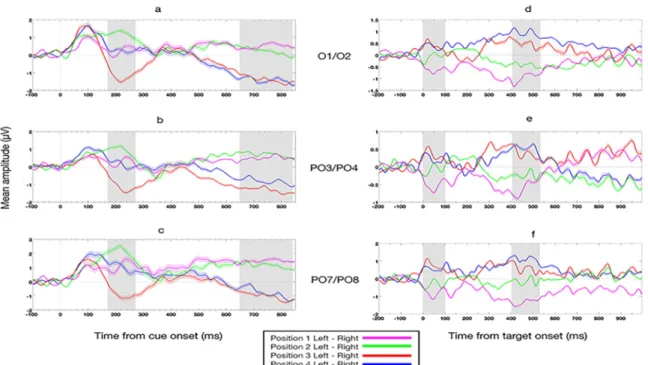
Figure 2 shows the grand average of lateralized cue-locked and target-locked ERP waveforms for the three electrode pairs O1/O2, PO3/PO4, and PO7/PO8, for each of the four cue position (labeled 1 to 4 from left to right). The individual-subject ERPs were used to compute 12 features for each subject, as described in the Method section. As can be seen in Figure 2, the waveforms clearly differentiated the four positions, in the grand averages. The question was whether, and with what spatial accuracy, cue and target locations could be decoded on the basis of individual- subject ERPs
Figure 2. Lateralized ERP waves for electrode pairs PO7/PO8, PO3/PO4, and O1/O2. (a- c) Grand average lateralized (Left electrode minus Right electrode) event-related potential (ERP) difference waveforms, time-locked to the onset of the cue, for the four cue positions (1 to 4 from left to right) for different electrode pairs. (d-f) Same as panels (a-c) but for ERPs locked to the target onset (t=0 at target letter onset). Note the different scales for d-f. Grey rectangles represent the chosen early and late time windows, which were set to be 170–270 ms and 650–840 ms after cue onset and 0–100 ms and 410–530 ms after target onset. The width of the shaded region around each waveform corresponds to the standard error mean (SEM) across the 15 subjects.
2.3!Decoding the locus of attention using SVM classification
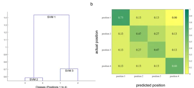
The DSVM technique yielded a 57% correct classification rate when the algorithm was allowed to combine the set of the 12 available features for cue and target locations. Given that this is a four-class decoding problem (4 possible positions), this performance is higher than chance (25%), see also Fig.4 for statistical significance testing of the achieved decoding accuracies. Figure 3 shows the confusion matrix associated with the multi-feature 4-class decoding, with columns indicating predicted locations and rows representing actual locations. The matrix shows that the outermost locations, 1 and 4, were the most easily decoded, with correct identification rates of 73% and 60%, respectively whereas the confusion rate for positions 2 and 3 was 27%. This reflects the fact that discrimination of the spatial location was more difficult when the letter was closer to the center of the display.
For each actual location, the confusion matrix (Fig. 3) indicates what proportion of subjects was correctly classified, and what proportion was incorrectly classified for each of the other three classes. By combining this information with the fact that each location was separated by one letter position, we can compute the mean distance D between the actual and predicted locus of attention for each location:
where !!and "!respectively represent the row and column indices in the confusion matrix, and #$%!the probability of predicting "!when the correct answer is !. On average the mean distance
D between the predicted and the actual focus of attention was 0.62 letter positions. Given the
distance to the display screen, this approximately represents a mean error of 0.55 degrees of visual angle.
The level of classification mentioned above was achieved using a multi-classification framework. In order to determine which features contributed the most to our results, we also computed their decoding accuracy. In other words, we performed 12 single-feature classifications to assess their individual decoding potential (Fig. 4). Here, the probabilistic chance levels (such as 25% in a 4-class decoding problem, or 50% in a 2-class problem) are purely theoretical and are not reliable benchmarks for performance assessments in small sample sizes (Combrisson & Jerbi, 2015). Due to the small sample size, we performed two additional analyses to test the statistical significance of the reported results. The significance thresholds were derived from a binomial distribution function and using permutation testing (Combrisson & Jerbi, 2015)."! Beyond computing decoding accuracy, additional insights into decoding
! !
! !
operating characteristic (ROC) curves. Typically, the area under the ROC curve (AUC) is an attractive measure as it is robust to data imbalance and does not depend on the statistical distribution of the classes. Future analyses of the data presented here may benefit from such metrics.
Figure 3. Structure of the dendrogram SVM framework and mean confusion matrix obtained with multi-feature classification. (a) Dendrogram computed via ascending hierarchical clustering (AHC) shows the multiple SVM taxonomy generated for the four classes (Locations 1 to 4) using the 12 feature space across all 15 subjects. The obtained dendrogram consists of the following 3 binary SVMs. SVM1: [Pos3/Pos4] vs. [Pos1/Pos2], SVM2: [Pos3] vs. [Pos4], and SVM3: [Pos1] vs. [Pos2] (b) Confusion matrix: Each cell shows the proportion a given actual location X (rows) that was classified as being at location Y (columns). The main diagonal therefore represents the proportion of correct classification for each of the 4 locations. Note that the mean of the main diagonal is 57% and corresponds to the overall percentage of correct classification (i.e., decoding accuracy) and that the proportions in each row sum to 1 (within rounding error in the figure), given that all events to be classified are assigned to one of four exclusive categories.
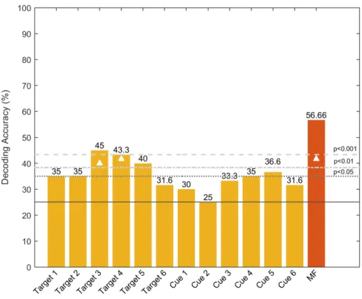
Figure 4. Bar chart of the single-feature decoding accuracy (DA). The features consist of the six target-locked and the six cue-locked lateralized ERPs (3 sites and 2 time-windows). The feature codes on the x-axis indicate whether they were target or cue-locked. The associated number (1-6) indicates whether a given feature was computed in the early (odd number) or late (even number) time window, and from which electrode pair it was computed (1-2: PO7/PO8, 3-4: O1/O2, and 5-6: PO3/PO4). The last (red) bar represents the multi-feature decoding accuracy obtained when we allowed the classifier to combine multiple features. The continuous horizontal line depicts the chance level (25%), while the dotted and dashed lines above it represent the statistical significance thresholds derived for the sample size using the binomial cumulative distribution. The white triangles denote the features with decoding accuracy that exceed the p < .05 level using permutation testing (Combrisson & Jerbi, 2015).
2.4!Binary classification: attended versus non-attended
Using a similar framework, we trained a standard quadratic binary SVM (Cortes & Vapnik, 1995) to determine whether attention was deployed or not at a particular letter location at the time of its presentation. Letters were always presented at various times at each of the four sites. Thus, target-locked ERP analysis can be performed on the presentation of a letter stimulus
with the presentation of a letter at a non-cued location. In other words, the “attended” label corresponds to the condition for which the cue was at the same location as the target (e.g., cue at position 1, target at position 1), and the “non-attended” label corresponds to conditions for which the location of the cue does not match the position of the target (e.g., cue at position 1, target at position 2, 3 or 4). When predicting if a letter/location was attended or non-attended, the decoding accuracy achieved was statistically significant (79 %, p < .001). We then computed the mean decoding accuracy (attended vs. non-attended) for each location separately. The results were statistically significant (p < .05), with a decoding accuracy above 70% for each location separately (see Figure 5).
Figure 5. Bar chart of decoding accuracy for the binary classification - Attended vs Unattended for each of the four locations. The continuous horizontal green line represents the probabilistic chance level (50%), while the dashed and dotted lines above it represent the more reliable sample-size dependent statistical significance thresholds (at p < .01 and p < .05, respectively) using the binomial cumulative distribution. The white stars denote the features with DA that exceed the p < .05 level using permutation testing.
2.5!Ruling out confounding effects from ocular artifacts
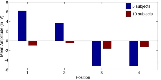
We also examined the relationship between the ERP waveforms and the EOG channels, and found that our results could not be explained by residual eye movements. We computed the lateralized HEOG1/HEOG2 waveforms and separated our total 15 participants in two groups based on the amplitude of their HEOG amplitudes (500 ms following stimulus onset) : group 1 included the 5 participants that moved their eyes the most (n=5) and group 2 included the 10 participants that moved their eyes the least (n=10). As shown in Figure 6, we observed a larger HEOG amplitude in the waveforms computed for group 1 than in those for group 2, which reflects more eye movements.
Figure 6. Bar plot of average HEOG amplitude at 500 ms. Blue bars represent group 1 with the 5 participants that moved their eyes the most (n=5) and red bars represent group 2 with the 10 participants that moved their eyes the least (n=10).
We then applied the multi-class support vector machine (SVM) and the leave-one-out cross- validation framework to evaluate the decoding accuracy (DA) of the 10-participant data subset. The rate of correct prediction obtained was still statistically significant (DA=50%, p < .001,
permutation tests, theoretical chance level 25%). It is therefore highly unlikely that the results are affected by ocular artifacts.
3.!Discussion:
Using a modified Posner cueing task and multi-class SVM, we investigated if lateralized ERP signals could predict the locus of visual spatial attention between four possible locations. In addition, we used the same features, to discriminate attended from non-attended stimuli. Our results showed statistically significant multi-feature decoding (p < .001) using ERPs recorded from occipital and parietal electrodes. This finding shows that the features we used contain class-specific information, and it provides a first step going beyond a simple left-versus-right distinction towards the decoding of a more precise locus of spatial attention using lateralized ERP features.
On the open-ended question of ‘where is attention focused?’ the accuracy of our decoder was above chance and the mean error in localizing the focus of attention was estimated at 0.55 degrees of visual angle (based on the spatial confusion matrix). Moreover, the confusion matrix revealed that locations 1 and 4 were classified with higher precision than locations 2 and 3. Given that locations 2 and 3 were closer to the fixation point at the center of the display, we deduce that there was less information regarding the lateralization of attention for locations 2 and 3. This is perhaps not surprising, given that previous work has relied on strong left-right lateralization (e.g., N2pc, SPCN), and that our stimulus locations were arrayed from left-to- right on the horizontal midline. It is not entirely surprising that the best classification was obtained for the two most extreme locations in the stimulus array. Importantly, however, we
found that we could distinguish between locations within each visual hemifield, indicating that lateralized ERPs can be used to do more than just a global left-right discrimination.
By computing the decoding accuracy for each feature, we found that two features stand out (denoted as Target 03 and Target 04 in Figure 4) and give a decoding accuracy of 45% and 43.3%, respectively, which is better than chance (p < .001). Interestingly, these features correspond to selected time windows (0–100 ms and 410–530 ms after target onset) of the computed lateralized ERP waves at electrodes O1/O2. These results fit nicely with previous work on visual-spatial attention showing both early modulations of sensory responses by attention, as well as modulations of later components on occipital electrodes.
On the more tractable question of whether a presented stimulus is attended or not, our binary SVM classifier led to a prediction accuracy of 79% (p < .001). Moreover, by computing the mean decoding accuracy at each location (1, 2, 3, and 4), we showed that for each individual location we had enough information to determine whether the target was attended or not with accuracy rates of above 70%.
In this study, we focused on the feasibility of using ERPs to predict the location or presence of spatial attention. However, there are other markers of brain activity that might also be used as alternative (or complementary) features. In particular, oscillatory power modulations or long-range interactions may carry critical information with regards to the visuospatial properties of attention deployment. For instance, a previous MEG study has shown the feasibility of decoding covert attention (left vs. right hemifield) using alpha oscillations (van Gerven & Jensen, 2009) and another study showed that electrocorticographic (ECoG) signals recorded from the surface of the brain provide detailed information about shifting of visual attention and its directional orientation in humans (Gunduz et al., 2012).
of new possibilities to determine how neural activity represents the task or stimulus information (Saproo & Serences, 2012). For instance, in vision, it has been successfully used to study object and face perception (Haxby et al., 2001), color vision (Brouwer & Heeger, 2009), and orientation processing (Freeman & Simoncelli, 2011). Many other fields, such as the study of the neural processes underlying reading could also benefit from the development of this approach. The results reported in this study may be considered as another step in this direction. Taken together, the promising findings reported here provide further confirmation that EEG signal contains discriminant features in the time-domain that can be used to decode the locus of visual spatial attention. Furthermore, using a machine learning framework, our results also support the findings of previous work on ERP components and their role in visual spatial attention processing. Although the decoding rates reported are not astounding, they are statistically significant. Moreover, we should emphasize that the displayed letters were located in relatively close proximity (about 1.15 degrees of empty space between letters). Hence, the fact that we could separate such close locations with above-chance accuracy, within visual hemifields, constitutes an important step forward for visuospatial attention decoding. We believe that the methods developed here could be further refined to infer the locus of covert attention in a number of interesting perceptual-cognitive tasks, such as during reading.
A typical ERP component that has been largely used in EEG-based signal classification frameworks is the P300 component (Farwell & Donchin, 1988; Polich, 2007), which is the central feature used in the P300 speller. The P300 is a well known and most widely used paradigm for the visually evoked potential brain computer interface speller, in which characters and numbers are represented in a six-by-six grid (Kaper, Meinicke, Grossekathoefer, Lingner, & Ritter, 2004; Krusienski et al., 2006; Krusienski, Sellers, McFarland, Vaughan, & Wolpaw, 2008). In a nutshell, the underlying principle is that this attention-related response is enhanced when an attended stimulus is flashed. With sufficient repetitions and a smart combination of
flashing entire rows and columns of letters on a screen, the P300 wave becomes a reliable feature that can index the letter (i.e., location on a grid) that is attended. However, it has been argued that the P300-based classification paradigm relies on decoding overt spatial attention, where subjects attend to the intended letter by foveating it ; that is subjects move their gaze towards the target letter (e.g., Brunner et al., 2010). In the present study, we controlled for ocular artifacts using HEOG and VEOG channels to make sure that our signals were not contaminated by eye movements.
Future studies will be needed to increase the spatial resolution and accuracy of the decoded location of covert attention. Such studies may benefit from the inclusion of a wider range of EEG features across the spatial, temporal, and spectral domains, larger sample sizes, and other classification algorithms. As it stands, the current study can be taken as a proof of principle, showing statistically significant discrimination of the location of covert spatial attention using time-domain EEG features from parietal and occipital cortex.
Acknowledgments:
We are grateful to Nicolas Dupuis-Roy suggestions and help in conducting decoding analysis. Support to TL was provided by a fellowship from the PhysNum Lab, part of the Centre de Recherche en Mathématiques (CRM) at Université de Montréal.
This research was funded by grants from the Natural Sciences and Engineering Research Council of Canada to MA and PJ, from infrastructure support from the Fonds de Recherche du Quebec Santé, from research grant 2015-PR-182822 from the Fonds de la Recherche du Québec Nature et Technologies to MA, and from the Canada Research Chairs program to PJ.
References:
Arguin, M., Cavanagh, P., Joanette, Y. (1993). A lateralized alerting deficit in left brain- damaged patients. Psychobiology, 21, 307-323.
Bala, M., & Agrawal, R. K. (2011). Optimal decision tree based multi-class support vector machine. Informatica.
Bennani, Y., & Benabdeslem, K. (2006). Dendogram-based SVM for multi-class classification. CIT Journal of Computing and ….
Bishop, C. M. (2006). Pattern recognition and machine learning.
Blankertz, B., Sannelli, C., Halder, S., Hammer, E. M., Kübler, A., Müller, K.-R., et al. (2010). Neurophysiological predictor of SMR-based BCI performance. NeuroImage,
51(4), 1303–1309. http://doi.org/10.1016/j.neuroimage.2010.03.022
Brouwer, G. J., & Heeger, D. J. (2009). Decoding and reconstructing color from responses in human visual cortex. The Journal of Neuroscience : the Official Journal of the Society for
Neuroscience, 29(44), 13992–14003. http://doi.org/10.1523/JNEUROSCI.3577-09.2009
Brunner, P., Joshi, S., Briskin, S., Wolpaw, J. R., Bischof, H., & Schalk, G. (2010). Does the “P300” speller depend on eye gaze? Journal of Neural Engineering, 7(5), 056013. http://doi.org/10.1088/1741-2560/7/5/056013
Combrisson, E., & Jerbi, K. (2015). Exceeding chance level by chance: The caveat of theoretical chance levels in brain signal classification and statistical assessment of decoding accuracy. Journal of Neuroscience Methods, 250, 126–136.
http://doi.org/10.1016/j.jneumeth.2015.01.010
de Haan, M. (2007). Visual attention and recognition memory in infancy. Infant EEG and
Event-Related Potentials.
Doyle, L. M. F., Yarrow, K., & Brown, P. (2005). Lateralization of event-related beta desynchronization in the EEG during pre-cued reaction time tasks. Clinical
Neurophysiology : Official Journal of the International Federation of Clinical Neurophysiology, 116(8), 1879–1888. http://doi.org/10.1016/j.clinph.2005.03.017
Eimer, M. (1993). Spatial cueing, sensory gating and selective response preparation: an ERP study on visuo-spatial orienting. Electroencephalography and Clinical Neurophysiology,
88(5), 408–420.
Eimer, M. (1996). The N2pc component as an indicator of attentional selectivity.
Electroencephalography and Clinical Neurophysiology, 99(3), 225–234.
http://doi.org/10.1016/0013-4694(96)95711-9
Farwell, L. A., & Donchin, E. (1988). Talking off the top of your head: toward a mental prosthesis utilizing event-related brain potentials. Electroencephalography and Clinical
Freeman, J., & Simoncelli, E. P. (2011). Metamers of the ventral stream. Nature
Neuroscience, 14(9), 1195–1201. http://doi.org/10.1038/nn.2889
Gunduz, A., Brunner, P., Daitch, A., Leuthardt, E. C., Ritaccio, A. L., Pesaran, B., & Schalk, G. (2012). Decoding covert spatial attention using electrocorticographic (ECoG) signals in humans. NeuroImage, 60(4), 2285–2293.
http://doi.org/10.1016/j.neuroimage.2012.02.017
Haxby, J. V., Gobbini, M. I., Furey, M. L., Ishai, A., Schouten, J. L., & Pietrini, P. (2001). Distributed and overlapping representations of faces and objects in ventral temporal cortex. Science (New York, N.Y.), 293(5539), 2425–2430.
http://doi.org/10.1126/science.1063736
Hickey, C., McDonald, J. J., & Theeuwes, J. (2006). Electrophysiological evidence of the capture of visual attention. Journal of Cognitive Neuroscience, 18(4), 604–613. http://doi.org/10.1162/jocn.2006.18.4.604
Huang, C., Davis, L. S., & Townshend, J. R. G. (2010). An assessment of support vector machines for land cover classification. International Journal of Remote Sensing, 23(4), 725–749. http://doi.org/10.1080/01431160110040323
Jolicoeur, P., Brisson, B., & Robitaille, N. (2008). Dissociation of the N2pc and sustained posterior contralateral negativity in a choice response task. Brain Research, 1215, 160– 172. http://doi.org/10.1016/j.brainres.2008.03.059
Jonides, J. (1981). Voluntary vs. automatic control over the mind's eye's movement. In J. B. Long & A. D. Baddeley (Eds.), Attention and performance IX (pp. 187-203). Hillsdale, N J: Erlbaum.
Kaper, M., Meinicke, P., Grossekathoefer, U., Lingner, T., & Ritter, H. (2004). BCI
Competition 2003--Data set IIb: support vector machines for the P300 speller paradigm.
IEEE Transactions on Bio-Medical Engineering, 51(6), 1073–1076.
http://doi.org/10.1109/TBME.2004.826698
Kiss, M., Jolicoeur, P., Dell'acqua, R., & Eimer, M. (2008). Attentional capture by visual singletons is mediated by top-down task set: new evidence from the N2pc component.
Psychophysiology, 45(6), 1013–1024. http://doi.org/10.1111/j.1469-8986.2008.00700.x
Klaver, P., Talsma, D., Wijers, A. A., Heinze, H.-J., & Mulder, G. (1999). An event,related brain potential correlate of visual short,term memory. Neuroreport, 10(10), 2001. Krusienski, D. J., Sellers, E. W., Cabestaing, F., Bayoudh, S., McFarland, D. J., Vaughan, T.
M., & Wolpaw, J. R. (2006). A comparison of classification techniques for the P300 Speller. Journal of Neural Engineering, 3(4), 299–305. http://doi.org/10.1088/1741- 2560/3/4/007
Krusienski, D. J., Sellers, E. W., McFarland, D. J., Vaughan, T. M., & Wolpaw, J. R. (2008). Toward enhanced P300 speller performance. Journal of Neuroscience Methods, 167(1), 15–21. http://doi.org/10.1016/j.jneumeth.2007.07.017
Lajnef, T., Chaibi, S., Ruby, P., Aguera, P.-E., Eichenlaub, J.-B., Samet, M., et al. (2015). Learning machines and sleeping brains: Automatic sleep stage classification using
decision-tree multi-class support vector machines. Journal of Neuroscience Methods, 250, 94–105. http://doi.org/10.1016/j.jneumeth.2015.01.022
Leblanc, E., Prime, D. J., & Jolicoeur, P. (2008). Tracking the location of visuospatial attention in a contingent capture paradigm. Journal of Cognitive Neuroscience, 20(4), 657–671. http://doi.org/10.1162/jocn.2008.20051
Lotte, F., Congedo, M., Lécuyer, A., Lamarche, F., & Arnaldi, B. (2007). A review of classification algorithms for EEG-based brain-computer interfaces. Journal of Neural
Engineering, 4(2), R1–R13. http://doi.org/10.1088/1741-2560/4/2/R01
Luck, S. J. (2005). An introduction to the event-related potential technique.
Luck, S. J., Fan, S., & Hillyard, S. A. (1993). Attention-related modulation of sensory- evoked brain activity in a visual search task. Journal of Cognitive Neuroscience, 5, 188– 195.
Luck, S. J., & Hillyard, S. A. (1994). Spatial filtering during visual search: Evidence from human electrophysiology. Journal of Experimental Psychology. Human Perception and
Performance, 20(5), 1000–1014. http://doi.org/10.1037/0096-1523.20.5.1000
Madzarov, G., Gjorgjevikj, D., & Chorbev, I. (2009). A multi-class SVM classifier utilizing binary decision tree. Informatica.
Mangun, G. R. (1995). Neural mechanisms of visual selective attention. Psychophysiology,
32(1), 4–18.
McCollough, A. W., Machizawa, M. G., & Vogel, E. K. (2007). Electrophysiological
Measures of Maintaining Representations in Visual Working Memory. Cortex; a Journal
Devoted to the Study of the Nervous System and Behavior, 43(1), 77–94.
http://doi.org/10.1016/S0010-9452(08)70447-7
Melgani, F., & Bruzzone, L. (2004). Classification of hyperspectral remote sensing images with support vector machines. Geoscience and Remote Sensing, IEEE Transactions on,
42(8), 1778–1790. http://doi.org/10.1109/TGRS.2004.831865
Müller, H. J., & Rabbitt, P. M. (1989). Reflexive and voluntary orienting of visual attention: Time course of activation and resistance to interruption. Journal of Experimental
Psychology. Human Perception and Performance, 15(2), 315–330.
http://doi.org/10.1037/0096-1523.15.2.315
Müller, K.-R., Tangermann, M., Dornhege, G., Krauledat, M., Curio, G., & Blankertz, B. (2008). Machine learning for real-time single-trial EEG-analysis: From brain–computer interfacing to mental state monitoring. Journal of Neuroscience Methods, 167(1), 82–90. http://doi.org/10.1016/j.jneumeth.2007.09.022