R
OBUST ANDE
FFICIENTM
ESHFREES
OLIDT
HERMO-M
ECHANICSS
IMULATION OFF
RICTIONS
TIRW
ELDINGKirk Fraser, Eng.
Université du Québec à Chicoutimi, UQAC
Thesis presented to l’Université du Québec à Chicoutimi towards the grade of Doctor of Philosophy in Mechanical Engineering
Quebec, Canada
ii Friction stir welding, FSW, is a solid-state joining method that is ideally suited for welding aluminum alloys. Welding of the aluminum is accomplished by way of a hardened steel tool that rotates and is pushed with great force into the work pieces. Friction between the tool and the aluminum causes heat to be generated, which softens the aluminum, rendering it easy to deform plastically. In recent years, the FSW process has steadily gained interest in various fabrication industries. However, wide spread acceptance has not yet been attained. Some of the main reasons for this are due to the complexity of the process and the capital cost to procure the required welding equipment and infrastructure. To date, little attention has been paid towards finding optimal process parameters that will increase the economic viability of the FSW process, thus offsetting the high initial investment most. In this research project, a robust and efficient numerical simulation code called SPHriction-3D is developed that can be used to find optimal FSW process parameters. The numerical method is meshfree, allowing for all of the phases of the FSW process to be simulated with a phenomenological approach. The dissertation starts with a focus on the current state of art. Next an in-depth development of the proposed meshfree formulation is presented. Then, the emphasis turns towards the presentation of various test cases along with experimental validation (the focus is on temperature, defects, and tool forces). The remainder of the thesis is dedicated to the development of a robust approach to find the optimal weld quality, and the associated tool rpm and advancing speed. The presented results are of engineering precision and are obtained with low calculation times (hours as opposed to days or weeks). This is possible, since the meshfree code is developed to run in parallel entirely on the GPU. The overall outcome is a cutting edge simulation approach for the entire FSW process.
Le soudage par friction malaxage, SFM, est une méthode idéale pour relier ensemble des pièces en aluminium. Lors du procédé, un outil en acier très dur tourne à haute vitesse et est presser dans les plaques avec beaucoup de force. L’outil frotte sur les plaques et génère la chaleur, ce qui ramollie l’aluminium, ceci le rendant plus facile à déformé mécaniquement. Récemment, le SFM a connu une croissance de reconnaissance important, par contre, l’industrie ne l’as pas encore adopté unilatéralement. Il existe encore beaucoup de terrain à défricher avant de bien comprendre comment les paramètres du procédé font effet sur la qualité de la soudure. Dans ce travail, on présente une approche de simulation numérique sans maillage pour le SFM. Le code développé est capable de prendre en considération des grandes déformations plastiques, le ramollissement de l’aluminium avec la température, et la condition de frottement complexe. Cette méthode permet de simulé tous les phases du procédé SFM dans une seule modèle. La thèse commence avec un mis en contexte de l’état actuel de la simulation numérique du SFM. Une fois la méthodologie de simulation sans maillage présenté, la thèse concentre sur différents cas de vérification et validation. Finalement, un travail d’optimisation des paramètres du procédé est réalisé avec le code numérique. La méthode de simulation présentée s’agit d’une approche efficace et robuste, ce qui le rend un outil de conception valable pour les ingénieurs qui travaille dans le domaine de SFM.
iv
This work was only possible due to the support and love of my wife, Laurie, my daughter, Kaïla and my son, Alexander.
They are my reason to live, love and continually improve
Success is no accident. It is hard work, perseverance, learning, studying, sacrifice and most of all, love of what you are doing or learning to do.
Pele
Companies have too many experts who block innovation. True innovation really comes from perpendicular thinking.
Peter Diamandis
Effort only fully releases its reward after a person refuses to quit.
vi
A
CKNOWLEDGEMENTS
Firstly, I would like to thank both my research directors, Professor Lyne St-Georges, ing, Ph.D., MBA, and Professor and director of GRIPS, Laszlo I. Kiss, Ph.D. at Université du Quebec a Chicoutimi (UQAC). From the first moment that we met, we have had many thought-provoking and motivating discussions. Their support and belief in my ability as an engineer and researcher helped me to achieve all the goals set out at the start of the project. Without their unwavering support and guidance, I would not have endeavoured to enter into the PhD program. They provided a positive and nurturing learning environment that was elemental to the success of the project. I would also like to deeply thank the support and friendship of George Laird, Ph.D., PE, and owner of Predictive Engineering. I cherish the more than 10 years that we have known each other and the many interesting and stimulating engineering projects that we have completed together. George’s support of my Ph.D. project has been a key factor in its success. His give it all, 110% attitude has been an inspiration in not only my engineering work, but also my life in general.
Over the last decade, I have had the opportunity to work with many encouraging and supportive engineers and technicians. My time at AP-Dynamics gave me a strong foundation as a numerical simulation engineer. Mario Forcinito, P.Eng., Ph.D., and Paul Alves, P.Eng, M.Sc., owners of AP-Dynamics, instilled a strong interest in achieving personal excellence and more importantly, a perceived need to continually improve myself and the team that I work with. I would not have considered embarking in the doctoral program without their mentoring at the early stage of my career. I would also like to thank the many colleagues at CPI Proco and Roche.
The successful completion of a Ph.D. project requires an extensive support staff. I would like to thank all the technicians that have helped to make the research work possible. Special thanks go out to Alexandre Morin, Université du Quebec a Chicoutimi (UQAC), for his dedication and continued help preparing the experiments, maintaining the equipment, and operating the FSW equipment. I would also like to thank the help of Alexandre Maltais, CSFM-UQAC, for his help with performing various industry scale FSW tests. I also would like to extend my gratitude to my fellow researchers and colleagues at Université du Quebec a Chicoutimi (UQAC) for their help with many different aspects of the research project.
Undertaking and completing a doctorate requires a certain mindset and attitude. I would like to thank my mom, Donna Fraser, and my Dad, Ian Fraser, for instilling in me at an early age, the drive to give my best in everything I do. Words are not enough to express my gratitude for the time and dedication that they expended in raising me to be a strong and independent person. Who I am today is in direct reflection of whom they raised me to be. I would also like to extend further appreciation towards the in depth interest that my Dad took in my research work. The countless hours spent creating a graphical user
interface for the simulation code, as well as the extensive time reviewing and correcting each and every one of my reports, articles, and this dissertation.
Over the course of my doctoral research project, I was lucky enough to receive numerous grants and scholarships. I would like to extend my warmest appreciation towards Fonds de recherche Nature et technologie du Quebec (FRQNT) for providing a generous scholarship. I would like to thank Rio-Tinto-Alcan for awarding me with the bourses du groupe de produits Aluminium de Rio Tinto. Also, thanks to the Fondation de l’UQAC (FUQAC), Bombardier (bourse Fondation J. Armand Bombardier), INALCO, and UQAC PAIR for their generous scholarships.
I would also like to thank NVIDIA for their donation of a GTX Titan Black GPU for the research work. I would like to acknowledge the support from The Portland Group (PGI) for providing a licence for the PGI CUDA Fortran compilers. Also, thanks to the Centre de recherche sur l’aluminium – REGAL for generously providing funds for my participation in the 13th International LS-DYNA Conference, The 4th International Particles Conference, and the 11th International FSW Symposium. Without these generous contributions, the research project would not have been possible.
Finally, and most importantly, I would like to thank my best friend for her boundless and unconditional support and love. Her incredible gift for mathematics and strategy were major driving forces to complete my undergraduate degree and to take on the challenges of a Ph.D. She is a beautiful person, an incredible mother, and the love of my life.
Saguenay, Quebec, April , 2017 Kirk Fraser, Eng.
viii
C
ONTENTS
1
INTRODUCTION ... 1
1.1 Problem Statement ... 3
1.2 Research Project Objectives ... 3
1.3 Major Developments in this Project ... 4
1.4 Thesis Layout ... 5
1.5 A Note on Notation ... 7
2
CURRENT STATE OF THE ART ... 9
2.1 Solid-State Joining Processes ... 10
2.1.1 Linear Friction Welding ... 10
2.1.2 Rotary Friction Welding ... 11
2.1.3 Explosion Welding ... 12
2.2 FSW Process ... 12
2.2.1 0a – Clamping ... 15
2.2.2 0b - Tool approach ... 15
2.2.3 0c - Initial tool contact... 16
2.2.4 1 - Plunge ... 16
2.2.5 2 - Dwell... 17
2.2.6 3 - Advance ... 17
2.3 FSW Variants ... 18
2.4 Common FSW Defects ... 21
2.5 Fluid or Solid Formulation ... 23
2.6 Numerical Methods ... 24
2.6.1 Mesh (Grid) Based Methods ... 25
2.6.2 Meshfree Methods Requiring a Background Mesh ... 27
2.6.3 Meshfree Methods Not Requiring a Background Mesh (True Meshfree) ... 28
2.7 Material Models ... 29
2.8 Friction and Contact Behaviour ... 33
2.9 FSW Process Parameter Optimization ... 36
2.10 Mass and Time Scaling ... 37
3
METHODOLOGY ...39
3.1 Continuum Mechanics for FSW ... 40
3.2 The Smoothed Particle Method ... 44
3.2.1 Discrete Interpolation ... 45
3.2.2 Smoothing Functions... 47
3.3 Solid Mechanics Approach For FSW ... 52
3.3.1 Equation of State for Weakly Compressible Material ... 53
3.3.2 Thermal Expansion ... 55
x
3.3.4 Radial Return Plasticity ... 56
3.4 SPH Form of the Continuum Equations ... 59
3.4.1 Conservation of Mass ... 59
3.4.2 Conservation of Momentum ... 60
3.5 SPH Form of the Constitutive Equations ... 62
3.5.1 Strain Rate Tensor ... 62
3.5.2 Spin Tensor ... 62
3.5.3 Jaumann Rate Equation ... 63
3.6 Artificial Viscosity... 63
3.7 Velocity Averaging using the XSPH Approach ... 64
3.8 Some Common issues with the Smoothed Particle Method ... 65
3.8.1 Completeness and Consistency ... 65
3.8.2 Tensile Instability – Artificial Stress ... 68
3.9 Heat Transfer ... 70
3.9.1 Plastic Work ... 73
3.9.2 Friction Work ... 74
3.9.3 Finding the Free Surface Elements ... 75
3.9.4 Visualizing Heat Flux Vectors ... 77
3.9.5 Surface Convection ... 79
3.9.6 Surface Radiation ... 81
3.10 FKS Flow Stress Model ... 81
3.10.2 Strain Hardening Effect ... 86
3.10.3 Strain Rate Effect ... 86
3.10.4 Thermal Softening Effect ... 87
3.10.5 The Flow Stress Model ... 87
3.10.6 Iterative Plasticity ... 91
3.11 SPH-FEM Hybrid ThermoMechanical Contact ... 91
3.11.1 Contact Pair Bucket Sort ... 93
3.11.2 Node to Surface Contact Detection ... 95
3.11.3 Mechanical Contact Formulation ... 99
3.11.4 Thermal Contact Approach ... 102
3.12 Cumulative Damage Friction Model ... 105
3.12.1 The Stick-Slip Friction Model ... 106
3.12.2 The Contact Interface ... 107
3.12.3 Idealization of the Contact Interface with a Cumulative Damage Model ... 108
3.12.4 Cumulative Damage Friction Force Equation... 109
3.13 Pin Thread and Shoulder Scroll Model ... 110
3.14 Tool Wear Prediction ... 113
3.15 Solution Procedure ... 114
4
PARALLEL PROGRAMMING ... 119
4.1 GPU Architecture ... 120
xii
4.2.1 Memory ... 125
4.2.2 CUDA Kernels ... 126
4.3 Parallelization Strategy of the SPH Code ... 128
4.3.1 Neighbor List Data Structure ... 128
4.3.2 Structure of Arrays (SoA) ... 130
4.3.3 SPH Sums (Reductions)... 131
4.4 Performance Comparison – Heat Transfer Simulation ... 132
4.4.1 Performance Results ... 133
4.5 Adaptive Neighbor Search On the GPU ... 135
4.6 An Efficient Parallel Surface Triangulation Algorithm ... 138
5
MODELLING, VALIDATION AND TEST CASES ... 140
5.1 Butt Joint Weld – Friction Stir Weld ... 141
5.1.1 Model Description... 145
5.1.2 Simulation Results – Material Model Testing ... 151
5.1.3 Simulation Results - Friction Model Testing ... 156
5.1.4 Simulation Results - Process Parameter Testing ... 157
5.2 Lap Joint - Friction Stir Spot Weld ... 161
5.2.1 Model Description... 164
5.2.2 Simulation Results ... 166
5.3 Complex Joint Geometry ... 168
5.3.2 Simulation Results ... 172
5.4 Hollow Core Joint - Bobbin Tool ... 182
5.4.1 Model Description... 184
5.4.2 Simulation Results ... 185
5.5 Parametric Test Cases ... 189
5.5.1 Smoothing length scale factor ... 191
5.5.2 Smoothing function ... 192
5.5.3 Velocity Scaling Factor... 195
5.5.4 CFL Number ... 197
5.5.5 XSPH ... 199
5.5.6 Thread Pitch ... 200
5.5.7 Support Base Material ... 203
5.6 Cooling and Distortion of a Butt Joint Weld ... 206
5.6.1 Model Description... 206
5.6.2 Digital Image Correlation ... 211
5.6.3 Residual Stress Results ... 214
6
PROCESS PARAMETER OPTIMIZATION ... 216
6.1 Weld Quality Metrics ... 218
6.1.1 Defect Metric ... 219
6.1.2 Mixing Metric... 222
6.1.3 Maximum Temperature Metric ... 224
6.1.4 Moving Thermo-Couple Variation Metric ... 225
xiv
6.1.6 Overall Weld Quality ... 228
6.2 Weld Quality Results ... 229
6.2.1 Defects ... 229
6.2.2 Experimental Validation of Simulated Defects ... 232
6.2.3 Mixing ... 236
6.2.4 Max Temperature and MTC1 Variation ... 240
6.2.5 Tool Wear ... 244
6.2.6 Overall Weld Quality ... 247
6.3 Response Surface Construction ... 248
6.3.1 Results ... 250
6.4 Optimization - Maximizing overall Weld Quality ... 252
6.5 Optimization - Minimizing Defects ... 256
6.6 Optimization - Maximizing Advance Speed Based on Weld Quality ... 258
7
CONCLUSIONS AND OUTLOOK... 264
8
REFERENCES ... 268
9
APPENDICES ... 286
USEFUL FORMULAE ... 287
VERIFICATION CASE - BEAM WITH FIXED ENDS ... 292
VERIFICATION CASE - ELASTIC VIBRATION OF AN ALUMINUM CANTILEVER BEAM ... 296
VERIFICATION CASE - ELASTIC-PLASTIC TENSILE TEST ... 299
VERIFICATION CASE - ELASTIC-PLASTIC COMPRESSION TEST WITH HEAT GENERATION ... 302
CONVECTION AS A SURFACE INTEGRAL ... 309
FULL IMPLICIT SMOOTHED PARTICLE METHOD (FISPM) ... 310
xvi
L
IST OF
T
ABLES
TABLE 3-1–DIMENSIONAL SPECIFIC SMOOTHING CONSTANTS ... 51
TABLE 3-2–CONSTANTS USED FOR PROPOSED FLOW STRESS MODEL ... 89
TABLE 3-3–CUMULATIVE DAMAGE CONSTANTS USED FOR PROPOSED FRICTION MODEL ... 108
TABLE 5-1–THERMAL-PHYSICAL PROPERTIES SIMULATION MODEL COMPONENTS ... 150
TABLE 5-2–JOHNSON-COOK PARAMETERS –AA6061-T6 ... 150
TABLE 5-3–TEMPERATURE COMPARISON AT END OF DWELL PHASE (TC9) ... 152
TABLE 5-4–MAXIMUM TEMPERATURE COMPARISON DURING ADVANCE PHASE (TC4) ... 152
TABLE 5-5–MAXIMUM TEMPERATURE COMPARISON DURING ADVANCE PHASE (TC4) ... 158
TABLE 5-6–THERMOPHYSICAL PROPERTIES OF AA6005-T6 ... 171
TABLE 5-7-MATERIAL FLOW COMPARISON BETWEEN EXPERIMENT AND SIMULATION ... 188
TABLE 5-8–THERMAL PROPERTIES OF BASE MATERIALS USED IN TEST CASE ... 203
TABLE 5-9–MATERIAL PROPERTIES USED IN COOLING ANALYSIS ... 207
TABLE 6-1–OPTIMIZATION STUDY PROCESS PARAMETERS ... 217
TABLE 6-2–WELD QUALITY METRICS ... 228
TABLE 6-3–COMPARISON OF DEFECT SURFACE AREA BETWEEN EXPERIMENT AND SIMULATION... 233
TABLE 6-4–RESPONSE SURFACE COEFFICIENT RESULTS ... 250
TABLE 6-5–WELD QUALITY OPTIMIZATION RESULTS ... 255
TABLE 6-7–ADVANCING SPEED OPTIMIZATION RESULTS ... 262
LIST OF FIGURES
FIGURE 1-1–A HAFTED TOOL [1] ... 1FIGURE 1-2–FSW PROCESS [2] ... 2
FIGURE 2-1–LINEAR FRICTION WELDING PHASES [4] ... 10
FIGURE 2-2–TURBINE ASSEMBLED BY LINEAR FRICTION WELDING [4] ... 11
FIGURE 2-3–ROTARY FRICTION WELDING [3]... 11
FIGURE 2-4–EXPLOSION WELDING PROCESS (ADAPTED FROM [18])... 12
FIGURE 2-5–FSW PROCESS PARAMETERS AND TOOL GEOMETRY [25,26] ... 13
FIGURE 2-6–FSW PROCESS PHASES [29] ... 14
FIGURE 2-7–BOBBIN TOOL PROCESS [55] ... 19
FIGURE 2-8–FSSW PROCESS [66] ... 19
FIGURE 2-9–REFILL FSW PROCESS [75]... 20
FIGURE 2-10–TWIN STIRTM PROCESS [89] ... 21
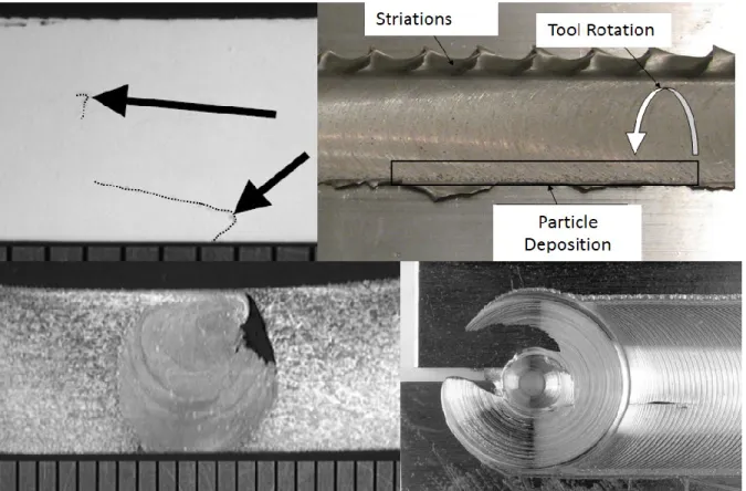
FIGURE 2-11–COMMON DEFECTS IN FSW WELDS –TOP LEFT:LAZY S OR KISSING BOND; TOP RIGHT:FLASH AND PARTICLE DEPOSITS; BOTTOM LEFT:WORMHOLE; BOTTOM RIGHT:SURFACE DEFECT ... 22
FIGURE 2-12–MACROGRAPH OF GROOVE PATTERN IN FSW WELD TRACK ... 23
FIGURE 2-13–FLOW STRESS MODEL USED BY DIALAMI ET AL.[107] ... 30
FIGURE 2-14–HANSEL-SPITTEL MODEL FOR AA6061-T6–ASSIDI ET AL.[139] ... 31
xviii
FIGURE 2-16–TEMPERATURE DEPENDENT INITIAL YIELD ... 33
FIGURE 3-1–CONTINUUM DESCRIPTION ... 41
FIGURE 3-2–INTERPOLATION IN SPH METHOD ... 44
FIGURE 3-3–COMPARISON OF SMOOTHING FUNCTION WITH 2R SUPPORT ... 50
FIGURE 3-4–COMPARISON OF SMOOTHING FUNCTION DERIVATIVES WITH 2R SUPPORT ... 51
FIGURE 3-5–COMPARISON OF LINEAR AND GRUNEISEN EOS ... 54
FIGURE 3-6–SCHEMATIC OF THE UPDATE OF THE YIELD STRESS ... 57
FIGURE 3-7-SCHEMATIC OF THE UPDATE OF THE YIELD STRESS ... 59
FIGURE 3-8–INCOMPLETE INTERPOLATION (ADAPTED FROM XU [207]) ... 65
FIGURE 3-9–INCOMPLETE INTERPOLATION EXAMPLE... 66
FIGURE 3-10–CORRECT DENSITY FIELD WITH RE-NORMALIZATION APPROACH ... 67
FIGURE 3-11–TENSILE INSTABILITY ... 68
FIGURE 3-12–TENSILE INSTABILITY REMOVED ... 70
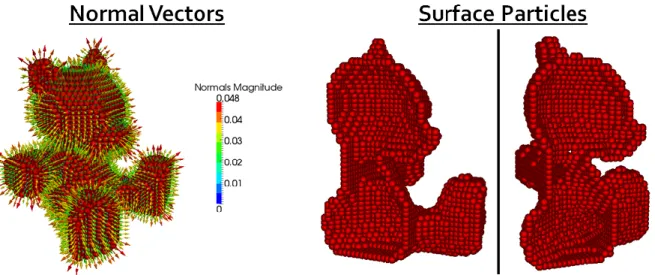
FIGURE 3-13–NORMAL VECTORS AND SURFACE PARTICLES –LEFT:NORMAL VECTORS; RIGHT:FREE SURFACE PARTICLES ... 77
FIGURE 3-14–HEAT FLUX VECTORS ... 78
FIGURE 3-15–SURFACE CONVECTION BOUNDARY CONDITION ... 79
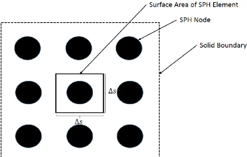
FIGURE 3-16–EQUIVALENT SURFACE AREA OF AN SPH ELEMENT ... 80
FIGURE 3-18–TEMPERATURE COMPARISON AT CENTER OF SPECIMEN FOR Ε= 1.0 ... 83
FIGURE 3-19–THERMOCOUPLE COMPARISON DURING COMPRESSION TESTING (Ε= 0.001,T=150°C) ... 83
FIGURE 3-20–COMPRESSION TEST RESULTS: Ε= 0.001 ... 84
FIGURE 3-21-COMPRESSION TEST RESULTS: Ε= 1.0... 85
FIGURE 3-22-COMPRESSION TEST RESULTS: Ε= 10.0 ... 85
FIGURE 3-23–FINAL SHAPE OF THE COMPRESSED CYLINDERS (Ε= 0.001) ... 86
FIGURE 3-24–FKS FLOW STRESS SURFACE,𝜎𝑦(𝜀𝑝, 𝑇) UPPER,𝜎𝑦(𝜀, 𝑇) ... 88
FIGURE 3-25–COMPARISON OF THE YIELD VALUES ... 89
FIGURE 3-26–COMPRESSION TEST RESULTS FOR STRAIN RATE 0.001,1.0,10.0, AND 100.0 ... 90
FIGURE 3-27–CONTACT EXAMPLE ... 92
FIGURE 3-28–NODE TO SURFACE CONTACT... 93
FIGURE 3-29–EMBEDDED SPHERES IN TRIANGULAR FINITE ELEMENT MESH ... 94
FIGURE 3-30–DETERMINING THE RADIUS OF THE EMBEDDED SPHERE ... 95
FIGURE 3-31–CONTACT DETECTION ... 96
FIGURE 3-32–CONTACT POINT INSIDE OR OUTSIDE OF FINITE ELEMENT ... 98
FIGURE 3-33–SPRING AND DAMPER CONTACT MODEL ... 100
FIGURE 3-34–HYBRID THERMO-MECHANICAL CONTACT EXAMPLE ... 103
FIGURE 3-35–FULL NEIGHBORS LIST (NEIB)... 104
xx
FIGURE 3-37–THERMAL PROBLEM NEIGHBORS (𝑁𝑒𝑖𝑏𝑇ℎ𝑒𝑟𝑚) ... 105
FIGURE 3-38–POTENTIAL CONTACT PAIRS NEIGHBOR (𝑁𝑒𝑖𝑏𝐶𝑜𝑛𝑡𝑎𝑐𝑡) ... 105
FIGURE 3-39–WELD SURFACE OF A FSW JOINT ... 106
FIGURE 3-40–ASPERITY EVOLUTION WITH RELATION TO SLIP RATIO ... 107
FIGURE 3-41–EVOLUTION OF THE SLIP RATIO AS A FUNCTION OF SURFACE DAMAGE ... 109
FIGURE 3-42–TYPICAL MESH DENSITY IN A THREADED TOOL CFD SIMULATION MODEL [229] ... 111
FIGURE 3-43–EQUIVALENT TOOL MODEL WITHOUT THREADS ... 111
FIGURE 3-44–EQUIVALENT THREAD FORCE MODEL... 112
FIGURE 3-45–TOOL WEAR PREDICTION EXAMPLE ... 114
FIGURE 4-1–GPU ARCHITECTURE ... 121
FIGURE 4-2–CODE COMPARISON BETWEEN FORTRAN AND CUDAFORTRAN ... 123
FIGURE 4-3–GPUARCHITECTURE (RUETSCH AND FATICA [250]) ... 124
FIGURE 4-4–SOFTWARE AND HARDWARE SCHEMATIC (NVIDIA,[268]) ... 124
FIGURE 4-5–HOST AND DEVICE MEMORY SCHEMATIC (BALFOUR [212]) ... 125
FIGURE 4-6–NEIGHBOR ARRAY LAYOUT,NEIB(NTOTAL,NNEIB_MAX) ... 130
FIGURE 4-7–AOS AND SOA DATA STRUCTURES ... 131
FIGURE 4-8–SPH SUM EXAMPLE ... 132
FIGURE 4-9–TOTAL SIMULATION TIME COMPARISON... 134
FIGURE 4-11–SCHEMATIC OF CELL SEARCH METHOD ... 135
FIGURE 4-12–SURFACE TRIANGULATION SEQUENCE... 139
FIGURE 5-1–EXPERIMENTAL SETUP FOR BUTT WELD JOINT ... 142
FIGURE 5-2–THERMOCOUPLE ARRANGEMENT FOR BUTT WELD JOINT ... 143
FIGURE 5-3–FSW TOOL FOR BUTT WELD JOINT... 144
FIGURE 5-4–TYPICAL TEMPERATURE HISTORY FOR BUTT WELD JOINT ... 145
FIGURE 5-5–FSW MODEL OF BUTT WELD JOINT ... 146
FIGURE 5-6–FLOW STRESS FROM JC-FKS(FROM EQN.(5-1)) COMPARED TO COMPRESSION TEST ... 148
FIGURE 5-7–THERMAL PROPERTIES OF AA6061-T6... 149
FIGURE 5-8–TEMPERATURE HISTORY FOR CASE 1A,1B,1C, AND 1D ... 152
FIGURE 5-9–COMPARISON OF PREDICTED DEFECTS (ADVANCING SIDE OF CASE 1C AND 3C) TO EXPERIMENT ... 153
FIGURE 5-10–TORQUE AND FORGE FORCE COMPARISON FOR CASE 1A,1B,1C, AND 1D ... 154
FIGURE 5-11–THERMAL CAMERA IMAGE AT END OF WELD FOR 800 RPM 1069 MM/MIN –LEFT:SIMULATION CASE 1C;RIGHT:EXPERIMENT WITH THERMAL CAMERA.TEMPERATURE IN [°C], SAME SCALE BOTH IMAGES. 154 FIGURE 5-12–TEMPERATURE (°C), PLASTIC STRAIN, AND INTERNAL DEFECTS FOR CASES 1A,1B,1C, AND 1D ... 155
FIGURE 5-13–TEMPERATURE HISTORY FOR CASE 2A,2B,2C, AND 2D ... 156
FIGURE 5-14–TORQUE AND FORGE FORCE COMPARISON FOR CASE 2A,2B,2C, AND 2D ... 157
xxii FIGURE 5-16-TORQUE AND FORGE FORCE COMPARISON FOR CASE 3A,3B, AND 3C ... 159
FIGURE 5-17-COMPARISON OF PREDICTED DEFECTS (ADVANCING SIDE OF CASE 3A) TO EXPERIMENT ... 159
FIGURE 5-18-COMPARISON OF PREDICTED DEFECTS (ADVANCING SIDE OF CASE 3B) TO EXPERIMENT ... 160
FIGURE 5-19–COMPARISON OF PREDICTED DEFECTS (ADVANCING SIDE OF CASE 1C AND 3C) TO EXPERIMENT
... 160
FIGURE 5-20–COMPARISON OF TOOL WEAR FOR CASES 3A,3B, AND 3C ... 161
FIGURE 5-21– FSSW EXAMPLES; ALUMINUM TRAIN ROOF [286] (LEFT), ALUMINUM CAR DOOR PANEL [287]
(RIGHT) ... 162
FIGURE 5-22–FSSW EXPERIMENTAL SETUP ... 163
FIGURE 5-23–CEE-UQACFSW MACHINE... 164
FIGURE 5-24–FSSW SIMULATION MODEL... 165
FIGURE 5-25–FINISHED WELDS:800 RPM (LEFT),1000 RPM (CENTER),1200 RPM (RIGHT)... 166
FIGURE 5-26–FSSW TEMPERATURE COMPARISON FOR THE THREE CASES ... 167
FIGURE 5-27–FORGE FORCE (LEFT) AND SPINDLE TORQUE (RIGHT) COMPARISON ... 167
FIGURE 5-28–FLASH AND PLASTIC STRAIN COMPARISON –TOP:CASE 1-800 RPM;MIDDLE:CASE 2-1000 RPM;BOTTOM:CASE 3-1200 RPM ... 168
FIGURE 5-29–COMPLEX JOINT ... 169
FIGURE 5-30–FSW JOINT SIMULATION MODEL ... 170
FIGURE 5-31-TEMPERATURE AND DEFORMATION RESULTS FOR THE THREE CASES ... 174
FIGURE 5-33-TEMPERATURE HISTORY RESULTS FOR THE THREE CASES ... 176
FIGURE 5-34-SPINDLE TORQUE AND FORGE FORCE COMPARISON ... 177
FIGURE 5-35-FLASH HEIGHT COMPARISON AT END OF ADVANCING PHASE ... 177
FIGURE 5-36-PLASTIC STRAIN AT END OF ADVANCING PHASE SHOWING THE EFFECTIVE WELD ZONE ... 178
FIGURE 5-37–INITIAL PARTICLE POSITIONS USED IN PATH LINE ANALYSIS... 180
FIGURE 5-38–PARTICLE PATH LINES FOR THE THREE CASES ... 181
FIGURE 5-39–MIXING RESULTS FOR THE THREE CASES... 182
FIGURE 5-40–BOBBIN TOOL AND SIMULATION MODEL ... 185
FIGURE 5-41–BOBBIN FSW SPINDLE TORQUE ... 186
FIGURE 5-42–BOBBIN FSW TEMPERATURE (LEFT) AND MIXING RESULTS (RIGHT) ... 187
FIGURE 5-43–COMPARISON OF PREDICTED AND EXPERIMENTAL DEFECTS ... 188
FIGURE 5-44–BOBBIN TOOL WEAR PREDICTION FROM SIMULATION MODEL ... 189
FIGURE 5-45 – COMPARISON OF THE TEMPERATURE FIELD AND DEFECT PREDICTION; ℎ𝑠𝑐𝑎𝑙𝑒 = 1.1 (LEFT), ℎ𝑠𝑐𝑎𝑙𝑒 = 1.2(CENTER), ℎ𝑠𝑐𝑎𝑙𝑒 = 1.3(RIGHT) ... 192
FIGURE 5-46-RUNTIME COMPARISON FOR THE SMOOTHING LENGTH SCALE FACTOR TEST ... 192
FIGURE 5-47–COMPARISON OF SYSTEM ENERGIES FOR THE SMOOTHING FUNCTION TEST:KINETIC ENERGY (TOP LEFT), INTERNAL ENERGY (TOP RIGHT), CONTACT ENERGY (BOTTOM LEFT), AND ENERGY RATIO (BOTTOM RIGHT) ... 193
FIGURE 5-48-COMPARISON OF SMOOTHING FUNCTION DERIVATIVES WITH 2R SUPPORT (REPEAT OF FIGURE 3-4 FOR CLARITY) ... 195
xxiv FIGURE 5-49–AVERAGE DEFECT HEIGHT CONVERGENCE AS A FUNCTION OF VELOCITY SCALING FACTOR ... 196
FIGURE 5-50-RUNTIME COMPARISON FOR THE VELOCITY SCALING FACTOR ... 196
FIGURE 5-51–COMPARISON OF KINETIC TO INTERNAL ENERGY RATIO FOR THE VELOCITY SCALING TEST .... 197
FIGURE 5-52–RUNTIME COMPARISON FOR THE CFL NUMBER TEST ... 198
FIGURE 5-53-COMPARISON OF SYSTEM ENERGIES FOR THE CFL TEST:KINETIC ENERGY (TOP LEFT), INTERNAL ENERGY (TOP RIGHT), CONTACT ENERGY (BOTTOM LEFT), AND ENERGY RATIO (BOTTOM RIGHT) ... 199
FIGURE 5-54–DEFECT VOLUME COMPARISON FOR THE XSPH TEST CASE:𝜁𝑋𝑆𝑃𝐻 = 0.05(TOP LEFT),𝜁𝑋𝑆𝑃𝐻 =
0.10(TOP RIGHT),𝜁𝑋𝑆𝑃𝐻 = 0.15(BOTTOM LEFT),𝜁𝑋𝑆𝑃𝐻 = 0.20(BOTTOM RIGHT) ... 200
FIGURE 5-55–CROSS SECTION CUT THROUGH THICKNESS OF WORK PIECES:𝑝𝑡ℎ𝑟𝑒𝑎𝑑 = 0(TOP),𝑝𝑡ℎ𝑟𝑒𝑎𝑑 =
0.8𝑚𝑚(CENTER), AND 𝑝𝑡ℎ𝑟𝑒𝑎𝑑 = 1.25 MM (BOTTOM) ... 202
FIGURE 5-56–DEFECT PREDICTION COMPARISON:𝑝𝑡ℎ𝑟𝑒𝑎𝑑 = 0(TOP LEFT),𝑝𝑡ℎ𝑟𝑒𝑎𝑑 = 0.8 MM (TOP RIGHT), AND 𝑝𝑡ℎ𝑟𝑒𝑎𝑑 = 1.25 MM (BOTTOM) ... 202
FIGURE 5-57– COMPARISON OF THE TEMPERATURE AND DEFECT RESULTS FOR THE BASE MATERIAL TEST: SURFACE TEMPERATURE (TOP ROW), INTERNAL DEFECTS (MIDDLE ROW), AND CROSS SECTION TEMPERATURE (BOTTOM ROW) ... 204
FIGURE 5-58–SUPPORT BASE MATERIAL POWER COMPARISONS ... 205
FIGURE 5-59–SUPPORT BASE MATERIAL INPUT POWER COMPARISONS ... 206
FIGURE 5-60– INITIAL CONDITIONS AT START OF COOLING ANALYSIS (CLOCKWISE FROM TOP LEFT):MIXING RESULTS IN THE WELD ZONE, TEMPERATURE DISTRIBUTION (°C), EFFECTIVE STRESS (PA), SURFACE PARTICLES ... 208
FIGURE 5-62–TEMPERATURE PROFILES (LEFT TO RIGHT): T =24 S,32 S,105 S, AND 524 S (FINAL STEP) . 210
FIGURE 5-63–TEMPERATURE HISTORY FOR TC1,TC3,TC4, AND TC6 ... 211
FIGURE 5-64–ARAMIS EXAMPLES (FROM GOM’S WEBSITE, SEE ABOVE TEXT) ... 211
FIGURE 5-65–DIGITAL IMAGE CORRELATION SETUP ... 212
FIGURE 5-66–PRE-WELD SETUP FOR DIC SHOWING PAINTED WORK PIECES, THERMOCOUPLES AND SUPPORT STRUCTURE... 213
FIGURE 5-67–RESIDUAL STRESS RESULTS FROM FSW EXPERIMENT USING DIC ... 214
FIGURE 5-68–PREDICTED RESIDUAL STRESS FROM SPH MODEL ... 214
FIGURE 6-1–WELD-QUALITY MEASURING ZONE USED FOR THE METRIC CALCULATIONS (SHOWN IN BLUE AND GREEN) ... 219
FIGURE 6-2–DEFECT MEASURED FROM THE PREDICTED FREE-SURFACE ELEMENTS ... 220
FIGURE 6-3–SURFACE TRIANGULATION OF THE INTERNAL DEFECTS ... 220
FIGURE 6-4–INCREASED SURFACE AREA IN WELD TRACK... 221
FIGURE 6-5–FLASH PREDICTION CONTRIBUTING TO DEFECT METRIC ... 222
FIGURE 6-6–QUANTIFICATION OF WORK PIECE MIXING ... 223
FIGURE 6-7–PLASTIC STRAIN THROUGHOUT THE THICKNESS OF THE WELDED PLATES ... 224
FIGURE 6-8–TYPICAL TEMPERATURE CONTOURS ... 224
FIGURE 6-9 – LOCATION OF MTC1 AND A THROUGH HOLE METHOD FOR MOUNTING THE THERMOCOUPLE
(ADAPTED FROM [299]) ... 226
xxvi FIGURE 6-11–COMMON TOOL WEAR BEHAVIOUR [300] ... 227
FIGURE 6-12–DEFECT METRIC COMPARISON AT END OF ADVANCE PHASE ... 229
FIGURE 6-13–FLASH HEIGHT FOR 500 RPM WITH 102 MM/MIN AND 800 RPM WITH 508 MM/MIN ... 230
FIGURE 6-14-DEFECT RESULTS FOR THE CASES CONSIDERED IN THE OPTIMIZATION ANALYSIS ... 231
FIGURE 6-15–TRANSIENT DEFECT METRICS COMPARISON FOR OPTIMIZATION CASES... 232
FIGURE 6-16–EXPERIMENTAL DEFECT RESULTS... 234
FIGURE 6-17–DEFECT SURFACE AREA COMPARISON (NORMALIZED) ... 236
FIGURE 6-18–MIXING METRIC COMPARISON AT END OF ADVANCE PHASE ... 237
FIGURE 6-19–MIXING RESULTS FOR THE CASES CONSIDERED IN THE OPTIMIZATION ANALYSIS ... 238
FIGURE 6-20–MICROSTRUCTURE ZONES:A– PARENT MATERIAL,B–HAZ, AND C–TMAZ (FROM [304]) 239
FIGURE 6-21–PLASTIC STRAIN RESULTS FOR THE CASES CONSIDERED IN THE OPTIMIZATION ANALYSIS ... 239
FIGURE 6-22-TRANSIENT MIXING METRICS COMPARISON FOR OPTIMIZATION CASES... 240
FIGURE 6-23–MAXIMUM TEMPERATURE METRIC COMPARISON AT END OF ADVANCE PHASE ... 241
FIGURE 6-24–TEMPERATURE CONTOURS FOR THE CASES CONSIDERED IN THE OPTIMIZATION ANALYSIS .... 242
FIGURE 6-25–TRANSIENT MAXIMUM TEMPERATURE METRICS COMPARISON FOR OPTIMIZATION CASES ... 243
FIGURE 6-26–MTC1 VARIATION METRIC COMPARISON AT END OF ADVANCE PHASE... 243
FIGURE 6-27–TRANSIENT MTC1 VARIATION METRICS COMPARISON FOR OPTIMIZATION CASES ... 244
FIGURE 6-28–TOOL WEAR METRIC COMPARISON AT END OF ADVANCE PHASE ... 245
FIGURE 6-30–TOOL WEAR CONTOURS FOR THE CASES CONSIDERED IN THE OPTIMIZATION ANALYSIS ... 246
FIGURE 6-31–OVERALL WELD QUALITY COMPARISON AT END OF ADVANCE PHASE ... 247
FIGURE 6-32-TRANSIENT OVERALL WELD QUALITY COMPARISON FOR OPTIMIZATION CASES ... 248
FIGURE 6-33 – RESPONSE SURFACES: DEFECTS (TOP LEFT), MIXING (TOP RIGHT), MAXIMUM TEMPERATURE
(CENTER LEFT), TEMPERATURE VARIATION (CENTER RIGHT), TOOL WEAR (BOTTOM LEFT), WELD QUALITY
(BOTTOM RIGHT) ... 251
FIGURE 6-34 – CONTOUR MAPS OF THE RESPONSE SURFACES: DEFECTS (TOP LEFT), MIXING (TOP RIGHT), MAXIMUM TEMPERATURE (CENTER LEFT), TEMPERATURE VARIATION (CENTER RIGHT), TOOL WEAR (BOTTOM LEFT), WELD QUALITY (BOTTOM RIGHT) ... 252
FIGURE 6-35–WELD QUALITY RESPONSE SURFACE ... 254
FIGURE 6-36–DESCENT PATH FOR WELD QUALITY MAXIMIZATION ... 255
FIGURE 6-37-DEFECTS RESPONSE SURFACE ... 257
FIGURE 6-38-DESCENT PATH FOR DEFECT MINIMIZATION ... 258
FIGURE 6-39–ADVANCING SPEED AS A FUNCTION OF RPM AND WELD QUALITY RESPONSE SURFACE ... 260
FIGURE 7-1–ALUMINUM BRIDGE CONSTRUCTION [306]... 266
FIGURE 9-1–CONVECTION BC ON ONE SURFACE OF BLOCK ... 290
FIGURE 9-2–RESULTS COMPARISON FOR END CONVECTION VALIDATION CASE... 291
FIGURE 9-3–BEAM WITH FIXED ENDS ... 292
FIGURE 9-4–BEAM MODELS ... 294
xxviii FIGURE 9-6–DISPLACEMENT ERROR NORM COMPARISON ... 295
FIGURE 9-7–EFFECTIVE STRESS FROM SPHRICTION-3D(TOP) AND LS-DYNA®(BOTTOM) COMPARISON FOR THE VIBRATING BEAM ... 297
FIGURE 9-8–DYNAMICS RESPONSE OF THE VIBRATING BEAM FOR SPHRICTION-3D AND LS-DYNA®... 297
FIGURE 9-9–FEM AND SPHSTEEL CYLINDER DIMENSIONS AND PROPERTIES ... 299
FIGURE 9-10 – EFFECTIVE STRESS (PA) AND PLASTIC STRAIN COMPARISON FOR LS-DYNA® (LEFT) AND
SPHRICTION-3D(RIGHT) ... 300
FIGURE 9-11–COMPARISON OF EFFECTIVE PLASTIC STRAIN AT CENTER OF SPECIMEN ... 300
FIGURE 9-12–COMPRESSION TEST MODEL ... 302
FIGURE 9-13–TEMPERATURE COMPARISON FOR THE COMPRESSION TEST (MAXIMUM TEMPERATURE AT CENTER OF ALUMINUM SPECIMEN) ... 303
FIGURE 9-14–TEMPERATURE RESULTS FOR THE COMPRESSION TEST.TOP LEFT:FEM RESULTS, TOP RIGHT:
SPH WITH TOTAL LAGRANGIAN APPROACH, BOTTOM LEFT: STANDARD SPH APPROACH AND BOTTOM RIGHT:SPH WITH ADAPTIVE SEARCH METHOD ... 304
FIGURE 9-15 – EFFECTIVE STRESS COMPARISON FOR THE COMPRESSION TEST (TAKEN FROM CENTER OF SPECIMEN) ... 305
FIGURE 9-16–SPH ELEMENTS THAT ARE PROCESSED BY THE ADAPTIVE SEARCH (IN RED) ... 305
FIGURE 9-17–THREE MODELS USED FOR PERFORMANCE TESTING ... 307
FIGURE 9-18–TIMING RESULTS FOR THE COMPRESSION TEST ... 307
FIGURE 9-19–SPEED-UP FACTORS ON THE GPU ... 308
FIGURE 9-21–BEAM MODELS ... 317
FIGURE 9-22–BENDING STRESS (SXX)COMPARISON BETWEEN THEORY,SPH,FISPM, AND CFISPM ... 318
FIGURE 9-23–DISPLACEMENT ERROR NORM COMPARISON ... 319
xxx
L
IST OF
S
YMBOLS
-
A
LPHANUMERIC
Symbol Units Meaning
𝐹̅𝑁 [N] Normal contact force 𝐹̅𝑇 [N] Tangential contact force
𝐹̅𝑒𝑥𝑡 [N] External force vector
𝐹̅𝑡ℎ𝑟𝑒𝑎𝑑 [N] Thread contact force
𝑄̅𝑗 [m] Contact point location on FEM element
𝑉̃𝑆𝐹 [-] Velocity scaling factor
𝑛̂𝐹𝐸𝑀 [-] FEM free surface element normal vector 𝑛̂𝑆𝑃𝐻 [-] SPH free surface particle normal vector 𝑥̅𝑐𝑜𝑚 [m] Center of ith particle cluster
ℎ𝑐𝑜𝑛𝑣 [Wm-2K-1] Convection coefficient of heat transfer
ℎ𝑠𝑐𝑎𝑙𝑒 [-] Smoothing length scaling factor
𝐴𝐽𝐶 [Nm-2] Initial yield (reference state) for Johnson-cook material
model 𝐴𝑐 [m2] Contact area
𝐴𝑠 [m-2] Surface area
𝐵𝐽𝐶 [Nm-2] Strain hardening coefficient for Johnson-cook material
model
𝐶𝐽𝐶 [Nm-2] Strain rate coefficient for Johnson-cook material model
𝐶𝑝 [Jkg-1K-1] Specific heat capacity
𝐷𝐶𝐷𝐹 [-] Cumulative damage factor for CDF model 𝐸𝑇 [Nm-2] Tangent modulus
𝐸𝑝 [Nm-2] Plastic hardening modulus
𝐽̿ [-] Jacobian matrix
𝑀̿ [-] Kernel gradient modifying tensor
𝑁𝑖 [-] Number of j particles in the neighbourhood of i 𝑆̿ [Nm-2] Deviatoric stress tensor
𝑇∞ [K] Ambient temperature
𝑇𝑅 [K] Room temperature
𝑇𝑚𝑒𝑙𝑡 [K] Solidus (melt) temperature
𝑇𝑜𝑝𝑡 [K] Optimal maximum welding temperature 𝑇𝑠𝑢𝑟𝑟 [K] Surrounding temperature
𝑊𝑖𝑗 [m-3] Smoothing function
𝑎1 [Nm-2] Initial (reference) yield strength for FKS material model
𝑎2 [Nm-2] First strain hardening coefficient for FKS material model
𝑎3 [Nm-2] Second strain hardening coefficient for FKS material model
𝑏̅ [Nm-2] Body force vector
𝑏1 [-] First strain rate coefficient for FKS material model
𝑏2 [-] Second strain rate coefficient for FKS material model
𝑏3 [-] Third strain rate coefficient for FKS material model 𝑐1 [-] First thermal softening coefficient for FKS material model 𝑐2 [-] Second thermal softening coefficient for FKS material
model
xxxii 𝑚𝐽𝐶 [-] Thermal softening exponent for Johnson-Cook material
model
𝑛𝐽𝐶 [-] Strain hardening exponent for Johnson-Cook model 𝑝𝑡ℎ𝑟𝑒𝑎𝑑 [thread m-1] Thread pitch
𝑞̅ [Js-1m-2] Heat flux vector
𝑞̇ [Js-1m-3] Volumetric heat rate (heat source)
𝑣̅ [ms-1] Velocity
𝑣̃ [ms-1] Relative velocity (ALE)
𝑉̃𝑆𝐹 [-] Velocity scaling factor 𝑣̆ [ms-1] XSPH velocity average
𝑥̅ [m] Position
𝑥̃ [m] Averages position using XSPH method ∆𝑠 [m] Initial particle spacing
ℎ [m] Smoothing length
𝐸 [Nm-2] Modulus of elasticity
𝐺 [Nm-2] Shear modulus (second Lame parameter)
𝐾 [Nm-2] Bulk modulus (isothermal)
𝐿 [-] Lagrangian
𝑄 [Js-1] Heat rate
𝑅 [-] Dimensionless smoothing distance 𝑇 [K] Temperature (in Kelvin for radiation)
𝑉 [m3] Volume
𝑐 [ms-1] Speed of sound
𝑖 [-] ith particle
𝑗 [-] jth particle
𝑘 [Js-1m-1°C-1] Thermal conductivity
𝑚 [kg] Mass
𝑝 [Nm-2] Hydrostatic pressure
𝑟 [m] Radial distance between two particles
𝑡 [s] Time
L
IST OF
S
YMBOLS
-
G
REEK
Symbol Unit Meaning
𝜀̿̇ [s-1] Strain rate tensor
𝛺̿ [s-1] Spin tensor
𝛼𝑑 [-] Dimension specific constant for smoothing function
𝛿̿ [-] Kronecker delta
𝛿̇ [ms-1] Penetration rate in contact algorithm
𝛿𝐶𝐷𝐹 [-] Stick-slip ratio for cumulative damage friction model
𝛿𝑆𝑅 [-] Stick-slip ratio 𝜀̇ [s-1] Effective strain rate
𝜀̿ [-] Strain tensor
𝜀𝑝 [-] Effective plastic strain 𝜇𝑐𝑜𝑚𝑝 [-] Compression ratio
𝜇𝑒𝑓𝑓 [Nm-2s] Effective non-Newtonian viscosity
𝜎̿ [Nm-2] Cauchy (total) stress tensor
xxxiv 𝜎𝑒𝑓𝑓 [Nm-2] Effective stress (flow stress) used in fluid type material
models
𝜎𝑡𝑟𝑖𝑎𝑙 [Nm-2] Trial stress in radial return algorithm
𝜎𝑦 [Nm-2] Yield stress
𝜏𝑦 [Nm-2] Shear yield
𝜏𝜑 [Nm-2] Contact shear stress
𝜓𝑇𝑣𝑎𝑟 [-] Moving thermal couple temperature variation metric 𝜓𝑇𝑚𝑎𝑥 [-] Maximum weld temperature metric
𝜓𝑑𝑒𝑓𝑒𝑐𝑡 [-] Defect metric 𝜓𝑚𝑖𝑥𝑖𝑛𝑔 [-] Mixing metric
𝜓𝑤𝑒𝑎𝑟 [-] Wear metric
𝜓𝑤𝑒𝑙𝑑 𝑞𝑢𝑎𝑙𝑖𝑡𝑦 [-] Overall weld quality metric
𝜖𝑟 [-] Emissivity
𝛼 [-] Einstein notation index
𝛽 [-] Einstein notation index
𝛿 [m] Penetration depth in contact algorithm
𝜁 [-] Natural element coordinates (FEM)
𝜂 [-] Natural element coordinates (FEM)
𝜇 [-] Coefficient of friction
𝜈 [-] Poisson’s ratio
𝜉 [-] Natural element coordinates (FEM)
𝜌 [kgm-3] Density
L
IST OF
A
BBREVIATIONS
Abbreviations Meaning
ALE Arbitrary Lagrangian Eulerian method
BTFSW Bobbin tool FSW
CFL Courant-Friedrichs-Lewy number CNRC-NRC National research council
CPU Central processing unit
CSM Computational solid mechanics CUDA Compute unified device architecture DRAM Direct random access memory DRFSW Dual rotation FSW
EFG Element free Galerkin
FDM Finite difference method
FEM Finite element method
FPM Finite point method
FSSW Friction stir spot welding FSW Friction stir welding
FVM Finite volume method
GPU Graphics processing unit
HAZ Heat affected zone
Thermal camera Infrared camera
JC Johnson-Cook material model
xxxvi MLPG Meshless local Petrov-Galerkin
MPI Message passing interface
MPM Material point method
MTC Moving thermo-couple
NEM Natural element method
PFEM Particle finite element method
PIC Point in cell
RFSSW Refill friction stir spot welding RFW Rotary friction welding
SMP Shared memory parallel
SPH Smoothed particle hydrodynamics SSFSW Stationary shoulder FSW
TC Thermocouple
TMAZ Thermo-mechanically affected zone TWI The Welding Institute (UK)
L
IST OF
A
PPENDICES
USEFUL FORMULAE ... 287
VERIFICATION CASE -HEAT TRANSFER IN A SOLID BLOCK ... 290
VERIFICATION CASE -BEAM WITH FIXED ENDS ... 292
VERIFICATION CASE -ELASTIC VIBRATION OF AN ALUMINUM CANTILEVER BEAM ... 296
VERIFICATION CASE -ELASTIC-PLASTIC TENSILE TEST ... 299
VERIFICATION CASE -ELASTIC-PLASTIC COMPRESSION TEST WITH HEAT GENERATION ... 302
CONVECTION AS A SURFACE INTEGRAL... 309
FULL IMPLICIT SMOOTHED PARTICLE METHOD (FISPM) ... 310
Joining of two components of similar or dissimilar material is of fundamental importance for human society. One of the earliest documented forms of joining is “hafting” [1]. The process joins a blade to a
handle with the use of a binder and adhesive as shown in Figure 1-1. Prior to that, tools would have been made from a single component such as a rock or stick. The advent of hafting ~500,000 years ago marked the start of the additive manufacturing industry. Since then, the variety of methods available to join one object to another has grown drastically. The main categories include fusion welding, fastening, adhesive bonding, and solid-state joining.
FSW (FSW) is a relatively new joining method (The Welding Institute, 1991) that has been steadily gaining appreciation in the automotive, aeronautical, and structural industries. The process is capable of producing full penetration welds in aluminum plates in a fraction of the time and with fewer defects compared to conventional MIG and TIG welding.
A hardened steel welding tool is used to form the weld as shown in Figure 1-2. The tool rotates and is forced (~1-10 tons of force) into the aluminum plates to be welded. Friction and plastic deformation cause the aluminum to heat up, making the material highly plastic and easy to deform. Once the material is hot enough (about 80% of the melting temperature), the tool starts to advance and joins the plates together.
Great care must be taken when selecting the process parameters. If the rpm of the tool is too large compared to the advancing speed, the weld temperature will surpass the melting temperature of the aluminum. This will cause unwanted defects and loss of weld strength. Certainly, the opposite is true as well, if the material does not heat up enough, the weld will not form properly due to insufficient material flow.
Choosing the optimal process parameters is a laborious undertaking. The most common approach is to perform welds at different rpm and advancing speeds to determine the best parameters. This approach is time consuming and costly. Since the process is highly dependent on the temperature in the weld zone, the ideal process parameters will differ for different plate thickness, material properties, and joint layout (butt, fillet, or lap).
Due to the computational complexity of the problem, the current state of art in numerical simulations of a single weld (one set of process parameters) typically requires many days or even weeks. This requires the use of specialized computing hardware such as large (very expensive) computing clusters. This technology is typically accessible to research institutions or companies that can afford (very) large simulation budgets with a dedicated team of simulation engineers.
1.1
PROBLEM STATEMENTOptimization of FSW can be accomplished through many different methods. Currently, there is no fast, precise, and low cost procedure. In order to make FSW a more economically viable process for industries such as the structure industry, a method is needed to find optimal process parameters. The parameters should be chosen such that the weld can be completed as fast as possible (speed of tool advance) without causing any defects in the completed weld track.
The numerical model must be able to accurately predict temperature distribution, weld defects, and stress distributions during welding as well as residual stresses. For this reason, only a computational solid mechanics formulation is appropriate.
1.2
RESEARCH PROJECT OBJECTIVESThe general goal of the proposed research project is to develop a numerical approach to optimize the FSW process parameters. Optimized parameters will be found to provide the fastest rate of advance without causing weld defects. We are working towards providing a highly efficient and robust fully coupled thermo-mechanical simulation approach for FSW. Our numerical modelling tactic will use the GPUs (GPU) as the main computational components. The GPU is an inherently parallel processing unit that is economically feasible for any sized company. A typical GPU has thousands of processing cores for a minimal expenditure of around one to five thousand dollars. An equivalent CPU cluster would be in the range of half a million dollars.
The developed FSW simulation code will use a parallel implementation of a meshfree method known as smoothed particle hydrodynamics (SPH) for computational solid mechanics. The code will be written to function on any CUDA enabled NVIDIA GPUs. This will allow for finding optimal process parameters within a 24-hour period. No other research group could accomplish such a feat with the current state of art in simulation. In order to provide a phenomenological simulation tool for the entire FSW process, the following key objectives must be accomplished:
Simulate FSW and validate the simulations from experiments Numerically predict defects, temperature, and residual stresses
Develop a robust numerical simulation based optimization approach to determine the fastest welding speed without causing defects
The successful completion of these objectives will bring about a new and powerful way to analyze the FSW process. The work will provide invaluable insight into the physical mechanisms that cause certain defects. Only through knowledge of the cause, can we move towards cost-effective and viable solutions.
1.3
MAJOR DEVELOPMENTS IN THIS PROJECTThis research project has led to a significant number of important developments in the field of numerical simulation of FSW. However, the work has been carried out in a manner that ensures that the new approaches and algorithms are applicable to a wide range of engineering problems, not just to the FSW process. The following is a list of the major developments that have been completed:
1- Solid mechanics meshfree simulation code of the entire FSW process
2- Parallel programming implementation on the GPU makes the code highly efficient
3- New flow stress model for large plastic deformation processes with strain hardening, strain rate effects, and thermal softening
4- New friction model that uses a cumulative damage approach to dynamically change the interface friction
5- Full implicit smoothed particle method implementation for the cooling phase to improve performance. The implicit formulation solves a system of linear equations using either the conjugate gradient or bi-conjugate gradient stabilized methods. Both the mechanical and thermal formulation have been developed
6- Hybrid thermal-mechanical contact algorithm allows heat to be transferred efficiently from one body to another through the contact interface
7- Adaptive neighbor search specifically for large plastic deformation meshfree solid mechanics simulations
8- Adaptive thermal boundary conditions to improve the precision of the FSW simulations
9- Free surface extraction and triangulation algorithm for improved visualization of the simulation results. Surface triangulation is important for meshfree methods to be able to show the continuous contours
10- Phenomenological surface and internal defect prediction
11- Process parameter optimization using the fully coupled meshfree code along with response surface methodology and a novel constrained steepest descent approach
12- Extensive validation of the simulation code with experimental work
A great number of the aforementioned developments have led to improved precision in the simulation code. In every case, great care was taken to ensure that the developed algorithms are efficient and, in general, optimized for deployment on the GPU. Prior to the research project, the simulation of all the phases of the FSW process with a solid mechanics formulation in 3D was not feasible. Such a calculation would take many weeks or months to complete using a high performance-computing cluster. Now, such a model can be completed in a fraction of the time, leading to calculation times in the order of hours.
Certainly, a great number of minor developments were completed during the project. In some cases, these developments are discussed within the body of the thesis. However, a great number will not be described in order to keep this document concise and to the point.
1.4
THESIS LAYOUTThe thesis is presented in a sequential fashion; each chapter builds upon the previous chapters to provide a concise treatment of the methodology. In some cases, the reader will be referred to a latter section or an entry in the appendices. However, this will not be standard procedure. Every attempt will be made to ensure that all the required theory will have previously been established in earlier sections in order to prevent un-necessary “page turning”.
Chapter 2 - Current State of the Art will discuss many different aspects of numerical simulation of the
FSW process. The current state of art of numerical methods, material and friction modeling, optimization, as well as many other aspects will be discussed in this chapter
Chapter 3 focuses on laying out the framework for a meshfree simulation approach for FSW. First, the
set of continuum mechanics equations that will be able to simulate the underlying physics of the FSW process will be outlined and explained. Next, the underlying principles of the meshfree method, smoothed particle hydrodynamics, will be introduced, and applied to discretize the continuum mechanics equations. The chapter will also outline a new flow stress and cumulative damage model specifically developed to simulate the entire FSW process. The implementation of the meshfree code will ultimately lead to a phenomenological approach to simulate the entire FSW process.
Chapter 4 - Parallel Programming concentrates on the use of the graphics-processing unit to improve
drastically the performance of the meshfree code. The GPU is ideally suited for parallel programming of the SPH method. With this framework, the entire FSW process can be simulated in a fraction of the time than is possible in an equivalent CPU implementation.
Chapter 5 - Modelling, Validation and Test Cases will deal with the verification and validation of the
meshfree code. Various test cases with experimental data will be used to validate results such as temperature history and profiles, spindle torque, forging force, and residual stresses, as well as internal and surface defects.
Chapter 6 - Process Parameter Optimization concentrates on minimizing defects, maximizing the weld
quality, and finding the fastest advancing speed while maintaining an acceptable weld quality. This chapter represents the culmination of the research work. It is expected to be of significant interest to design engineers that are faced with determining the ideal process parameters for their application. The optimization approach is straightforward and presented in a parametric fashion that allows for the greatest level of applicability for the FSW community.
Chapter 7 - Conclusions and Outlook will wrap up the concepts and developments in the research
project. The outlook for numerical simulation of FSW will be discussed along with the ultimate role of meshfree methods in the optimization of the welding process.
1.5
A NOTE ON NOTATIONThis section is designed to be a brief explanation of the tensor notation used in this document. It is not intended to be an exhaustive presentation of tensor analysis. Continuous functions are written using tensor notation. For example, the equation of motion would be written as:
𝐷𝑣̅ 𝐷𝑡 =
1 𝜌𝛻 ∙ 𝜎̿
The material derivative is used since the numerical approach will be described from a Lagrangian frame of reference (for more details on the material derivative see Chapter 9 - Appendices). 𝑣̅ is a velocity vector assumed to have Cartesian components 𝑣̅ = (𝑣1, 𝑣2, 𝑣3) in three dimensional space. 𝜎̿ is a stress
tensor assumed to have components:
𝜎̿ = [𝜎
11 𝜎12 𝜎13
𝜎21 𝜎22 𝜎23
𝜎31 𝜎32 𝜎33
]
Scalars are shown without any overbar (such as 𝜌 in this example). This notation form is used to make an obvious distinction between a tensor of rank zero (scalar with no overbar), a tensor of rank one (vector, denoted with a single overbar), and a tensor of rank two (tensor, denoted with two overbars). This also provides a way to distinguish between continuum mechanics formulations (continuous field equations) and the discretized SPH formulations.
The indicial notation system will be used for all SPH equations. The system allows to more directly visualize the discrete interactions between the particle pairs. For example, the computational solid mechanics, CSM, SPH equation of motion would be written as:
𝑑𝑣𝑖𝛼 𝑑𝑡 = ∑ 𝑚𝑗( 𝜎𝑖𝛼𝛽 𝜌𝑖2 + 𝜎𝑗𝛼𝛽 𝜌𝑗2) 𝜕𝑊𝑖𝑗 𝜕𝑥𝑖𝛽 𝑁𝑖 𝑗=1
The subscript signifies that the variable exists at a discrete location; in SPH, these locations are thought of as particles. For example, the 𝑣𝑖𝛼 field variable indicates that this is the velocity vector for the 𝑖th
particle. The superscript follows the Einstein notation convention. For example, 𝜎𝑖𝛼𝛽 is the stress tensor
superscript, for example, density for the 𝑖th particle is written as 𝜌
𝑖. The subscript letters 𝑖 and 𝑗 are strictly
reserved for indicating particles. The superscript Greek letters 𝛼, 𝛽, and 𝛾 will be used for the indicial notation.
Often we will need to perform vector and tensor operations. A rather common operation in SPH is the composition of two tensors. For example in two dimensions tensor 𝐴 can be composed with tensor 𝐵 to give 𝐶, which is a tensor of rank two,
𝐶𝛼𝛽= 𝐴𝛼𝛾𝐵𝛾𝛽 is the same as 𝐶̿ = 𝐴̿ ∙ 𝐵̿
which, when written out fully is
[𝐶11 𝐶12 𝐶21 𝐶22] = [𝐴
11𝐵11+ 𝐴12𝐵21 𝐴11𝐵12+ 𝐴12𝐵22
𝐴21𝐵11+ 𝐴22𝐵21 𝐴21𝐵12+ 𝐴22𝐵22]
Another common operation is the inner product of tensors resulting in a scalar. For example, if we take the inner product of two rank-two tensors, say 𝐴 and 𝐵, then we will get 𝑑, which is a scalar (tensor of rank zero):
𝑑 = 𝐴𝛼𝛽𝐵𝛽𝛼 is the same as 𝑑 = 𝐴̿: 𝐵̿
Which, when written out in full for a two-dimension case, is:
𝑑 = 𝐴11𝐵11+ 𝐴12𝐵12+ 𝐴21𝐵21+ 𝐴22𝐵22
if 𝐴 and 𝐵 are both symmetric, d is then:
𝑑 = 𝐴11𝐵11+ 𝐴22𝐵22+ 2(𝐴12𝐵12)
In some situations, both the overbar and indicial notation are used. In all cases, every attempt is made to present the SPH equations with only the indicial notation. Many resources provide very in-depth presentations of vector and tensor analysis. The reader is directed towards Brannon [5, 6], Bonet and Wood [7], Fung [8], and Spencer [9] among a seemingly never-ending list.
2 C
URRENT
S
TATE OF THE
A
RT
A number of different approaches can be used to join two parts. In general, the primary condition required to make a sound joint is to provide favorable conditions for the atoms to bond. To accomplish this, any impurities, dirt, or oxide must be forced out of the interface and the parts brought together with sufficient pressure to form a strong connection. In this chapter, the state of the art in solid joining, and specifically FSW, will be discussed. The various sections are:
Section 2.1 will present and discuss various solid state joining methods.
Section 2.2 introduces the FSW process in general, including an outline of different tools that are commonly used. The various phases will be discussed with a focus on the underlying physics.
Section 2.3 discusses variations on the FSW processes that have been developed to address specific issues such as defects, process efficiency, and robustness.
Section 2.4 introduces some of the common defects that can occur in a friction stir welded joint.
Section 2.5 focuses on the differences between a solid and a fluid formulation when treating the physics of the FSW process.
Section 2.6 will discuss the merit of various numerical methods for the simulation of the FSW process. Particular attention is paid to the three main classes of methods; grid based, meshfree requiring a background mesh, and meshfree not requiring a background mesh.
Section 2.7 explains a number of different material models that have commonly been used for FSW simulation. Details will be provided giving clear and concise reasoning as to why each method is not ideally suited for FSW.
Section 2.8 discusses one of the most important aspects of the FSW process; the friction model. In this section, a review of different friction modelling approaches will be presented and deliberated.
Section 2.9 will outline various optimization approaches that have been used to find best process parameters for a certain situation.
Section 2.10 provides a critical explanation as to why mass scaling should be avoided for meshfree methods.
2.1
SOLID-STATE JOINING PROCESSESSolid-state joining processes form an important class of methods to join metallic and non-metallic parts. The main criterion for a process to be solid state is that the material does not melt (most commonly the solidus temperature is not surpassed). FSW is one of many other solid-state processes. In fact, FSW is one of the youngest and least mature methods. Linear and rotary friction welding date back to the 1950s. There are a great number of solid-state processes. In this section, linear and rotary friction welding as well as explosion welding will be discussed.
2.1.1 LINEAR FRICTION WELDING
In linear friction welding, LFW, the joint is made by pressing two parts together with a large force and rubbing them together with a reciprocating motion at high frequency. Figure 2-1 shows the various phases of the process. The initial phase involves the initial contact of the two parts; friction causes the parts to heat up and become easier to deform plastically. Once the part starts to get hot enough,
an increase in the forge force causes material from the contact interface to be expelled to the side of the joint. This effectively ejects all the surface contaminants and impurities to allow a strong solid-state joint to form.
A number of different types of parts are joined using this process. It is a popular approach for the fabrication of bladed disks for turbine engines (Figure 2-2). In general, any shape can be joined as long as one of the parts can be held fixed and the other can be reciprocated. Because of the energy requirements and structural consideration for the welding machine, the reciprocating part should be the smaller of the two to be joined; creating a limit on the size of the parts that can be welded. Moving a large part at a high frequency would require a very powerful and large machine.
Numerical simulation of the LFW process, in many ways, follows closely the underlying physics of the FSW process. Various authors [10-14] have developed models capable of simulating the process using different approaches with focuses ranging from evaluating the material flow to the development of residual stresses.
2.1.2 ROTARY FRICTION WELDING
Rotary friction welding, RFW, is akin to linear friction welding. The main difference is that instead of a reciprocating motion, the part is rotated at high rpm. Figure 2-3 gives an understanding of the process. One part is held fixed, while the other part is rotated. As a rule of thumb, the rotated part should have an axis of symmetry. There is no strict requirement that the fixed part be cylindrical (although this is commonly the case). RFW can be used to join many different types of parts; it is most commonly used for solid and hollow core shafts.
Schmicker et al. [15-17] have shown that the rotary friction welding process can be efficiently modeled using a 2D (actually 2-1/2D since twist degree of freedom is included) adaptive re-meshing approach.
Figure 2-2 – Turbine assembled by linear friction welding [4]
order axisymmetric element formulation with mixed integration (isochoric and deviatoric stress integrated with different quadrature schemes). They are able to predict precisely the flash formation, process forces and torques, temperatures and the final dimensions of the welded part.
2.1.3 EXPLOSION WELDING
Explosion welding is an impressive process that involves forcing two plates together via the detonation of an explosive charge. The detonation forces the plates together with enormous pressure, causing a strong solid-state bond. Explosion welding is a robust process to join many different types of dissimilar materials that commonly cannot be joined (or at least, cannot be joined easily) by other methods. Figure 2-4 explains the process by which two plates are forced together. On the right side of the image is an example of the typical wave pattern that forms at the joint line between the two materials.
Figure 2-4 – Explosion welding process (adapted from [18])
Tanaka [19] has simulated the explosion welding process using smoothed particle hydrodynamics. He has shown that the simulation is able to capture precisely the wave formation phenomenon at the joint line. Other authors [20-23] have used other methods such as the material point method and finite element methods to simulate the process.
2.2
FSW PROCESSOver the recent years, FSW has steadily grown in popularity. In fact, since the original patent was filed in 1991 by The Welding Institute, TWI, over 3000 related patents [24] have been filed, covering new tool
designs, process variations, and general improvements. One of the main roadblocks to widespread acceptance and use of FSW has ironically been due to the existence of the original patent. Because of this, the capital investment cost was very high and prevented small to medium sized companies from making the move to FSW. With the end of TWI’s patent in 2015, one expects the process to continue to grow in popularity as the need for a company to hold a FSW licence is no longer in vigor. The FSW process is able to join many different alloys such as steel, titanium, aluminum, copper, magnesium, as well as certain non-metallic materials such as plastics, just to name a few. The range of materials that has been successfully joined with FSW is still growing and many exotic alloys can now be welded.
A schematic of the FSW process for a common butt joint is shown on the left side of Figure 2-5. The image shows a cylindrical hardened steel tool with a protruding pin. The underside of the tool (between the pin and the outer diameter of the tool) is called the tool shoulder. The two plates to be joined together are called the work pieces (WP). The two plates are classed according to the relative tool rotation. If the tool rotates clockwise (as indicated in Figure 2-5), the left and right plate will be on the advancing and retreating sides respectively.
Figure 2-5 – FSW process parameters and tool geometry [25, 26]
The design of the tool is a diverse field and has a strong impact on the final weld quality. The shape of the pin can be a straight cylinder, tapered, triangular, or even three sided (as shown in the upper right image in Figure 2-5). Various features such as threads on the pin surface, scrolls, knurls, and protrusions on the shoulder surface can be added to the tool as depicted in the lower right image of Figure 2-5. The shape of the shoulder is also important, depending on the application; a flat, convex, or concave shoulder can be beneficial. Generally, the main parameters of the tool design are the shoulder diameter, 𝐷𝑠ℎ𝑜𝑢𝑙𝑑𝑒𝑟,
the major, 𝐷𝑝𝑖𝑛, and minor, 𝑑𝑝𝑖𝑛, pin diameters (in the case of a tapered pin), and the pin length, 𝑙𝑝𝑖𝑛. Lin
et al. [27] have shown the effect of different pin thread designs. Bilici et al. [28] investigated parameters
such as the pin length, pin angle, and dwell time in polyethylene sheets. Their results can generally be extended to metallic alloys.
The various phases of the process are shown in Figure 2-6. The main phases shown in the image are; 1-plunge, 2-dwell, 3-advance, and 4-retraction. From a general perspective, other phases can be identified prior to and following the four main phases.
Figure 2-6 – FSW process phases [29]
The full chronology of a typical FSW joining process is then:
0a - Clamping
0b - Tool approach
0c - Initial tool contact
1 - Plunge
2 - Dwell
![Figure 2-4 – Explosion welding process (adapted from [18])](https://thumb-eu.123doks.com/thumbv2/123doknet/7573389.230817/50.918.236.743.488.734/figure-explosion-welding-process-adapted.webp)
![Figure 2-10 – Twin Stir TM process [89]](https://thumb-eu.123doks.com/thumbv2/123doknet/7573389.230817/59.918.360.623.291.637/figure-twin-stir-tm-process.webp)