Performance Analysis Of Methods For Estimating Weibull Parameters For Wind Speed Distribution In The District Of Maroua

Texte intégral

(1)Journal of Fundamental and Applied Sciences ISSN 1112-9867 Available online at. http://www.jfas.info. PERFORMANCE ANALYSIS OF METHODS FOR ESTIMATING WEIBULL PARAMETERS FOR WIND SPEED DISTRIBUTION IN THE DISTRICT OF MAROUA D. Kidmo Kaoga1, R. Danwe2, S. Doka Yamigno3, N. Djongyang1 1Department 2Department. of Renewable Energy, Higher Institute of the Sahel, University of Maroua. of Mechanical Engineering, National Advanced Polytechnic School, University of Yaoundé I, CAMEROON. 3. Department of Physics, Higher Teacher’s Training College, University of Maroua, PO Box 46 Maroua, CAMEROON. Received: 23 April 2014 / Accepted: 5 October 2014 / Published online: 31 December 2014 ABSTRACT In this study, five numerical Weibull distribution methods, namely, the maximum likelihood method, the modified maximum likelihood method (MLM), the energy pattern factor method (EPF), the graphical method (GM), and the empirical method (EM) were explored using hourly synoptic data collected from 1985 to 2013 in the district of Maroua in Cameroon. The performance analysis revealed that the MLM was the most accurate model followed by the EPF and the GM. Furthermore, the comparison between the wind speed standard deviation predicted by the proposed models and the measured data showed that the MLM has a smaller relative error of -3.33% on average compared to -11.67% on average for the EPF and -8.86% on average for the GM. As a result, the MLM was precisely recommended to estimate the scale and shape parameters for an accurate and efficient wind energy potential evaluation. Keywords: empirical method; energy pattern factor method; graphical method; maximum likelihood method; modified maximum likelihood method; wind speed.. Author Correspondence, e-mail: kidmokaoga@gmail.com Tel.: +23796745644; fax: +23796745644. ICID: 1124386.

(2) D. Kidmo et al.. J Fundam Appl Sci. 2014, 6(2), 153-174. 154. 1. INTRODUCTION Off-grid areas in the district of Maroua are endlessly dealing with many difficulties in their quest to improve the welfare of their inhabitants, one of which is the lack of access to local sustainable energy solutions. Delivering such energy solutions through small-scale Wind Energy Conversion Systems (WECS), including water pumping is vital if the district of Maroua is to move to towards the development of the agro-pastoral sector, the improvement of access to drinking water and thus better control the spread of the cholera epidemic and other water-borne diseases and the improvement of the living standard among rural populations. Given a good quality wind site, accessing to clean water is best achieved through pumping from underground water aquifers rather than using surface water sources, which are often polluted [1]. As a random phenomenon, wind speed is the most significant parameter of the wind energy. Therefore an accurate determination of the probability distribution of wind speed is essential for predicting the energy output of a WECS. In the last few years, researches in the wind engineering field and wind energy industry have devoted to the development of suitable predictive models to describe wind speed frequency distribution. The two-parameter Weibull Probability Density Function (PDF) has been used to represent wind speed distributions for applications in wind loads studies [2]. In addition, the Weibull PDF has been found as a useful and appropriate method of computing power output from wind-powered generators and applied to estimate potential power output at various sites across the continental United States [3]. In a study, Lysen [4] stated that the Weibull PDF showed its usefulness when the wind data of one reference station were used to predict the wind regime in the surroundings of that station. Patel [5] claimed variations in wind speed are best described by the Weibull PDF with two parameters. There seems to be a compromise in the literature that the Weibull PDF with two parameters, the dimensionless shape parameter k, and the scale parameter C, is a good quality probabilistic model for wind speed at one location. It is obvious that the more appropriate Weibull estimation method shall provide accurate and efficient evaluation of wind energy potential. In this regard, a number of studies have been carried out by various researchers in order to assess wind energy potential by using the Weibull PDF [6; 7; 8; 9]. Various methods have been effectively experimented for estimating the shape and scale parameters and the suitability of each method ranged according to the sample data distribution, which is basically location specific. In the present study, five numerical methods, namely, maximum likelihood method, the modified maximum likelihood method, energy pattern factor method, graphical.

(3) D. Kidmo et al.. J Fundam Appl Sci. 2014, 6(2), 153-174. 155. method, and empirical method are explored and their suitability compared for the district of Maoua located in the Far North Region of Cameroon. The data collected for this study, were up to three times-a-day synoptic observations during the period from 1985 to 2013. The aim of this work was to select a method that gives more accurate estimation for the Weibull parameters at this location in order to reduce uncertainties related to the wind energy output calculation from any Wind Energy Conversion Systems (WECS).. 2. MATERIALS AND METHODS 2.1. Data source The data provided for the study were up to three times-a-day, randomly measured synoptic observations during the period from 1985 to 2013. The synoptic station is located as described by the geographical coordinates in the table 1. The table 2 shows the monthly mean wind speed.. Table 1. Geographical coordinates of the study area Variable. Value. Latitude. 12°34’56” N. Longitude. 14°19’39” E. Anemometer Height. 10 meters height above ground level. Elevation. 395 meters above sea level.

(4) D. Kidmo et al.. J Fundam Appl Sci. 2014, 6(2), 153-174. 156. Table 2. Mean wind speed and wind speed standard deviation Months. Mean Wind Speed. (m/s). Standard Deviation σ (m/s). January. 2.821. 1.293. February. 2.996. 1.438. March. 3.027. 1.316. April. 2.927. 1.208. May. 2.833. 1.528. June. 2.841. 1.514. July. 2.707. 1.419. August. 2.606. 1.340. September. 2.624. 1.384. October. 2.542. 0.964. November. 2.619. 1.025. December. 2.734. 1.156. Yearly Average. 2.773. 1.275. 2.2. Measured wind speed probability distributions In a study, Lysen [3] quoted that to determine frequency distribution of the wind speed, we must first divide the wind speed domain into a number of intervals, mostly of equal width of 1 m/s or 0.5 m/s. As a result, for a suitable statistical analysis, the wind speed data in time series format were transformed into frequency distribution format. In this process, the wind speeds were grouped into class interval and the mean wind speed defined for each class as illustrated in the table 3. Based on the wind speed classes, the frequency distribution of the measured wind speed was established and plotted as shown by the figure 1 while the cumulative frequency distribution of the measured wind speed displayed in the figure 2..

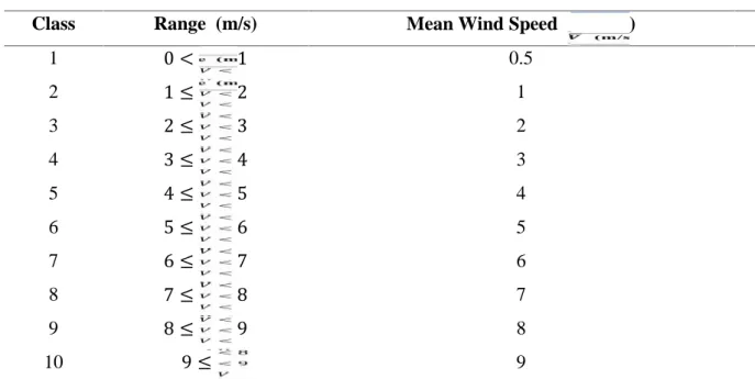
(5) D. Kidmo et al.. J Fundam Appl Sci. 2014, 6(2), 153-174. 157. Table 3. Wind Speed Classes Class. Range (m/s). 1. 0<. <1. 0.5. 2≤. <3. 2. <5. 4. <7. 6. <9. 8. 1≤. 2 3. 3≤. 4. 4≤. 5. 5≤. 6. 6≤. 7. 7≤. 8. 8≤. 9. 9≤. 10. 50. Jan. Mean Wind Speed. Feb. <2. 1. <4. 3. <6. 5. <8. 7. Mar. (m/s). 9. April. May. June. July. Aug. Sep. Oct. Nov. Dec. 45 40. Frequency (%). 35 30 25 20 15 10 5 0 1. 2. 3. 4. 5. Wind Speed classes (m/s). 6. 7. 8. Fig.1. Frequency distribution of measured daily wind speed.. 9. 10.

(6) D. Kidmo et al.. J Fundam Appl Sci. 2014, 6(2), 153-174. 158. 100 90 80 70. Frequency (%). 60 50 40 30 20. Jan. Feb. Mar. April. May. June. July. Aug. Sep. Oct. Nov. Dec. 10 0 1. 2. 3. 4. 5. Wind Speed classes (m/s). 6. 7. 8. 9. 10. Fig.2. Cumulative Frequency distribution of measured daily wind speed.. 2.3. Methods to estimate Weibull parameters The variation in wind speed are most often described by the Weibull PDF with two parameters, the dimensionless Weibull shape parameter , and the Weibull scale parameter. which have reference. values in the units of wind speed. The PDF function ( ) is given by the following [4; 10; 11; 12]: ( ) = ( ⁄ ). ( ⁄ ). Where:. . exp(−( ⁄ ) ). (1). ( ) = probability of observing wind speed = wind speed [ ⁄ ]. = Weibull scale parameter [ ⁄ ]. = Weibull shape parameter. The corresponding cumulative distribution function is given by: ( ) = 1 − exp(−( ⁄ ) ). To estimate the dimensionless shape , and the scale. (2). , parameters of the Weibull distribution. function, five methods have been computed. 2.4. Graphical method The graphical method (GM) is achieved through the cumulative distribution function. In this distribution method, the wind speed data are interpolated by a straight line, using the concept of.

(7) D. Kidmo et al.. J Fundam Appl Sci. 2014, 6(2), 153-174. 159. least squares regression [6; 11; 12]. The logarithmic transformation is the foundation of this method. By converting the equation (2) into logarithmic form, the following equation is obtained: ln[− ln 1 − ( ) ] =. ( )−. ( ). The Weibull shape and scale parameters are estimated by plotting. (3). ( ) against ln[− ln 1 −. ( ) ] in which a straight line is determined. In order to generate the line of best fit, observations. of calms should be omitted from the data. The Weibull shape parameter, , is the slope of the line and the y-intercept is the value of the term − 2.5. Maximum Likelihood method. ( ).. The Maximum Likelihood Estimation method (MLM) is a mathematical expression known as a likelihood function of the wind speed data in time series format. The MLM method is solved through numerical iterations to determine the parameters of the Weibull distribution. The shape factor k and the scale factor C are estimated by the following equations [6; 8]: =. =. ∑. Where:. ∑. )−∑. ln( ) (∑ ⁄. ln( ) ⁄. (4) (5). = number of non zero data values. = measurement interval = wind speed measured at the interval [ ⁄ ]. 2.6. Modified Maximum Likelihood method. The Modified Maximum Likelihood Estimation method (MMLM) is used only for wind speed data available in the Weibull distribution format. The MMLM method is solved through numerical iterations to determine the parameters of the Weibull distribution. The shape factor k and the scale factor c are estimated by the following equations: [6]: =. ∑. ln( ) ( ). = (1⁄ ( ) ≥ 0) ∑. (∑. ( ). ⁄. ( )) – (∑. ln( ) ( )) ⁄ ( ≥ 0). Where: ( ) = Weibull frequency with which the wind speed falls within the interval i ( ≥ 0) = Probability of wind speed. ≥0. (6) (7).

(8) D. Kidmo et al.. J Fundam Appl Sci. 2014, 6(2), 153-174. 160. 2.7. Empirical method The empirical method (EM) is considered a special case of the moment method, where the Weibull parameters k and C can be determined using average wind speed and standard deviation as follows [6]. .. =( ⁄ ). (8). = ⁄ (1 + 1⁄ ). = [(1⁄( − 1)) ∑. − ) ]. (. (9). ⁄. (10). = mean wind speed [ ⁄ ]. Where:. = standard deviation of the observed data [ ⁄ ]. 2.8. Energy pattern factor method. The energy pattern factor method (EPF) is related to the averaged data of wind speed and is defined by the following equations [6; 13]. ⁄. =. ∑. =. = 1 + 3.69⁄(. Where:. ∑. ). (11) (12). is the energy pattern factor.. The Weibull scale parameter C is determined using the following equation: =. ⁄. ∑. The standard deviation = [ (1 + 2⁄ ) −. of the observed data is determined using the equation [10]: (1 + 1⁄ )]. ⁄. (14). Where the standard gamma function is given by: ( )=∫. exp(− ). ( ) = √2. (. (15). And the gamma function can be approximated [10]: )(. ) 1+. +. −. +⋯. 2.9. Prediction Performance of the Weibull distribution model The correlation coefficient. (13). (16). and root mean square error (RMSE) analysis have been carried out. in order to determine which one of the Weibull parameter calculation methods gives a better result. These parameters can be calculated from the following equations [11], [12]: =. ∑. (. −. ). ⁄. (17).

(9) D. Kidmo et al.. =. ∑. Where:. (. ∑. ). J Fundam Appl Sci. 2014, 6(2), 153-174. (. ∑. (. ). ). is the actual data,. is the predicted data using the Weibull distribution,. 161. (18). is the. predicted data using the Weibull distribution, N is the number of observations;. 3. RESULTS For each of the five numerical methods considered in the analysis, the table 4 illustrates the monthly and yearly average of the standard deviation as well as the mean wind speed. The Weibull distribution functions for the five numerical methods, describing the wind speed frequency against the mean wind speed for the actual data on a monthly basis from 1985 to 2013, are presented in the figures 3 to 14. In these figures, the proposed methods are plotted alongside the measured wind speed frequencies. Subsequently, the tables 5 to 17 show the monthly and yearly average performance of the Weibull distribution models. The table 18 illustrates the comparison between the wind speed standard deviation predicted by the methods and the measured data. It is important to notice that the standard deviation of the measured data is the same as the standard deviation obtained using the empirical method as the same formula is used. Lastly, the Performance ranking for the proposed the Weibull distribution models are summarized in the table 19..

(10) D. Kidmo et al.. J Fundam Appl Sci. 2014, 6(2), 153-174. 162. Table 4. Mean wind speed and wind speed standard deviation Mean Wind. MLM. MMLM. GM. EM. EPF. σ. σ. σ. σ. σ. January. 1.371. 1.368. 1.452. 1.293. 1.622. 2.821. February. 1.486. 1.481. 1.594. 1.438. 1.728. 2.996. March. 1.388. 1.387. 1.463. 1.316. 1.507. 3.027. April. 1.244. 1.245. 1.298. 1.208. 1.295. 2.927. May. 1.509. 1.502. 1.625. 1.528. 1.612. 2.833. June. 1.500. 1.493. 1.609. 1.514. 1.620. 2.841. July. 1.410. 1.405. 1.518. 1.419. 1.511. 2.707. August. 1.336. 1.332. 1.440. 1.340. 1.462. 2.606. September. 1.373. 1.367. 1.486. 1.384. 1.544. 2.624. October. 1.091. 1.092. 1.140. 0.964. 1.149. 2.542. November. 1.084. 1.086. 1.145. 1.025. 1.128. 2.619. December. 1.182. 1.183. 1.245. 1.156. 1.226. 2.734. Yearly Average. 1.318. 1.316. 1.388. 1.275. 1.424. 2.773. Month. 45. Speed. 45 Measured. 40. Measured. 40. MLM. MLM. MMLM. 35. MMLM. 35. GM EPF. 25. January. 20. EM. 30. Frequency (%). Frequency (%). GM. EM. 30. EPF. 25. February. 20. 15. 15. 10. 10. 5. 5. 0. 0. 0. 1. 2. 3. 4. 5. Wind Speed (m/s). 6. 7. 8. 9. 10. 0 11. 1. 2. 3. 4. 5. Wind Speed (m/s). 6. 7. Fig.3. Monthly Weibull distribution for the five models for January and February.. 8. 9. 10. 11.

(11) D. Kidmo et al.. J Fundam Appl Sci. 2014, 6(2), 153-174. 163. 45. 45. Measured. 40. Measured. 40. MLM. MLM. 35. MMLM. 35. MMLM. GM. Frequency (%). Frequency (%). EPF. 25. March. 20. GM. 30. EM. 30. EM EPF. 25 20. 15. 15. 10. 10. 5. 5. April. 0. 0 0. 1. 2. 3. 4. 5. Wind Speed (m/s). 6. 7. 8. 9. 0 11. 10. 1. 2. 3. 4. 5. Wind Speed (m/s). 6. 7. 8. 9. 10. 11. Fig.4. Monthly Weibull distribution for the five models for March and April. 45. 45 Measured. 40 35. MMLM. MLM. 35. MMLM. GM. 30. EPF. 25 20. GM. 30. EM. Frequency (%). Frequency (%). Measured. 40. MLM. May. EM EPF. 25 20. 15. 15. 10. 10. 5. 5. 0. June. 0. 0. 1. 2. 3. 4. 5. Wind Speed (m/s). 6. 7. 8. 9. 10. 0 11. 1. 2. 3. 4. 5. Wind Speed (m/s). 6. Fig.5. Monthly Weibull distribution for the five models for May and June.. 7. 8. 9. 10. 11.

(12) D. Kidmo et al.. J Fundam Appl Sci. 2014, 6(2), 153-174. 45. 45 Measured. 40. GM. Frequency (%). EPF. 20. MMLM GM. 30. EM. 25. MLM. 35. MMLM. 30. Measured. 40. MLM. 35. Frequency (%). 164. July. EM EPF. 25 20. 15. 15. 10. 10. 5. 5. 0. August. 0. 0. 1. 2. 3. 4. 5. Wind Speed (m/s). 6. 7. 8. 9. 10. 0 11. 1. 2. 3. 4. 5. Wind Speed (m/s). 6. 7. 8. 9. 10. 11. 9. 10. 11. Fig.6. Monthly Weibull distribution for the five models for July and August. 50. 50 Measured. 45 40. MMLM. 40. GM. 35. EM. 30. Frequency (%). Frequency (%). 35. EPF. 25. September. 20. Measured. 45. MLM. GM EM. 30. EPF. 25. October. 20. 15. 15. 10. 10. 5. 5. 0. MLM MMLM. 0. 0. 1. 2. 3. 4. 5. Wind Speed (m/s). 6. 7. 8. 9. 10. 0. 11. 1. 2. 3. 4. 5. Wind Speed (m/s). 6. 7. Fig.7. Monthly Weibull distribution for the five models for September and October.. 8.

(13) D. Kidmo et al.. J Fundam Appl Sci. 2014, 6(2), 153-174. 50. 50 Measured. 45. Frequency (%). EM EPF. 25. November. 20. MMLM GM. 35. GM. 30. MLM. 40. MMLM. 35. Measured. 45. MLM. 40. EM. 30. EPF. 25. December. 20. 15. 15. 10. 10. 5. 5 0. 0 0. 1. 2. 3. 4. 5. Wind Speed (m/s). 6. 7. 8. 9. 10. 0. 11. 1. 2. 3. 4. 5. Wind Speed (m/s). 6. 7. 8. 9. 10. Fig.8. Monthly Weibull distribution for the five models for November and December.. 40 Measured. 35. MLM MMLM. 30. Frequency (%). Frequency (%). 165. GM EM. 25. EPF. 20. Yearly Average. 15 10 5 0 0. 1. 2. 3. 4. 5. Wind Speed (m/s). 6. 7. 8. Fig.9. Yearly average Weibull distribution for the five models.. 9. 10. 11. 11.

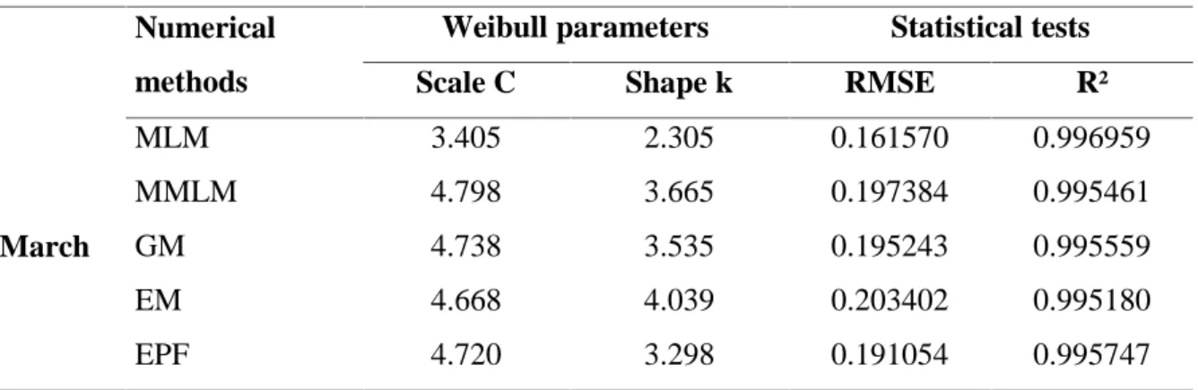
(14) D. Kidmo et al.. J Fundam Appl Sci. 2014, 6(2), 153-174. 166. Table 5. Performance of the Weibull distribution models for the month of January Numerical methods. January. Weibull parameters. Statistical tests. Scale C. Shape k. RMSE. R². MLM. 3.167. 2.155. 0.182729. 0.995503. MMLM. 4.144. 3.067. 0.206514. 0.994256. GM. 4.090. 2.932. 0.204045. 0.994392. EM. 4.014. 3.389. 0.212342. 0.993927. EPF. 4.044. 2.876. 0.202976. 0.994451. Table 6. Performance of the Weibull distribution models for the month of February Numerical methods. February. Weibull parameters. Statistical tests. Scale C. Shape k. RMSE. R². MLM. 3.373. 2.113. 0.170056. 0.996559. MMLM. 4.699. 3.138. 0.199094. 0.995284. GM. 4.665. 3.011. 0.196800. 0.995392. EM. 4.566. 3.456. 0.204614. 0.995019. EPF. 4.602. 2.935. 0.195360. 0.995459. Table 7. Performance of the Weibull distribution models for the month of March Numerical methods. March. Weibull parameters. Statistical tests. Scale C. Shape k. RMSE. R². MLM. 3.405. 2.305. 0.161570. 0.996959. MMLM. 4.798. 3.665. 0.197384. 0.995461. GM. 4.738. 3.535. 0.195243. 0.995559. EM. 4.668. 4.039. 0.203402. 0.995180. EPF. 4.720. 3.298. 0.191054. 0.995747.

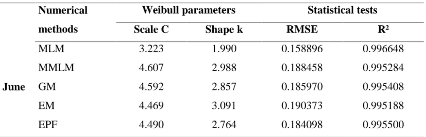
(15) D. Kidmo et al.. J Fundam Appl Sci. 2014, 6(2), 153-174. 167. Table 8. Performance of the Weibull distribution models for the month of April Numerical methods. April. Weibull parameters. Statistical tests. Scale C. Shape k. RMSE. R². MLM. 3.298. 2.518. 0.175980. 0.996133. MMLM. 4.373. 2.960. 0.190874. 0.995450. GM. 4.283. 2.846. 0.188287. 0.995573. EM. 4.239. 3.114. 0.193900. 0.995305. EPF. 4.261. 2.753. 0.186139. 0.995673. Table 9. Performance of the Weibull distribution models for the month of May Numerical methods. May. Weibull parameters. Statistical tests. Scale C. Shape k. RMSE. R². MLM. 3.215. 1.970. 0.160162. 0.996573. MMLM. 4.338. 3.026. 0.190690. 0.995141. GM. 4.261. 2.906. 0.188390. 0.995258. EM. 4.203. 3.222. 0.194398. 0.994951. EPF. 4.229. 2.812. 0.186481. 0.995354. Table 10. Performance of the Weibull distribution models for the month of June Numerical methods. June. Weibull parameters. Statistical tests. Scale C. Shape k. RMSE. R². MLM. 3.223. 1.990. 0.158896. 0.996648. MMLM. 4.607. 2.988. 0.188458. 0.995284. GM. 4.592. 2.857. 0.185970. 0.995408. EM. 4.469. 3.091. 0.190373. 0.995188. EPF. 4.490. 2.764. 0.184098. 0.995500.

(16) D. Kidmo et al.. J Fundam Appl Sci. 2014, 6(2), 153-174. 168. Table 11. Performance of the Weibull distribution models for the month of July Numerical methods. July. Weibull parameters. Statistical tests. Scale C. Shape k. RMSE. R². MLM. 3.069. 2.018. 0.166269. 0.995941. MMLM. 4.276. 2.813. 0.189624. 0.994721. GM. 4.242. 2.683. 0.187003. 0.994866. EM. 4.137. 2.878. 0.191008. 0.994643. EPF. 4.152. 2.601. 0.185264. 0.994961. Table 12. Performance of the Weibull distribution models for the month of August Numerical methods. August. Weibull parameters. Statistical tests. Scale C. Shape k. RMSE. R². MLM. 2.956. 2.054. 0.185273. 0.994554. MMLM. 3.802. 2.437. 0.197476. 0.993813. GM. 3.776. 2.297. 0.193982. 0.994030. EM. 3.650. 2.400. 0.196668. 0.993864. EPF. 3.654. 2.173. 0.190499. 0.994243. Table 13. Performance of the Weibull distribution models for the month of September Numerical methods. September. Weibull parameters. Statistical tests. Scale C. Shape k. RMSE. R². MLM. 2.978. 2.011. 0.186655. 0.994550. MMLM. 3.768. 2.310. 0.196067. 0.993987. GM. 3.762. 2.166. 0.192338. 0.994213. EM. 3.608. 2.234. 0.194201. 0.994101. EPF. 3.606. 2.016. 0.187837. 0.994481.

(17) D. Kidmo et al.. J Fundam Appl Sci. 2014, 6(2), 153-174. 169. Table 14. Performance of the Weibull distribution models for the month of October Numerical methods. October. Weibull parameters. Statistical tests. Scale C. Shape k. RMSE. R². MLM. 2.861. 2.487. 0.214529. 0.992316. MMLM. 3.660. 2.760. 0.219958. 0.991923. GM. 3.628. 2.608. 0.216685. 0.992161. EM. 3.521. 2.830. 0.221889. 0.991780. EPF. 3.534. 2.533. 0.215095. 0.992276. Table 15. Performance of the Weibull distribution models for the month of November Numerical methods. November. Weibull parameters. Statistical tests. Scale C. Shape k. RMSE. R². MLM. 2.938. 2.582. 0.210656. 0.993031. MMLM. 3.660. 2.760. 0.215223. 0.992725. GM. 3.628. 2.608. 0.211654. 0.992965. EM. 3.521. 2.830. 0.217016. 0.992604. EPF. 3.534. 2.533. 0.209758. 0.993090. Table 16. Performance of the Weibull distribution models for the month of December Numerical methods. December. Weibull parameters. Statistical tests. Scale C. Shape k. RMSE. R². MLM. 3.082. 2.471. 0.199502. 0.994282. MMLM. 4.031. 3.044. 0.213741. 0.993436. GM. 3.982. 2.904. 0.211050. 0.993600. EM. 3.902. 3.316. 0.218996. 0.993109. EPF. 3.928. 2.849. 0.209972. 0.993666.

(18) D. Kidmo et al.. J Fundam Appl Sci. 2014, 6(2), 153-174. 170. Table 17. Performance of the Weibull distribution models for the yearly average Numerical methods. Yearly Average. Weibull parameters. Statistical tests. Scale C. Shape k. RMSE. R². MLM. 3.130. 2.223. 0.178758. 0.995540. MMLM. 3.994. 3.174. 0.203103. 0.994242. GM. 3.960. 3.022. 0.200267. 0.994402. EM. 3.867. 3.548. 0.209996. 0.993844. EPF. 3.900. 2.981. 0.199513. 0.994444. Table 18. Comparison between the wind speed standard deviation predicted by the methods and the measured data Months. MLM. MMLM. GM. EM. EPF. January. -6.07%. -5.82%. -12.31%. 0.00%. -25.49%. February. -3.35%. -3.03%. -10.86%. 0.00%. -20.18%. March. -5.47%. -5.37%. -11.18%. 0.00%. -14.51%. April. -2.97%. -3.06%. -7.42%. 0.00%. -7.21%. May. 1.19%. 1.66%. -6.41%. 0.00%. -5.51%. June. 0.94%. 1.39%. -6.28%. 0.00%. -6.96%. July. 0.63%. 1.02%. -6.95%. 0.00%. -6.48%. August. 0.27%. 0.60%. -7.49%. 0.00%. -9.14%. September. 0.84%. 1.23%. -7.33%. 0.00%. -11.57%. October. -13.12%. -13.26%. -18.21%. 0.00%. -19.16%. November. -5.78%. -5.97%. -11.69%. 0.00%. -10.08%. December. -2.26%. -2.34%. -7.70%. 0.00%. -6.06%. Yearly Average. -3.33%. -3.17%. -8.86%. 0.00%. -11.67%.

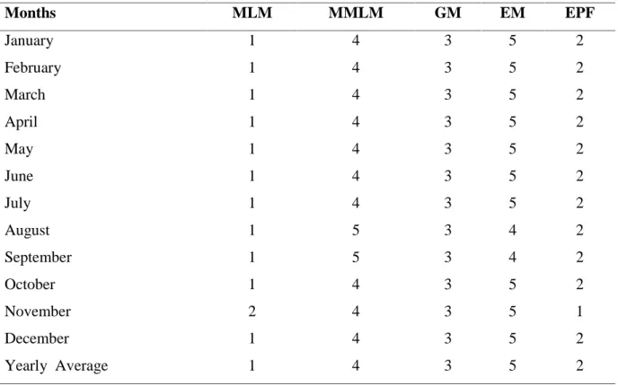
(19) D. Kidmo et al.. J Fundam Appl Sci. 2014, 6(2), 153-174. 171. Table 19. Performance ranking for of the five Weibull distribution models Months. MLM. MMLM. GM. EM. EPF. January. 1. 4. 3. 5. 2. February. 1. 4. 3. 5. 2. March. 1. 4. 3. 5. 2. April. 1. 4. 3. 5. 2. May. 1. 4. 3. 5. 2. June. 1. 4. 3. 5. 2. July. 1. 4. 3. 5. 2. August. 1. 5. 3. 4. 2. September. 1. 5. 3. 4. 2. October. 1. 4. 3. 5. 2. November. 2. 4. 3. 5. 1. December. 1. 4. 3. 5. 2. Yearly Average. 1. 4. 3. 5. 2. 4. DISCUSSIONS 4.1. Performance of the Weibull distribution models As mentioned earlier, there is no doubt that the Weibull PDF with two parameters, the dimensionless shape parameter k, and the scale parameter C, is a good quality probabilistic model for wind speed in the district of Maroua. Therefore, the proposed five methods are effective in evaluating the parameters of the Weibull distribution for the available data. Obviously, the more suitable Weibull estimation method shall provide accurate and efficient evaluation of wind energy potential. The performance of the proposed five models were carried out based on the correlation coefficient. and the root mean square error (RMSE) analysis in order to determine which one of. the Weibull parameter calculation methods gives a better result. The best parameters estimation shall contain the lowest value of RMSE and the highest value of R². As a result, the performance rankings for the five Weibull distribution models are provided in the Table 19. Overall, the maximum likelihood method is the most accurate model followed by the energy pattern factor method and the graphical method. The least precise models are the empirical method followed by.

(20) D. Kidmo et al.. J Fundam Appl Sci. 2014, 6(2), 153-174. 172. the modified maximum likelihood method. Furthermore, it is observed that the values of RMSE, and R², have magnitudes very close to each other for all the numerical methods used for the collected data. The table 18 illustrates the comparison between the wind speed standard deviation predicted by the five models and the measured data. It can be noticed that the maximum likelihood method has a smaller relative error of -3.33% on average compared to -11.67% for the energy Pattern Factor method. The standard deviation formula for the measured data is the same as the standard deviation formula for the empirical method, hence the relative error of 0.00% for the empirical method. 4.2. Weibull distribution model parameters. and. The Weibull shape k parameter indicates the breadth of a distribution of wind speeds. Lower k values mean that winds tend to vary over a large range of speeds while higher k values correspond to wind speeds staying within a narrow range. When considering the maximum likelihood method as the most accurate Weibull distribution model, it’s observed that Weibull k values range from 1.970 in the month of May to 2.582 in the month of November. Typical Weibull k value for most wind conditions ranges from 1.500 to 3.000 [14]. On the other hand, the Weibull scale C parameter shows how “windy” a location is or, in other words, how high the annual mean speed is. When considering the maximum likelihood method as the most accurate Weibull distribution model, it’s as well observed that Weibull C values vary from 2.861 of October to 3.405 of March. These two Weibull parameters determine the wind speed for optimum performance of a WECS as well as the speed range over which it’s expected to operate.. 5. CONCLUSION Based on the data collected in the district of Maroua, the aim of this work was to provide an insightful analysis to engineers when selecting a method that gives more accurate estimation for the Weibull parameters in order to reduce uncertainties related to the wind energy output calculation from any WECS. The following main conclusions can be drawn from the present study: 1. Monthly and average yearly performances of the Weibull distribution for the five proposed models were carried out based on the correlation coefficient R and root mean square error (RMSE);.

(21) D. Kidmo et al.. J Fundam Appl Sci. 2014, 6(2), 153-174. 173. 2. The proposed five methods are effective in evaluating the parameters of the Weibull distribution for the available data since the values of RMSE, and R² have magnitudes very close to each other for the collected data in the district of Maroua, Cameroon; 3. The performance comparison of the proposed methods established that the most accurate models are the maximum likelihood method followed by the energy pattern factor method and the graphical method. The least precise models are the empirical method followed by the modified maximum likelihood method. 4. The comparison between the wind speed standard deviation predicted by the models and the measured data showed a smaller relative error using the maximum likelihood method than using the energy pattern factor method or the graphical method, the most accurate models; 5. The results therefore, strongly suggest, based on the collected data in the district of Maroua, that the maximum likelihood method is more reliable in estimating Weibull shape and scale parameters. Consequently, the yearly average for the Weibull k value is 2.222 while the yearly average for the Weibull C value is 3.130.. 6. REFERENCES [1] Abdeen Mustafa Omer. Wind mechanical engineering: energy for water pumping in rural areas in sudan. Technical Proceedings of the 2011 Clean Technology Conference and Trade Show, Chapter 1: Renewable Energy Technologies, pp. 21-24. [2] C.G. Justus, W.R. Hargraves, Amir mikail and denise grabber. Methods for estimating speed frequency distributions, Journal of applied meteorology, volume 17, Nov. 1977, pp. 350-353. [3] C.G. Justus, W.R. Hargraves, and Ali Yalcin. Nationwide assessment of potential output from wind-powered generators, Journal of applied meteorology, vol. 15, N° 7 July 1976, pp. 673678. [4] E.H. lysen. Introduction to wind energy, Consultancy Services Wind Energy Developing Countries, CWO 82 May 1, 1983 (2nd edition), pp. 36-37. [5] Mukund R. Patel. Wind and Solar Power Systems, U.S. Merchant Marine Academy Kings Point, New York, 1999 by CRC Press LLC, pp. 59-61. [6] P. A. Costa Rocha, R. Coelho de Sousa, C. Freitas de Andrade, M. Vieira da Silva. Comparison of seven numerical methods for determining Weibull parameters for wind energy generation in the northeast region of Brazil, Applied Energy 89 (2012) pp. 395–400..

(22) D. Kidmo et al.. J Fundam Appl Sci. 2014, 6(2), 153-174. 174. [7] K. Conradsen and L.B. Nielsen. Review of Weibull statistics for estimation of wind speed distributions, American meteorological society, Aug. 1984 vol. 23, pp. 1173-1183. [8] D. Deligiorgi, D. Kolokotsa, T. Papakostas, E. Mantou. Analysis of the Wind Field at the Broader Area of Chania, Crete, Proc. of the 3rd IASME/WSEAS Int. Conf. on Energy, Environment, Ecosystems and Sustainable Development, Agios Nikolaos, Greece, July 24-26, 2007, pp. 270-275. [9] Salahaddin A. Ahmed. Comparative study of four methods for estimating Weibull parameters for Halabja, Iraq, International Journal of Physical Sciences Vol. 8(5), pp. 186-192, 9 February, 2013, pp 186-192. [10] Manwell, J.F., McGowan, J.G., and & Rogers, A.L. Wind energy explained: Theory, design and application, John Wiley and Sons Ltd. 2002, pp 57-60. [11] Pavia, E.G. & O’Brian, J.J. Weibull statistics of wind speed over the ocean, Journal of Climate and applied meteorology, American meteorological society, October 1986, vol.25, pp. 13241332. [12] Paritosh Bhattacharya. A study on Weibull distribution for estimating the parameters, Journal of Applied Quantitative methods, summer 2010, Vol 5 N°2, pp. 234-214. [13] Odo, F.C. & Akubue, G.U. Comparative Assessment of Three Models for Estimating Weibull Parameters for Wind Energy Applications in a Nigerian Location, International Journal of energy science, IJES, 2012, Vol.2 N°1 pp.22-25. [14] Waewsak, J., Chancham, C., Landry, M., & Gagnon, Y. An Analysis of Wind Speed Distribution at Thasala, Nakhon Si Thammarat, Thailand, Journal of Sustainable Energy & Environment 2 (2011) pp 51-55.. How to cite this article: Kidmo Kaoga D. Raidandi D. Yamigno Doka S. Djongyang N. Performance analysis of twoparameter weibull distribution methods for wind energy applications in the district of Maroua, Cameroon. J Fundam Appl Sci. 2014, 6(2), 153-174..

(23)