HAL Id: hal-01387299
https://hal.inria.fr/hal-01387299
Submitted on 25 Oct 2016
HAL is a multi-disciplinary open access
archive for the deposit and dissemination of
sci-entific research documents, whether they are
pub-lished or not. The documents may come from
teaching and research institutions in France or
L’archive ouverte pluridisciplinaire HAL, est
destinée au dépôt et à la diffusion de documents
scientifiques de niveau recherche, publiés ou non,
émanant des établissements d’enseignement et de
recherche français ou étrangers, des laboratoires
Command-based importance sampling for statistical
model checking
Cyrille Jegourel, Axel Legay, Sean Sedwards
To cite this version:
Cyrille Jegourel, Axel Legay, Sean Sedwards.
Command-based importance sampling for
sta-tistical model checking.
Theoretical Computer Science, Elsevier, 2016, 649, pp.1 - 24.
�10.1016/j.tcs.2016.08.009�. �hal-01387299�
Command-based Importance Sampling for Statistical
Model Checking
Cyrille Jegourel, Axel Legay and Sean Sedwards
INRIA Rennes – Bretagne Atlantique
Abstract
Statistical model checking avoids the exponential growth of states of numerical model checking, but rare properties are costly to verify. Importance sampling can reduce the cost if good importance sampling distributions can be found efficiently.
Our approach uses a tractable cross-entropy minimisation algorithm to find an optimal parametrised importance sampling distribution. In contrast to pre-vious work, our algorithm uses a naturally defined low dimensional vector to specify the distribution, thus avoiding an explicit representation of a transition matrix. Our parametrisation leads to a unique optimum and is shown to pro-duce many orders of magnitude improvement in efficiency on various models. In this work we link the existence of optimal importance sampling distributions to logical properties and show how our parametrisation affects this link. We also motivate and present simple algorithms to create the initial distribution neces-sary for cross-entropy minimisation. Finally, we discuss the open challenge of defining error bounds with importance sampling and describe how our optimal parametrised distributions may be used to infer qualitative confidence.
1. Introduction
The most common method to ensure the correctness of a system is by test-ing it with a number of test cases havtest-ing predicted outcomes that can highlight specific problems. Such testing techniques remain the default in industrial con-texts and have also been incorporated into sophisticated tools [1]. Despite this, testing is limited by the need to hypothesise scenarios that may cause failure and the fact that a reasonable set of test cases is unlikely to cover all possible eventualities. Errors and modes of failure in complex systems may remain un-detected and quantifying the likelihood of failure using a series of test cases is difficult.
Static analysis has been successful in debugging very large systems [2], but its ability to analyse dynamical properties is limited by its level of abstraction. In contrast, model checking is a fine-grained exhaustive technique that verifies whether a system satisfies a dynamical temporal logic property under all possible scenarios. In recognition of the existence of nondeterministic and probabilistic
systems, and the fact that a Boolean answer is not always useful, numerical model checking quantifies the probability that a system satisfies a property. Numerical model checking offers precise and accurate analysis by exhaustively exploring the state space of probabilistic systems. The result of this technique is the notionally exact probability (i.e., within the limits of numerical precision and convergence stability) that a system will satisfy a property of interest, however the exponential growth of the state space limits its applicability. The typical state limit of exhaustive approaches usually represents an insignificant fraction of the state space of “real” systems. Such systems may have tens of orders of magnitude more states than the number of protons in the universe (≈ 1080).
Symbolic model checking using efficient data structures can make certain very large models tractable [3]. It may also be possible to construct simpler but behaviourally equivalent abstractions using various symmetry reduction tech-niques, such as partial order reduction, bisimulation and lumping [4]. Composi-tional approaches may also help. In particular, components of a system may be specified in such a way that each is tractable to analysis, while their properties guarantee that certain faults are impossible. Despite these techniques, however, the size, unpredictability and heterogeneity of real systems [5] often make nu-merical techniques infeasible. Moreover, even if a system has been specified not to misbehave, it is nevertheless necessary to check that it meets its specification. While the ‘state explosion problem’ [6] is unlikely to ever be entirely solved for all systems, simulation-based approaches are becoming increasingly tractable due to the availability of high performance parallel hardware and algorithms. In particular, statistical model checking (SMC) combines the simplicity of testing with the formality of numerical model checking. The core idea of SMC is to create multiple independent execution traces of the system and individually verify whether they satisfy some formally specified property. The proportion of satisfying traces is an estimate of the probability that the system satisfies the property. By thus modelling the executions of a system as a Bernoulli random variable, the absolute error of the estimate can be bounded using, for example, a confidence interval [7, Chap. 1] or a Chernoff bound [8, 9, 10]. It is also possible to use efficient techniques, such as Bayesian inference [11] and hypothesis testing [12, 13], to decide with specified statistical confidence whether the probability of a property is above or below a given threshold.
Knowing a result with less than 100% confidence is often sufficient in real applications, since the confidence bounds may be made arbitrarily tight. More-over, a swiftly achieved approximation may prevent a lot of wasted time during model design. For many complex systems, SMC offers the only feasible means of quantifying performance. Evidence of this is that SMC has been used to find bugs in large, heterogeneous aircraft systems [5]. Dedicated SMC platforms in-clude APMC [14], YMER [15], VESTA [16], PLASMA [17] and COSMOS [18]. Well-established numerical model checkers, such as PRISM [19] and UPPAAL [20], are now also including SMC engines. Indeed, since SMC may be applied to any discrete event trace obtained by stochastic simulation, [21] describes a mod-ular library of SMC algorithms that may be used to construct domain-specific SMC tools.
SMC relies on multiple independent simulations, so it may be efficiently divided on parallel computer architectures, such as grids, clusters, clouds and general purpose computing on graphics processors (GPGPU). Despite this, rare properties require a challenging number of simulations. Standard error bounding strategies for SMC consider absolute error. As the probability of a property decreases, however, it is more useful to consider an error bound that is relative to the probability. The number of simulations required to bound the relative error, defined as the standard deviation of the estimate divided by its expectation, is inversely proportional to rarity. Hence, while SMC may make a verification task feasible, it may nevertheless be computationally intense. To address this problem, in this work we apply the variance reduction technique of importance
sampling to statistical model checking.
Importance sampling works by simulating a system under a weighted (im-portance sampling) distribution that makes a property more likely to be seen. It then compensates the results by the weights, to estimate the probability under the original distribution. The concept arose from work on the ‘Monte Carlo method’ [22] in the 1940s and was originally used to quantify the performance of materials and solve otherwise intractable analytical problems with limited computer power (see, e.g., [23]).
For importance sampling to be effective it is necessary to define a “good” importance sampling distribution: (i ) the property of interest must be seen frequently in simulations and (ii ) the distribution of the simulation traces that satisfy the property in the importance sampling distribution must be as close as possible to the normalised distribution of the same traces in the original distribution. Failure to consider both (i ) and (ii ) can result in gross errors and overestimates of confidence. Moreover, the process of finding a good importance sampling distribution must itself be efficient and, in particular, should not rely on iterating over all the states or transitions of the system. The algorithms we present in this work address all these issues.
The term ‘rare event’ is ubiquitous in the literature. Here we specifically consider rare properties of paths, defined in bounded temporal logic (bounded by time or number of steps). This extends the common notion of rarity from states to paths. States are rare if the probability of reaching them from the initial state is small. Paths are rare if the probability of executing their se-quence of states is unlikely–whether or not the states themselves are rare. Rare properties are therefore more general than rare states, however the distinction does not significantly alter the mathematical derivation of our algorithms. It can nevertheless affect the existence of the so-called “zero variance” optimal importance sampling distribution as a simple re-parametrisation of the states and transitions of the original system. We explore this important subject in Section 7.
1.1. Contribution
This work extends [24], describing the additional techniques necessary to apply our importance sampling framework for statistical model checking of rare events. We describe simple algorithms to initiate the cross-entropy minimisation
process by finding at least a few traces that satisfy the property. We believe this subject has been glossed over in previous work. Simple heuristics, such as unifying the probabilities of transitions from a given state, may fail if rarity is not related to low probability transitions. We also describe and illustrate some of the key phenomena relating to parametrised importance sampling and clarify some recent misconceptions about confidence.
To apply SMC to discrete space Markov models with rare properties, our approach is based on a simply-implemented cross-entropy minimisation algo-rithm that finds an optimal set of parameters to characterise an importance sampling distribution. We have previously shown that there is a unique opti-mum and that our algorithm converges [24]. Our parametrisation is at the level of guarded commands [25] and arises naturally from standard syntactic descrip-tions of models. It is thus a very tractable low dimensional vector in comparison to the state space of the model. As such, the family of distributions induced by the parametrisation is unlikely to contain the zero variance distribution, but this is not necessary for practical applications. In practice, it is sufficient to reduce the variance without over-emphasising any particular part of the trace space. We contend that a parametrisation at the level of a low level syntax, as in our case, is well placed to achieve this efficiently. Such a syntactical descrip-tion of a model necessarily defines the symmetries evident in the distribudescrip-tion of behaviour and typically contains specific elements relevant to the property of interest.
While there will always exist pathological systems and models that are in-tractable to our approach, we are able to demonstrate very substantial reduc-tions in variance on a number of models with very few parameters. To illustrate the theoretical benefits, though not necessarily practical benefits, we also show how increasing the number of parameters of a model allows the parametrised importance sampling distribution to better approximate the zero variance dis-tribution.
1.2. Related work
Importance sampling was invented as a means to accelerate simulations of rare events [23]. Since then it has become a standard technique to allow the behaviour of a system with an “inconvenient” distribution to be simulated by a more convenient one. Cross-entropy (also known as Kullback-Leibler divergence [26]) is a standard information-theoretic measure of directed distance between distributions. The cross-entropy method [27, 28] is an algorithmic framework that facilitates the convergence of an arbitrarily parametrised distribution to an optimal distribution, without an explicit (closed form) representation of the optimal distribution. Given the general applicability of these techniques, in what follows we highlight only those recent contributions that are of specific relevance to the present work.
As a precursor to SMC, earlier work considered ‘highly reliable systems’ comprising components that fail probabilistically and are then repaired [29, 30, 31]. Since many critical systems need to be highly reliable, failure is often a rare event of critical importance. A challenge arises because real systems tend to
have a size and complexity that is intractable to exhaustive analysis. A focus of research in this field is therefore finding good parametrised importance sampling distributions that do not require analysis at the level of individual transition probabilities.
In [29] the author defines two structural properties of Markovian systems that allow good importance sampling distributions to be created by ‘simple fail-ure biasing’. If (i ) a repair is possible in any state and (ii ) the failfail-ure rates are balanced (i.e., bounded), then an importance sampling estimator that merely biases the failure rate can have a bounded relative error. If only (i ) holds, the same work proposes a ‘balanced failure biasing’ algorithm that finds a simi-larly good importance sampling distribution. If (i ) does not hold, such biasing schemes may fail due to the existence of high probability cycles with ‘group repair’ (simultaneous repair of multiple failed components). To address this problem, in [32, 33] the authors propose increasingly complex biasing schemes that make use of other structural properties.
In [31] the author defines an algorithm to construct optimal importance sampling distributions for repair models, using the cross-entropy method [27]. By parametrising a system at the level of individual transition probabilities (effectively the lowest possible level), the algorithm will converge to the perfect ‘zero variance’ importance sampling distribution (defined in Section 3) when it exists (see Section 7). Hence, [31] addresses the problem of systems containing group repair, but at the prohibitive cost of iterating over every transition. Since numerical algorithms have similar complexity, but avoid the cost of simulation and give results with near certainty, [31] does not provide a practical solution for SMC.
In [34] the authors construct an importance sampling distribution for ‘highly dependable systems’, based on dominant paths to failure. The authors frame their results in the context of (statistical) model checking, but focus on a stan-dard reliability model and do not consider the specific problems that logical properties incur. While the results may not be generalisable, by constructing distributions based on an analysis of bounded paths, the work nevertheless hints at future directions of research applying rare event techniques to SMC.
In [35] the authors present a specific application of the cross-entropy method to a simple continuous time failure model. The system comprises independent components that fail at times that are exponentially distributed. By consid-ering the first simultaneous failure of all components, the authors are able to use a standard closed form solution to find an importance sampling distribution that increases the occurrence of this rare event. Although the notions of tem-poral logic and SMC are introduced, they effectively play no part because the technique is not generalisable to other properties or systems.
In [36] the authors attempt to address the important challenge of bounding the error of estimates when using importance sampling with SMC (we discuss this open challenge in Section 8). The work contains some interesting ideas, but does not yet provide practical solutions. The basic notion is to perform numerical analysis on a reduced (abstracted) model of a system, in order to infer on the fly an importance sampling distribution that guarantees statistical
confidence. The authors assume the existence of a suitable property-specific abstraction function that maps states in the full model to states in the abstracted model, such that all abstracted traces that satisfy the property have probability greater than or equal to the traces they abstract. No algorithmic means of generating such a function is provided and we believe this is generally non-trivial. The ‘coupling’ mentioned in the title is included as a way to verify that an existing function is correct.
Importance splitting is another variance reduction technique developed in the 1940s [23]. Rather than modify the dynamics of the system, as in the case of importance sampling, the technique relies on properties that may be decomposed into a sequence of dependent ‘levels’. The overall probability is thus decomposed into the product of probabilities of going from one level to the next. Since these probabilities are necessarily larger than the overall probability, their estimation is generally easier. In [37] the authors define how importance splitting may be used to verify rare properties in the context of statistical model checking, defining how properties specified in temporal logic may be decomposed into levels. Importance sampling and splitting are not mutually exclusive, hence future work may combine them in the context of SMC.
1.3. Structure of the Article
Section 2 describes notation we will use in the sequel, while Section 3 intro-duces the basic notions of Monte Carlo integration and importance sampling. Section 4 introduces the cross-entropy minimisation framework. Our command-based cross-entropy minimisation approach is fully described in Section 5, with the results of applying it to some case studies given in Section 6. In Section 7 we consider the conditions under which optimal importance sampling distribu-tions exist as parametrisadistribu-tions of the original system. In Section 8 we discuss the challenges of specifying the confidence of importance sampling estimates. Section 9 concludes the paper.
2. Preliminaries
We consider systems described by discrete and continuous time Markov chains that may be infinite. We assume the models are specified by a set of stochastic guarded commands (‘commands’ for short) acting in parallel. Each command has the form (guard, rate, action). The guard enables the command and is a predicate over the state variables of the model. The rate is a function from the state variables toR>0, defining the rate of an exponential distribution.
The action is an update function that modifies the state variables. In general, each command defines a set of semantically linked transitions in the resulting Markov chain. Models are thus described in a relatively compact and conve-nient way. The widely adopted PRISM language1 is an example of a modelling
language based on stochastic guarded commands.
The semantics of a stochastic guarded command is a Markov jump process. The semantics of a parallel composition of commands is a system of concurrent Markov jump processes. Sample execution traces can be generated by discrete-event simulation (e.g., [38]). In any state, zero or more commands may be enabled. If no commands are enabled the system is in a halting state. In all other cases the enabled commands “compete” to execute their actions: sample times are drawn from the exponential distributions defined by their rates and the shortest time “wins”.
Execution traces (equivalently paths) are thus sequences of the form ω =
s0 t0 → s1 t1 → s2 t2
→ ..., where each si ∈ S is a state of the model and ti ∈ R>0
is the time spent in the state si (the delay time) before moving to the state
si+1. In the case of discrete time, ti≡ 1, ∀i. When we are not interested by the
times of jump epochs, we denote a trace ω = s0s1.... The length of trace ω is
the number of transitions it contains and is denoted|ω|. We denote by ω≥kthe suffix of ω starting at sk, i.e., sksk+1· · · .
2.1. Statistical Model Checking
The process of statistical model checking estimates the probability that a system satisfies a property by the proportion of simulation traces in a random sample that individually satisfy it. To achieve this, the statistical model checker constructs an automaton to accept only traces satisfying a property specified using time bounded temporal logic. Given a randomly generated trace ω, the automaton outputs a 1 if ω is accepted and 0 otherwise. Statistical model check-ing can thus be seen as the estimation of the success parameter of a Bernoulli random variable with support {0, 1}. By using this abstraction, SMC is also able to test hypotheses about the parameter and inherits theory that allows the statistical confidence of results to be calculated.
The following abstract syntax is typical of a bounded linear temporal logic used in SMC:
φ = α| φ ∨ φ | φ ∧ φ | ¬φ | Xφ | Ftφ| Gtφ| φUtφ (1) Symbol α denotes an atomic proposition that may be true or false in any state
s ∈ S. Operators ∨, ∧ and ¬ are the standard Boolean connectives. Ft, Gt
and Utare temporal operators that apply to time interval [0, t], where t∈ R >0
may denote steps or real time and the interval is relative to the interval of any enclosing operator. We refer to this informally as a “relative interval”. To simplify the following notation, it is assumed that if a property requires the next state to be satisfied and no next state exists, the property is not satisfied. Thus, given a property φ with syntax (1), the semantics of the satisfaction relation
ω|= φ ≡ ω≥0|= φ is inductively defined as follows: • ω≥k|= α ⇐⇒ α evaluates to true in state sk
• ω≥k|= φ1∨ φ2 ⇐⇒ ω≥k|= φ1∨ ω≥k|= φ2 • ω≥k|= φ1∧ φ2 ⇐⇒ ω≥k|= φ1∧ ω≥k|= φ2
• ω≥k|= ¬φ ⇐⇒ ω≥k̸|= φ
• ω≥k|= Xφ ⇐⇒ ω≥k+1|= φ
• ω≥k|= Ftφ ⇐⇒ ∃i ≥ k ∈ N :∑l∈{k,...,i}tl≤ t ∧ ω≥i|= φ
• ω≥k |= Gtφ ⇐⇒ ∃i ≥ k ∈ N : ∑l∈{k,...,i}tl ≤ t ∧ ∑ l∈{k,...,i+1}tl > t∧ ∀l ∈ {k, . . . , i} : ω≥l|= φ • ω≥k |= φ1Utφ2 ⇐⇒ ∃i ≥ k ∈ N : ∑ l∈{k,...,i}tl ≤ t ∧ ω≥i|= φ2∧ (i = k∨ ∀l ∈ {k, . . . , i − 1} : ω≥l|= φ1)
Ft, Gtand Utare related in the following way: Gt=¬(Ft¬φ), Ftφ = trueUtφ,
hence Gtφ =¬(trueUt¬φ). Informally: Xφ means that φ will be true in the
next state; Ftφ means that φ will be true at least once in the relative interval
[0, t]; Gtφ means that φ will always be true in the relative interval [0, t]; ψUtφ
means that in the relative interval [0, t], φ will eventually be true and ψ will be true until it is.
3. Monte Carlo Integration and Importance Sampling
Statistical model checking is based on the concept of Monte Carlo integra-tion [39, Ch. 3]. Given a random variable X, with sample space ω ∈ Ω and distribution f , the expectation of an integrable function z(X) can be expressed as
Ef[z(X)] =
ˆ
Ω
z(ω) df (ω). (2)
To estimate Ef[z(X)], Monte Carlo integration works by drawing N samples
ωi, i∈ {1, . . . , N}, at random according to distribution f and calculating
Ef[z(X)]≈ 1 N N ∑ i=1 z(ωi). (3)
With increasing N , the right hand side of (3) is guaranteed to converge to the left hand side by the law of large numbers. In the context of SMC, Ω is a probability space of paths, f is the probability measure over Ω and z represents the output of the model checking automaton described in Section 2.1. Later, in the specific context of SMC, we denote this particular function z by1(ω |= φ), to emphasise its characteristics.
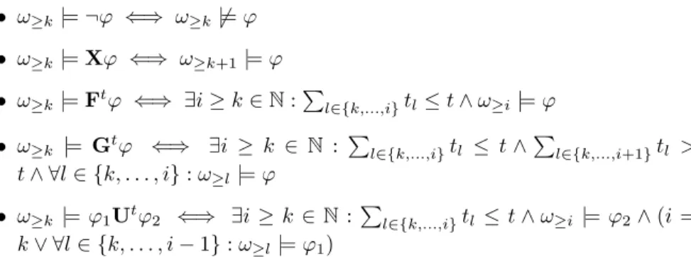
Figure 1a illustrates how (3) works. The outer square denotes the space of all traces Ω, the leaf shape denotes the set of traces that satisfy φ. The red dots are uniformly sampled at random from Ω, such that the fraction of samples falling within the leaf is an approximation of the probability that the system will satisfy φ. Figure 1b illustrates the problem when a property is rare. Fewer samples fall within the leaf and, moreover, the coverage of the leaf is apparently less uniform than in Fig. 1a. Unbiased convergence is still guaranteed with increasing N , but the variance of the estimate is higher.
Equation (3) can thus be used to estimate the probability that a system will satisfy a property φ, where γ is defined by
γ =
ˆ
Ω
z(ω) df (ω) (4)
and the standard “crude” Monte Carlo estimator of γ can be written
˜ γ = 1 NMC N∑MC i=1 z(ωi). (5)
NMC denotes the number of simulations used by the standard Monte Carlo
estimator and ωi is sampled according to f , denoted ωi ∼ f. Note that z(ωi)
is effectively the realisation of a Bernoulli random variable with parameter γ. Hence Var(˜γ) = γ(1− γ)/NMC and for γ→ 0, Var(˜γ) ≈ γ/NMC.
Let f be absolutely continuous with respect to another probability measure
f′ over Ω, then (4) can be written
γ = ˆ Ω z(ω)df (ω) df′(ω)df ′(ω). (6)
L = df /df′ is the likelihood ratio function, so
γ =
ˆ
Ω
L(ω)z(ω) df′(ω). (7)
We can thus estimate γ by simulating under f′ and compensating by L:
˜ γ = 1 NIS NIS ∑ i=1 L(ωi)z(ωi) (8)
Here ωi∼ f′and NISdenotes the number of simulations used by the importance
sampling estimator. The goal of importance sampling is to reduce the variance of the rare event and so achieve a narrower confidence interval than the Monte Carlo estimator, resulting in NIS≪ NMC. In general, the importance sampling
distribution f′is chosen to produce the rare property more frequently. Figure 1c illustrates the basic notion of importance sampling. The sampling distribution is weighted in such a way that most of the samples fall within the leaf. The fraction of samples falling within the leaf is no longer an approximation of the probability we seek, but knowing the values of the weights it is possible to compensate and calculate an unbiased estimate.
The optimal importance sampling distribution, denoted f∗ and defined as f conditioned on the rare event, produces only traces satisfying the rare property. Formally, we define f∗by
df∗= z df
γ . (9)
Figure 1d illustrates the notion of the optimal importance sampling distribution. All the samples fall within the leaf and the coverage is uniform. This leads to
(a) (b) (c)
(d) (e) (f)
Figure 1: Monte Carlo integration.
the term ‘zero variance estimator’, since under f∗, traces for which z = 0 have zero probability of being seen and L = γ whenever z = 1. Note, however, that in general the optimal importance sampling distribution f∗does not itself have zero variance.
In practice, it is usually only possible to observe the percentage of success-ful simulations and not possible to judge how uniformly the distribution covers the target area. Moreover, the percentage of success does not necessarily in-dicate the quality of the importance sampling distribution. For example, the distribution illustrated in Fig. 1e produces 100% success but is focused on only a small percentage of the target area. This distribution will have low sample variance, giving a false impression of high confidence, but will produce a severe underestimate of the true probability.
Figure 1f illustrates the notion of a minimum cross-entropy parametrised distribution. The distribution is more focused than Fig. 1c, but not pathologi-cally so, like Fig. 1e. It does not perfectly cover the leaf, like the theoretipathologi-cally optimal distribution of Fig. 1d, because the optimal distribution is not a mem-ber of the family generated by its particular parametrisation. Intuitively, the minimum cross-entropy distribution is one which optimally balances focus and coverage, given the parametrisation.
3.1. Importance Sampling for Parametrised Systems
Importance sampling schemes have been described as falling into two broad categories: state dependent tilting and state independent tilting [40]. State
de-pendent tilting refers to importance sampling distributions that individually weight (‘tilt’) every transition probability in the system. State independent tilting refers to importance sampling distributions that change classes of transi-tion probabilities, independent of state. State dependent tilting offers greatest precision, but is infeasible in a large model unless it can be done on the fly by a function that exploits the model’s symmetries. Such symmetries do not always exist in real systems. State independent tilting is more tractable but may not produce good importance sampling distributions. Our approach may be seen as
parametrised tilting, that potentially affects all transitions differently, but does
so according to a set of parameters.
In the context of SMC, the distribution f introduced in Section 3 usually arises from the specifications of a model described in some relatively high level language. Such models do not, in general, explicitly specify the probabilities of individual transitions, but do so implicitly by parametrised functions over the states. We therefore consider a class of models that can be described by guarded commands [25] extended with stochastic rates. Our parametrisation is a vector of strictly positive values λ∈ Rn>0 that tilt (multiply) the stochastic rates and thus maintain the absolutely continuous property between distributions. Note that this class includes both discrete and continuous time Markov chains and that in the latter case our mathematical treatment works with the embedded discrete time process.
In what follows we are therefore interested in parametrised distributions and write f (·, λ), where λ = {λ1, . . . , λn} is a vector of parameters, and distinguish
different probability measures by their parameters. In particular, we denote by µ the original vector of parameters of the model and f (·, µ) is therefore the original measure. We can thus rewrite (7) as
γ =
ˆ
Ω
L(ω)z(ω) df (ω, λ), (10)
where L(ω) = df (ω, µ)/df (ω, λ). We can also rewrite (9) as df∗ =z df (·, µ)
γ (11)
and write f (·, λ∗) for the optimal parametrised measure. We define the optimal parametrised measure as that which minimises the cross-entropy [26] between
f (·, λ) and f∗ for a given parametrisation and note that, in general, f∗ ̸=
f (·, λ∗).
4. The Cross-Entropy Method
Cross-entropy [26] (alternatively relative entropy or Kullback-Leibler diver-gence) has been shown to be a uniquely correct directed measure of distance between distributions [41]. With regard to the present context, it has also been shown to be useful in finding optimum distributions for importance sampling [28, 40, 31].
Given two probability measures f and f′over the same probability space Ω, the cross-entropy from f to f′ is given by
CE(f, f′) = ˆ Ω log df (ω) df′(ω)df (ω) (12) = ˆ Ω log df (ω) df (ω)− ˆ Ω log df′(ω) df (ω) = H(f )− ˆ Ω log df′(ω) df (ω), (13)
where H(f ) is the entropy of f . To find λ∗ we minimise CE(zf (γ·,µ), f (·, λ)),
noting that H(f (·, µ)) is independent of λ:
λ∗= arg max
λ
ˆ
Ω
z(ω) log df (ω, λ) df (ω, µ) (14) Estimating λ∗directly using (14) is difficult, so we re-write it using importance sampling measure f (·, λ′) and likelihood ratio L(ω) = df (ω, µ)/df (ω, λ′):
λ∗= arg max
λ
ˆ
Ω
z(ω)L(ω) log df (ω, λ) df (ω, λ′) (15) Using (15) we can construct an unbiased importance sampling estimator of λ∗ and use it as the basis of an iterative process to obtain successively better estimates: ˜ λ∗= λ(j+1)= arg max λ N ∑ i=1 z(ω(j)i )L(j)(ω(j)i ) log df (ωi(j), λ) (16)
N is the number of simulation runs generated on each of the j iterations, λ(j)
is the jth set of estimated parameters, L(j)(ω) = df (ω, µ)/df (ω, λ(j)) is the jth likelihood ratio, ω(j)i is the ith path generated using f (·, λ(j)) and df (ω(j)
i , λ) is
the probability of path ωi(j)under the distribution f (·, λ(j)).
5. Commanded-based Cross-Entropy Algorithm
We consider a system of n stochastic guarded commands with vector of rate functions η = (η1, . . . , ηn) and corresponding vector of parameters λ =
(λ1, . . . , λn). We thus define n classes of transitions. In any given state xs,
reached after s transitions, the probability that command k∈ {1 . . . n} is chosen is given by
λkηk(xs)
⟨η(xs), λ⟩
,
where η is explicitly parametrised by xsto emphasise its state dependence and
the notation⟨·, ·⟩ denotes a scalar product. For the purposes of simulation we consider a space of finite paths ω ∈ Ω. Let ⊔nk=1Jk(ω) ={0, · · · , |ω| − 1} be
the disjoint union of sets such that each Jk(ω) contains the indices of states
in which a type k transition occurred in path ω. Let Uk(ω) be the number of
transitions of type k occurring in ω. Let⊔nk=1Jk(ω) ={0, · · · , |ω| − 1} be the
disjoint union of sets such that each Jk(ω) contains the indices of states in which
a type k transition occurred in path ω. We therefore have
df (ω, λ) = n ∏ k (λk)Uk(ω) ∏ s∈Jk(ω) ηk(xs) ⟨η(xs), λ⟩ . The likelihood ratios are thus of the form
L(j)(ω) = n ∏ k ( µk λ(j)k )Uk(ω) ∏ s∈Jk(ω) ⟨η(xs), λ(j)⟩ ⟨η(xs), µ⟩ .
We define ηk(i)(xs) and η(i)(xs) as the respective values of ηk and η functions in
state xs of the ith trace. We substitute the previous expressions in the
cross-entropy estimator (16) and for compactness substitute zi= z(ωi), J
(i) k = Jk(ωi), ui(k) = Uk(ωi) and li= L(j)(ωi) to get arg max λ N ∑ i=1 lizilog n ∏ k λui(k) k ∏ s∈Jk(i) ηk(i)(xs) ⟨η(i)(x s), λ⟩ = arg max λ N ∑ i=1 n ∑ k lizi ui(k) log(λk) + ∑ s∈Jk(i) log(η(i)k (xs))− ∑ s∈Jk(i) log(⟨η(i)(xs), λ⟩) (17) We denote the argument of the arg max in (17) as F (λ) and derive the following partial differential equation:
∂F ∂λk (λ) = 0⇔ N ∑ i=1 lizi ui(k) λk − |ωi| ∑ s=1 ηk(i)(xs) ⟨η(i)(x s), λ⟩ = 0 (18) The quantity|ωi| is the length of path ωi.
Theorem 1. A solution of (18) is almost surely a unique maximum, up to a normalising scalar. Proof. Consider Fi(λ) = n ∑ k=1 ui(k) log(λk) + ∑ s∈Jk(i) log(η(i)k (xs))− ∑ s∈Jk(i) log(⟨η(i)(xs), λ⟩)
and each element of this sum, Fi,k(λ). Thus, note that Fi(λ) =
∑n
k=1Fi,k(λ)
and F (λ) =∑Ni=1liziFi(λ). Note that for the sake of simplicity, we occasionally
omit index i in the notations.
Using a standard result, it is sufficient to show that the Hessian matrix Hi
of Fi in λ is negative semi-definite.
Hessian matrix Hi of Fi in λ is of the following form, with v
(s) k = ηk(xs) ⟨η(xs),λ⟩ and vk= (v (s) k )1≤s≤|ω|: Hi= G− D
G = (gkk′)1≤k,k′≤n is the following Gram matrix: gkk′ =⟨vk, vk′⟩
D is a diagonal matrix, such that dkk=
Uk(ω)
λ2
k
.
Note that Uk(ω) is the number of times a transition of type k has been
chosen over |ω| − 1 transitions. On average, Uk(ω) is equal to the sum of
probabilities of choosing transition k in each state xs. Thus, asymptotically,
dkk = λ1 k
∑|ω|
s=1v
(s)
k . We write 1|ω|= (1, . . . , 1) for the vector of|ω| elements 1,
hence dkk= 1 λk⟨v k, 1|ω|⟩. Furthermore,∀s,∑nk=1λkv (s) k = 1. So, ∑n k′=1λk′vk′ = 1|ω|. Finally, dkk= n ∑ k′=1 λk′ λk⟨v k, vk′⟩.
Let x be a non-zero vector inRn. To prove the theorem we need to show that
−xtH ix≥ 0. −xtH ix = xtDx− xtGx = ∑ k,k′ λk′ λk⟨v k, vk′⟩x2k− ∑ k,k′ ⟨vk, vk′⟩xkxk′ = ∑ k<k′ ([ λk′ λk x2k+ λk λk′ x2k′− 2xkxk′ ] ⟨vk, vk′⟩ ) = ∑ k<k′ (√ λk′ λk xk− √ λk λk′ xk′ )2 ⟨vk, vk′⟩ ≥ 0
The Hessian matrix H of F is of the general form H = N ∑ i=1 liziHi,
which is a positively weighted sum of non-positive matrices. Moreover, for all λ∈ Rn≥0,
( xtHx = 0)⇔ ( ∀k∀k′> k, x k ̸= 0 ∧ λk′ λk = xk′ xk ) ⇔ (∃r ∈ R̸=0, x = rλ) . (19) This is because for all λ∈ Rn, F (λ) = F (rλ) for all r∈ R̸=0. Geometrically, it means that the function is flat along a line generated by a vector λ. If λ was a solution of (18) then rλ, r∈ R≥0 would also be a solution.
Assume now that there exists two non-collinear vectors, λ and µ, which are solutions of (18). By concavity of H, these two vectors are global maxima of F , implying that F is a constant over the cone generated by vectors λ and µ. In particular, function F would be constant along the line segment αλ + (1− α)µ, with α∈ [0, 1]. Let y ∈ Rn be the direction vector of the line containing this
segment and ν an element in the interior of this segment. Denoting by H(ν) the Hessian of F at point ν, ytH(ν)y = 0. But y is not collinear to vector ν,
which contradicts hypothesis (19).
A solution λ∗ of (18) is thus a unique maximum up to a linear constraint over its norm.
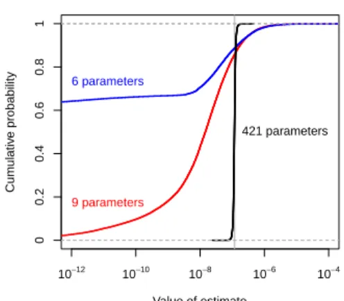
The fact that there is a unique optimum makes it conceivable to find λ∗ us-ing standard optimisus-ing techniques such as Newton and quasi-Newton methods. To do so would require introducing a suitable normalising constraint in order to force the Hessian to be negative definite. In the case of the cross-entropy algorithm of [31], this constraint is inherent because it works at the level of in-dividual transition probabilities that sum to 1 in each state. We note here that in the case that our parameters apply to individual transitions, such that one parameter corresponds to exactly one transition, (22) may be transformed to Equation (9) of [31] by constraining in every visited state x,⟨η(x), λ⟩ = 1. Equa-tion (9) of [31] has been shown in [42] to converge to f∗(for simple unbounded reachability), implying that under these circumstances f (·, λ∗) = f∗and that it may be possible to improve our parametrised importance sampling distribution by increasing the number of parameters. We illustrate this phenomenon in Fig. 3.
Equation (18) leads to the following expression for λk:
λk= ∑N i=1liziui(k) ∑N i=1lizi ∑|ωi| s=1 η(i)k (xs) ⟨η(i)(x s),λ⟩ (20)
In this form the expression is not useful because the right hand side is depen-dent on λk in the scalar product. Hence, in contrast to update formulae based
on unbiased estimators, as given by (16) and in [31, 40], we construct an iter-ative process based on a biased estimator, but having a fixed point that is the optimum: λ(j+1)k = ∑N i=1liziui(k) ∑N i=1lizi ∑|ωi| s=1 η(i)k (xs) ⟨η(i)(xs),λ(j)⟩ . (21)
Equation (21) is the basis of Algorithm 1 and can be seen as an implementation of (20) that uses the previous estimate of λ in the scalar product. As a result, in contrast to previous applications of the cross-entropy method, (21) converges by reducing the distance between successive distributions, rather than by explicitly reducing the distance from the optimum.
5.1. Smoothing
It is conceivable that certain guarded commands play no part in traces that satisfy the property, in which case (21) would make the corresponding parameter zero with no adverse effects. It is also conceivable that an important command is not seen on a particular iteration, but making its parameter zero would prevent it being seen on any subsequent iteration. To avoid this it is necessary to adopt a ‘smoothing’ strategy [31] that reduces the significance of an unseen command without setting it to zero. Smoothing therefore acts to preserve important but as yet unseen parameters. It is of increasing importance as the parametrisation gets closer to the level of individual transition probabilities, since only a tiny proportion of possible transitions are usually seen on any simulation run. Typ-ical strategies include adding a small fraction of the original parameters, or a fraction of the parameters from the previous iteration, to the new parameter estimate. With smoothing parameter α ∈ ]0, 1[, these two strategies can be summarised as follows:
• Weighting with the original parameters:
λ(j+1)k = αµk+ (1− α) ∑N i=1liziui(k) ∑N i=1lizi ∑|ωi| s=1 ηi k(xs) ⟨ηi(x s),λ(j)⟩ (22)
• Weighting with the previous parameters:
λ(j+1)k = αλ(j)k + (1− α) ∑N i=1liziui(k) ∑N i=1lizi ∑|ωi| s=1 ηi k(xs) ⟨ηi(x s),λ(j)⟩ (23)
We have found that our parametrisation is often insensitive to smoothing strat-egy because each parameter typically governs many transitions and most pa-rameters are affected by each run. The smoothing strategy adopted in the case studies described below is to multiply the parameter of unseen commands by 0.95. The effects of this can be seen clearly in Fig. 12. Whatever the strategy, since the parameters are unconstrained it is advisable to normalise them after each iteration (i.e.,∑kλk = const.), in order to judge convergence.
Algorithm 1: Cross-Entropy Algorithm for Parametrised Commands Data:
µ: the original parameters λ(0): the initial parameters
N : the number of paths per iteration
1 j = 0
2 while λ(j) have not converged and j < jmax (see§ 5.4) do
3 A = ⃗0 4 B = 0 5 S = 0 6 for i∈ {1, . . . , N} do 7 ωi = x0 8 li= 1 9 ⃗ui= ⃗0 10 S = 0 11 s = 1
12 while ωi|= ϕ is not decided do
13 generate xs under measure f (., λ(j))
14 ωi = x0· · · xs 15 li← li×µ(xs−1,xs)⟨η i(x s−1),λ(j)⟩ λ(xs−1,xs)⟨ηi(xs−1),λ(j)⟩ 16 update ⃗ui 17 S← S + η i k(xs) ⟨ηi(xs),λ(j)⟩ 18 s← s + 1 19 zi=1(ωi|= ϕ) 20 A← A + liziu⃗i 21 B← B + liziS 22 λ(j+1)k =Ak B 23 λ(j+1)← λ (j+1) ∥λ(j+1)∥ 24 smoothing of λ(j+1) 25 j← j + 1 26 λ∗← λ(j−1)
5.2. Convergence
Theorem 1 proves that there is a unique optimum (λ∗) of (18), which is therefore the unique solution of (20). Equation (21) differs from (20) only in the iteration index of the parameters, hence any fixed point of (21) is also a solution of (20). Since (20) has a unique solution, (21) has a unique fixed point that is the optimum and we conclude that if Algorithm 1 converges, it must con-verge to the unique optimum. We do not provide a formal proof of concon-vergence here, but note that we have never observed divergent or chaotic behaviour in practice. The algorithm is guaranteed to terminate with probability 1 by simply bounding the maximum number of iterations (jmax). The number of samples
per iteration is necessarily finite, so convergence is probabilistic and not neces-sarily monotonic. We typically observe rapid initial convergence that slows to stochastic fluctuations as the parameters approach their optimum values.
The inclusion of smoothing in the algorithm is a practical measure to pre-vent parameters being rejected prematurely when using finite numbers of simu-lations. Smoothing may have the undesirable side effect of slowing convergence and, when using (22), may prevent the algorithm from reaching the theoret-ical optimum. E.g., if the optimal value of λk is ≈ 0, (22) will nevertheless
set λl = αµk. In practice, however, the smoothing strategy is chosen to avoid
problems and have insignificant effect on the final distribution.
Given an adequate initial distribution and sufficient successful traces from the first iteration, (22) and (23) should provide a better set of parameters. In practice we have found that a single successful trace is often sufficient to initiate convergence. This is in part due to the existence of a unique optimum and partly to the fact that each parameter controls a command that usually governs a large number of semantically-linked transitions. The expected behaviour is that on successive iterations the number of traces that satisfy the property increases, however it is important to note that the algorithm minimises the cross-entropy and that the number of traces that satisfy the property is merely emergent of that. As has been noted, in general f (·, λ∗)̸= f∗, hence it is likely that fewer than 100% of traces will satisfy the property when simulating under f (·, λ∗). One consequence of this is that an initial set of parameters may produce more traces that satisfy the property than the final set (see, e.g., Figs. 2 and 10).
Once the parameters have converged it is then possible to perform a final set of simulations to estimate the probability of the rare property. Algorithm 4 describes this process. The usual assumption is that N ≪ NIS ≪ NMC,
however it is often the case that parameters converge fast, so it is expedient to use some of the simulation runs generated during the course of the optimisation (i.e., Algorithm 1) as part of the final estimation.
5.3. Initial Distribution
Algorithm 1 requires an initial simulation distribution (f (·, λ(0))) that
pro-duces at least a few traces that satisfy the property using N simulation runs. Finding f (·, λ(0)) for an arbitrary model may seem to be an equivalently
property (e.g., failure of the system) is semantically linked to an explicit feature of the model (e.g, a command for component failure), good initial parameters may be found relatively easily by heuristic methods such as failure biasing [29]. Alternatively, if the model and property are similar to a previous combination for which parameters were found, those parameters are likely to provide a good initial distribution.
Increasing the parameters associated to commands with obviously small rates may help, along the lines of failure biasing. It is also possible during simulation to make every transition from any given state have equal probabil-ity. In this case parameters are state dependent and calculated on the fly, while the occurrence of commands may still be counted to infer static importance sampling parameters. Note, however, that the rareness of a property expressed in temporal logic may not be related to low transition probabilities. That is, the rareness of a trace (a specific sequence of states) in trace space does not necessarily imply that its transition probabilities are low.
A further important observation is that the rareness of the property in trace space does not imply that good parameters are rare in parameter space. Con-sequently, a random search of parameter space often requires many orders of magnitude fewer attempts to find an example of the rare property than the expected number under the original distribution (i.e., 1/γ). This phenomenon is the basis of the algorithmic approaches to finding initial distributions given below.
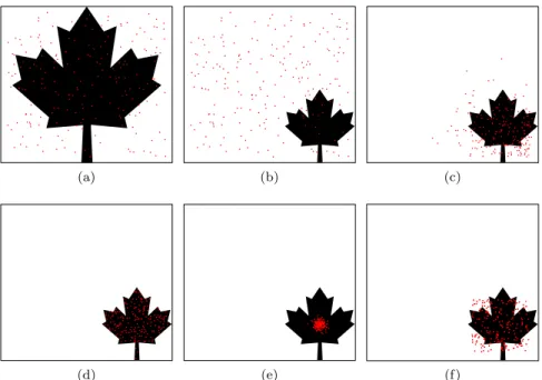
Figure 2 illustrates the parameter space of the chemical model described in Section 6.3. Although the majority of parameters, including those which gener-ate the original distribution (red dot), fall into a region where the probability of satisfying the property is near zero (upper triangle), a significant region of the parameter space (≈ 37%) gives near 100% success (lower triangle). A narrow strip between these two regions (indicated by a grey line in Fig. 2) contains parameters with intermediate levels of success, among which is the unique vec-tor of parameters for minimum cross-entropy. The figure also shows how two different initial parameter vectors converge to the optimum. Although time can-not be discerned from the figure, in both cases the algorithm converges rapidly to the intermediate region, which tends to contain distributions with relatively low cross-entropy. The algorithm then converges more slowly to the point of minimum cross-entropy. In the figure the point is marked by a single blue dot, but since convergence is statistical, the two end points are close but not exactly the same.
5.3.1. Algorithms for Initial Distributions
An effective strategy to find initial distributions is to simulate with ran-dom parameters until a trace satisfying the rare property is observed – the parameters used to generate the trace become λ(0). Note, however, that the
observation of such a trace does not imply that the parameters will necessarily generate satisfying traces with high probability. Choosing parameters in this way is effectively drawing from the joint distribution of parameters and simu-lation traces, hence an individual success may also indicate a high density of
λ1=0 λ2=0
λ3=0 original distribution initial params min C−E params
≈100% success
≈0% success
Figure 2: Parameter simplex of three pa-rameter chemical model.
Value of estimate Cum ulativ e probability 10−12 10−10 10−8 10−6 10−4 0 0.2 0.4 0.6 0.8 1 6 parameters 9 parameters 421 parameters
Figure 3: Importance sampling with increas-ing numbers of parameters.
parameters with relatively low probability of satisfying the property. To account for these eventualities, we give two algorithms.
Algorithms 2 and 3 select parameters uniformly at random by sampling from a Dirichlet distribution with vector of parameters (1, . . . , 1), denoted Dir(1). Algorithm 2 (Optimistic) assumes that the density of parameters is more or less uniform, such that any increase in probability of observing a successful trace is only due to parameters being good. Algorithm 3 (Pessimistic) generalises Algorithm 2 and allows parameters to be judged on their actual performance, rather than relying on the assumption of uniformity. The algorithm performs 1 < N ≪ 1/γ simulation runs per randomly chosen parameter set. The values of N and θ are chosen according to the degree of “pessimism”. N is typically no more than the per-iteration N in Algorithm 1. The value of θ is chosen such that⌈Nθ⌉ ≥ 1 is a realistic expectation of the number of successes.
It is easy to construct pathological examples for which no parameters exist that improve on the original distribution, although we have found this to be unusual with real case studies. If such a case does arise, however, it will be indicated by the number of iterations of Algorithms 2 and 3 performed without success. Under such circumstances, it is useful to note that the probability of success of both algorithms is exactly the probability of the rare event. It is therefore possible to use the reciprocal of the number of simulations as a crude upper bound of γ.
Algorithm 2: Optimistic
z(·) ←model checking function repeat sample λ∼ Dir(1) generate trace ω∼ f(·, λ) until z(ω) = 1; λ(0)← λ Algorithm 3: Pessimistic N ←runs per iteration
θ∈ (0, 1] ←acceptance threshold z(·) ←model checking function repeat sample λ∼ Dir(1) generate N traces ωi ∼ f(·, λ) until∑Ni z(ωi) > N θ; λ(0)← λ 5.3.2. Division of Commands
Our approach exploits the symmetries created by the syntactical definition of the model, under the heuristic assumption that commands link transitions that often have an unambiguous semantic relevance to the property (e.g., indi-vidual commands that govern component failure and repair when considering the property of all components failing). Our guarded commands modelling lan-guage nevertheless allows the guard, rate and action to be complex conditional functions of state variables. When commands have “confused” semantics with respect to the property, parametrisation at the level of the original commands may be too crude. To increase the performance of our approach, it may thus be useful to divide each guarded command into a set of commands with less confused semantics. Without loss of expressiveness, we believe this can be par-tially achieved a priori by restricting the syntax of expressions (e.g., by not allowing conditional actions or rates). We also believe it may be possible to decompose guards automatically. For example, using standard techniques to factorise Boolean expressions, command (guard, rate, action) can be divided into (guard′, rate, action) and (guard′′, rate, action), with guard′∨ guard′′ ≡
guard, guard′∧guard′′≡ false and rate, action unchanged. Additionally, guards
comprising inequalities of the form x < u, with x an integer state variable with lower bound l and u an integer upper bound, are simply divided as follows:
x < u≡∨uk=l−1x = k.
While the automated division of commands remains the subject of future work, we have used this idea to tweak the performance of some of our case studies and to demonstrate the existence of the optimal distribution in a repair model (see Fig. 3).
5.4. The Rare Event Simulation Process
In summary, we run Algorithm 1 to find optimal importance sampling pa-rameters with respect to property φ, then run Algorithm 4 to estimate γ, the probability of φ.
Algorithm 1 is supplied with an initial set of parameters λ(0)that is generated
using one of the procedures described in Section 5.3. The outer ‘while’ loop (line 2) corresponds to the cross-entropy minimisation. This loop terminates when parameters λ(j) converge or when the upper bound of iterations (j
max)
Algorithm 4: Importance sampling by f (., λ∗)
Data:
µ: the original parameters
λ∗: the optimal parameters computed by Algorithm 1
NIS: the number of paths
for i∈ {1, . . . , NIS} do
ωi = x0 li= 1
s = 1
while ωi|= ϕ is not decided do
generate xs under measure f (., λ∗)
ωi = x0· · · xs li← li×µ(xs−1,xs)⟨η i(x s−1),λ(j)⟩ λ(xs−1,xs)⟨ηi(xs−1),λ(j)⟩ s = s + 1 zi=1(ωi|= ϕ) ˜ γ = N1 IS ∑NIS i=1 zili
max0≤k̸=l≤2∥λ(j−k)−λ(j−l)∥ ≤ ϵ. Note, however, that to facilitate comparisons
we simply bound the number of iterations to generate the experimental results reported in Section 6. On line 12, the inner ‘while’ loop is the path generator, in which likelihood ratio liis updated on the fly. On line 16, each time a transition
of type k is taken, the corresponding coordinate of ui is incremented by 1.
Line 23 corresponds to the normalisation of λ(j). On line 24, parameter λ(j) is smoothed by a strategy described in Section 5.1. The resulting parameters are used to generate the new samples.
Algorithm 4 essentially implements the path generating loop of Algorithm 1, but without counting the occurrence of commands.
6. Case Studies
The following case studies are included to illustrate the performance of our algorithms and parametrisation. The principal motivation of statistical tech-niques is to address intractable state space, however the trade-offs between numerical and standard Monte Carlo in this regard are well understood. The particular challenge for our approach is to show that its parametrisation is able to generate good importance sampling distributions. Hence, with the exception of the chemical system, we have chosen models for which we are able to obtain accurate results using numerical techniques, in order to compare the estimates produced by our algorithms with the nominally correct values.
The first case study is a repair model, the second a standard queueing net-work and the third is an example of a chemically reactive system. In the two first cases, initial distributions are created on the fly by assigning equal probability to all enabled transitions from a state. In the third case, an initial distribution
0, 0 1, 0 2, 0 3, 0 4, 0 0, 1 1, 1 2, 1 3, 1 4, 1 0, 2 1, 2 2, 2 3, 2 4, 2 0, 3 1, 3 2, 3 3, 3 4, 3 Failure of type 2 F ailure of typ e 4 9ϵ 6ϵ 3ϵ 9ϵ 6ϵ 3ϵ 9ϵ 6ϵ 3ϵ 9ϵ 6ϵ 3ϵ 9ϵ 6ϵ 3ϵ 4ϵ 3ϵ 2ϵ ϵ 4ϵ 3ϵ 2ϵ ϵ 4ϵ 3ϵ 2ϵ ϵ 4ϵ 3ϵ 2ϵ ϵ 1.5 1.5 1.5 1.5 1.5 1.5 1.5 1.5 1.5 1.5 1.5 1.5 1.5 1.5 1.5 1.5 2 2 2
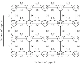
Figure 4: Relationship between failed components of type 2 and type 4 in the repair model. Node labelling gives #type2,#type4. Edgle labelling gives rates of transitions.
is found using Algorithm 2, with fewer than 500 iterations. This value is less than N and considerably less than 1/γ. All simulations were performed using our statistical model checking platform, Plasma [17].
6.1. Repair Model
The need to certify system reliability often motivates the use of formal meth-ods and thus reliability models are studied extensively in the literature. The following example is taken from [31] and features a moderately large state space of 40, 320 states, which can be investigated using numerical methods to corrob-orate our results.
The system is modelled as a continuous time Markov chain and comprises six types of subsystems (1, . . . , 6) containing, respectively, (5, 4, 6, 3, 7, 5) com-ponents that may fail independently. We denote by nu(k) the number of
com-ponents of type k. The system’s evolution begins with no failures and with various stochastic rates the components fail and are repaired. The subsys-tem failure rates are (2.5ϵ, ϵ, 5ϵ, 3ϵ, ϵ, 5ϵ), ϵ = 0.001, and the repair rates are (1.0, 1.5, 1.0, 2.0, 1.0, 1.5), respectively. In addition, components are repaired with priority according to their type. Each subsystem type is modelled by two guarded commands, one for failure and one for repair, using a single variable to count the number of failed components. Figure 4 illustrates the relation-ship between failed components of type 2 and type 4. For simplicity, the other subsystems are not shown.
The property we consider is the probability of a complete failure of a subsys-tem (i.e., the failure of all components of one type), given an initial condition of no failures. This can be expressed in temporal logic as P[X(¬initU1000failure)].
If only one component in the whole system has failed, its immediate repair would violate the property. With this knowledge we are able to make an a priori judicious division of each subsystem’s command for repair. We thus discriminate three cases: (i ) one component of the subsystem has failed and none of the others; (ii ) one component of the subsystem and at least one of another type have failed; and (iii ) at least two components of the same subsystem have failed. Note that the repair command of the components of lower repair priority is just divided into cases (i ) and (iii ), as the second case cannot occur. From an initial 12-command model (six subsystems comprising one command for failure and one command for repair), we constructed a semantically equivalent model of 23 commands (five subsystems comprising one command for failure and three commands for repair and one subsystem comprising one command for failure and two commands for repair). Finally, for each type k, the failure command guard enables the corresponding transitions only if the maximal number of subsystem components nu(k) have not already failed. We split the guard into nu(k) guards,
each of them enabling the transition for a particular number of failed type-k components between 0 and nu(k)− 1. This model contains 47 commands. In
what follows, the three models are denoted r(i, j), with i the number of modules and j the number of commands.
We applied Algorithm 1 to our models, in each case starting from an initial distribution that assigns equal probability to the enabled transitions of any state. We set N = 10000 simulations for each of the 50 cross-entropy iterations, noting that convergence was usually observed in fewer than 20 iterations. The final iteration was used as the importance sampling estimator.
To empirically verify our results we performed each simulation experiment 100 times. Note that the importance sampling estimators are based on NIS =
10000 traces but required a total of 500000 samples. We therefore compare the results of importance sampling with the theoretical values of crude Monte Carlo experiments based on NMC= 500000 samples.
We make use of the concept of skewness, which measures the asymmetry of a distribution X. An unbiased estimator is given by
skew(X) = n (n− 1)(n − 2) ∑n k=1(Xk− ¯x) 3 ( ˆσ2)3/2 , (24)
with ¯x and ˆσ2 the usual unbiased mean and variance estimates.
A skewness close to zero indicates that the estimators are distributed evenly around the mean. A negative value indicates that the distribution is left-tailed (the mass of the estimators is concentrated on the right), while a positive value indicates that the distribution is right-tailed.
For each estimator, we produced a standard approximate 95%-confidence interval CI(ˆγn) = [0.99 (ˆγn− 1.96ˆσn/
√
n) ; 1.01 (ˆγn+ 1.96ˆσn/
√
n)], with ˆσnthe
usual unbiased sample standard deviation estimate. In Table 1 we report the mean value of ˆσn over the 100 experiments in the line labelled σn. This value
is to be compared with the standard deviation of Bernoulli distribution z, as described in Section 3. As the length of the confidence interval is proportional
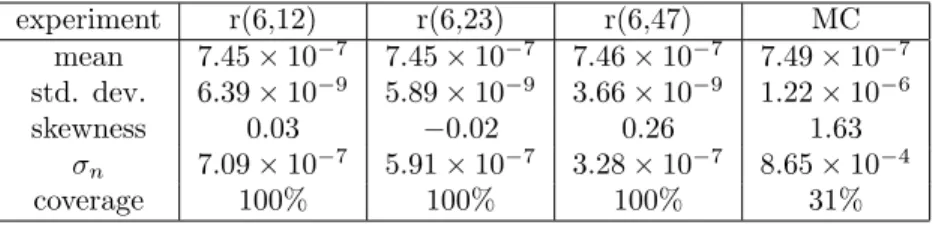
experiment r(6,12) r(6,23) r(6,47) MC mean 7.45× 10⁻⁷ 7.45× 10⁻⁷ 7.46× 10⁻⁷ 7.49× 10⁻⁷ std. dev. 6.39× 10⁻⁹ 5.89× 10⁻⁹ 3.66× 10⁻⁹ 1.22× 10⁻⁶ skewness 0.03 −0.02 0.26 1.63 σn 7.09× 10⁻⁷ 5.91× 10⁻⁷ 3.28× 10⁻⁷ 8.65× 10⁻⁴ coverage 100% 100% 100% 31%
Table 1: Results of repair model
to σn, low ˆσnvalues imply a narrower confidence interval centred around mean
value ˆγn. However, ˆγn remains an estimation of γn. Using values 0.99 and 1.01
is a classic technique to slightly enlarge the approximate confidence interval and increase the chance to strictly fulfil P (γ∈ CI(ˆγn))≥ 0.95. The coverage is the
percentage of approximate confidence intervals that contained the exact value
γ. The expected coverage value is thus expected to be greater than 95%.
In Table 1 we also indicate for the three models the empirical mean, standard deviation, skewness and coverage of the estimates in columns r(6,12), r(6,23) and r(6,47). For comparison, the notional values for Monte Carlo estimates based on NMC= 500000 sample size are given in column MC.
We can see that for all models the cross-entropy algorithm gives a very accu-rate estimate, with variance decreasing with increasing numbers of commands. The skewness shows that the estimates are evenly distributed about the mean. Last but not least, the confidence intervals always contain the exact value and the length of the confidence intervals is maintained narrow due to low σn
val-ues. In contrast, since most of the Monte Carlo estimates are equal to 0, their underlying confidence interval is reduced to 0 at 69%. With probability 31%, they are equal to 1/(5× 10−6) and contain γ but at the price of a very large width.
Figure 12 shows the convergence of parameters for a particular experiment with r(6,12) and highlights the effects of the adopted smoothing strategy. While most parameters converge to stable values, the parameters denoted by green and magenta lines (corresponding to repair of components of types 5 and 6, respectively) are continually attenuated by the smoothing factor (0.95 in this case). Their commands are not seen in successful traces, suggesting that they are less important than the other parameters with respect to the property. Most of the other parameters lie in the approximate range 0.01 to 0.25, but the parameters denoted by red and blue lines (corresponding to the failure and repair, respectively, of components of type 4) are significantly outside. It is clear that increasing the failure rate of components of type 4 is critical to the property. The fact that repair transitions are generally made less likely by the algorithm agrees with the intuition that we are interested in direct paths to failure. The fact that they are not necessarily made zero reinforces the point
that the algorithm seeks to consider all paths to failure, including those that have intermediate repairs.
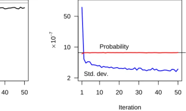
Figure 5 plots the number of paths satisfying X(¬initU1000failure) and
sug-gests that for this model the parametrised distribution is close to the optimum. Figure 6 plots the estimated probability and sample standard deviation dur-ing the course of the algorithm, superimposed on the probability calculated by numerical model checking (horizontal line). The long term average agrees well with the true value (an error of -0.5%, based on an average excluding the first estimate), justifying our use of the sample standard deviation as an indication of the efficacy of the algorithm: our importance sampling parameters provide a variance reduction of more than 106with respect to the variance of the Bernoulli
random variable z (≈ γ). Iteration Number of tr ue paths 1 10 20 30 40 50 8000 10000 9000
Figure 5: Convergence of number of paths satisfying X(¬initU1000failure) in the
re-pair model r(3,12) using N = 10000.
Iteration × 10 − 7 1 10 20 30 40 50 2 10 50 γ Probability Std. dev.
Figure 6: Convergence of empirical mean and standard deviation of likelihood ratio for re-pair model r(3,47) using N = 10000. γ indi-cates true probability.
6.2. Tandem Queueing Network
The following example is adapted from [43] and represents a queueing net-work of two queues of customers (M/Cox2/1-queue and M/M/1) composed sequentially. The system is modelled as a continuous time Markov chain and originally comprises two modules. We add a third passive module whose purpose is to count the number of steps.
Both queueing servers have capacity c = 20. The first desk receives cus-tomers with rate λ = 4c. With probability 0.1, the server of the first desk handles a customer’s request in one phase with rate µ1 = 2; with probability
0.9, the server needs an extra phase to treat the request with rate µ2 = 2. In
this case, an internal variable of the first module, ph is set to 2 instead of 1. Once served, customers leave the first desk and join the queue of the second desk where service occurs with rate κ = 4. If the second queue is full, the first desk is said to be blocked. In this case, the first desk can still pass a request