Localized strain field measurement on laminography data with mechanical regularization

HAL Id: hal-00956440

https://hal.archives-ouvertes.fr/hal-00956440

Submitted on 6 Mar 2014

HAL is a multi-disciplinary open access

archive for the deposit and dissemination of

sci-entific research documents, whether they are

pub-lished or not. The documents may come from

teaching and research institutions in France or

L’archive ouverte pluridisciplinaire HAL, est

destinée au dépôt et à la diffusion de documents

scientifiques de niveau recherche, publiés ou non,

émanant des établissements d’enseignement et de

recherche français ou étrangers, des laboratoires

Localized strain field measurement on laminography

data with mechanical regularization

Thibault Taillandier-Thomas, Stéphane Roux, Thilo F. Morgeneyer, François

Hild

To cite this version:

Thibault Taillandier-Thomas, Stéphane Roux, Thilo F. Morgeneyer, François Hild. Localized strain

field measurement on laminography data with mechanical regularization. Nuclear Instruments and

Methods in Physics Research Section B: Beam Interactions with Materials and Atoms, Elsevier, 2014,

324, pp.70-79. �10.1016/j.nimb.2013.09.033�. �hal-00956440�

Localized strain field measurement on laminography data

with mechanical regularization

Thibault Taillandier-Thomasa,b_{, Stéphane Roux}a_{, Thilo F. Morgeneyer}b_,

François Hilda

a

LMT-Cachan, ENS Cachan/CNRS/UPMC/PRES UniverSud Paris 61 avenue du Président Wilson, 94235 Cachan Cedex, France

b

Mines ParisTech, Centre des Matériaux, CNRS UMR 7633, BP 87 91003 Evry Cedex, France

Abstract

For an in-depth understanding of the failure of structural materials the study of deformation mechanisms in the material bulk is fundamental. In situ synchro-tron computed laminography provides 3D images of sheet samples and digital volume correlation yields the displacement and strain fields between each step of experimental loading by using the natural contrast of the material. Difficul-ties arise from the lack of data, which is intrinsic to laminography and leads to several artifacts, and the little absorption contrast in the 3D image texture of the studied aluminum alloy. To lower the uncertainty level and to have a better mechanical admissibility of the measured displacement field, a regularized digi-tal volume correlation procedure is introduced and applied to measure localized displacement and strain fields.

Keywords: Artifacts, Digital Volume Correlation, Laminography, Regularization, Strain localization

1. INTRODUCTION

Thin sheet structures are widely used in the transportation industry but their failure behavior is not always well understood. The three stages of ductile fracture, namely, void nucleation, growth and coalescence, are established but bulk data are still needed to assess the interaction between damage and strain localization at low levels of triaxiality, as shown in Figure 1. Thanks to the development of 3D imaging and full-field measurement techniques, quantitative data can be obtained to address these issues. Synchrotron X-ray computed la-minography (akin to tomography) allows 3D imaging to be performed at the

Email addresses: thibault.taillandier-thomas@lmt.ens-cachan.fr (Thibault Taillandier-Thomas), stephane.roux@lmt.ens-cachan.fr (Stéphane Roux), thilo.morgeneyer@mines-paristech.fr(Thilo F. Morgeneyer),

micrometer scale for sheet like samples at the cost of additional noise due to the lack of information [1, 2, 3, 4].

Figure _{1: Illustration of typical ductile fracture path of aluminum alloy sheet loaded in} opening mode

The volumes that are naturally contrasted can be used in digital volume correlation (DVC) analyses to measure 3D displacement and strain fields in the bulk. DVC is an extension of 2D digital image correlation [5] to 3D si-tuations [5, 6]. The first implementations of DVC have consisted of registering small interrogation volumes (or subvolumes) to determine their mean rigid body translations [7]. Local rotations have been added later on [8]. The warping of the interrogation volume has also been introduced in DVC codes [9]. All these approaches are referred to as local, since each analysis is local (i.e., at the scale of the interrogation volume) and no kinematic constraint is prescribed between neighboring subvolumes.

Global approaches to DVC have been introduced thereafter [10]. Contrary to local approaches, the displacement field is defined over the whole region of interest. In particular, in many instances, its continuity is enforced a priori. For example, the kinematics associated with finite element discretizations have been considered [10]. If cracks are to be analyzed, enriched kinematics have also been implemented to account for displacement discontinuities [11, 12]. One further step is to regularize the correlation problem by requiring the measured displa-cement field to satisfy mechanical constraints such as the equilibrium [13, 14]. In particular, in areas where the image texture is not sufficiently contrasted, mechanics is utilized to extrapolate the displacement field. If this type of in-formation is not available, then the displacement measurement in these areas would not be possible. This issue is particularly important in 3D imaging as no artificial texture (e.g., secondary particles) can be added without altering the behavior of the studied material.

The aim of the present study is to evaluate the potential of these regularized approaches in the case of little absorption contrast in the 3D images in addition to the fact that complex kinematic fields are sought (i.e., strain localization). The main challenge is related to the fact that if the regularization is too strong, it may smear out the localized region. Conversely, if the regularization is too weak, the DVC calculations may not converge. One additional question is related to the

impact of noise induced by laminography. It was shown that the measurement uncertainty achieved by C8-DVC (i.e., global approach to DVC using 8-noded cubes) reaches levels [4] that are significantly higher than those achieved by analyzing tomographic data [15, 16]. The latter are themselves higher than what is usually observed when dealing with standard 2D images [5, 6].

The paper is organized as follows. The experiment analyzed herein is introdu-ced in Section 2. It deals with the analysis via laminography of a notched sample made of aluminum alloy. Section 3 summarizes the regularized DVC approach to be used to measure displacement fields of the reconstructed volumes. The proposed regularization combines different functionals, which requires scaling to be performed. Associated with a given choice of normalizing displacement fields, new length scales are obtained. Strain resolutions are first determined in Section 4.1. A scaling strategy is proposed to get a almost unique tendency for different trial displacement fields. For the measured displacement field it is possible to determine strain data (Section 4.2). The cumulative total strain fields are shown and the effect of regularization length is assessed in terms of capturing localized strain fields.

2. EXPERIMENT 2.1. Laminography

Synchrotron radiation computed tomography (CT) is a 3D non-destructive technique for objects extended in one direction and thin in the other two di-rections. By inclining the specimen with an angle θ < 90 degrees with respect to the beam direction, a region of interest that expands along two directions can be scanned [1], see Figure 2. This technique is referred to as synchrotron radiation computed laminography (CL). A filtered-backprojection algorithm is then used to reconstruct the 3D volume [1, 2].

Figure_{2: Schematic view of the CT (a) and CL (b) setup with the ESRF parallel beamline} (after [4])

The 3D images utilized herein were obtained at beamline ID19 of the Euro-pean Synchrotron Radiation Facility (Grenoble, France) with a monochromatic beam of 25 keV, with a 65-degree rotation axis inclination angle and 1,500 pro-jections. The reconstructed volumes have a size of 2, 040 × 2, 040 × 2, 040 voxels, with a voxel size of 0.7 µm. More details on the experimental configuration and on analyses of the reconstructed volumes themselves can be found in Refe-rence [17].

2.2. Material and experimental setup

The material used for this study is a commercial Al-Cu aluminum alloy (AA 2198) in T8 condition. The geometry of the flat and notched specimen is schematically shown in Figure 3(a). The 1-mm thick sample (60-mm in width and 70-mm in height) has a notch that has been machined by EDM leading to a radius of 0.17 mm. The loading consists of opening the notch mouth with a displacement controlled by 2-screw device. Stepwise loading has been applied between each laminography scan. An anti-buckling device, which is not shown, has been mounted around the specimen, leaving a window close to the notch to scan the volume close to the notch. From the scanned region, the region of interest for DVC analyses is chosen to be away from the notch root (Figure 3(b)).

(a) (b)

Figure_{3: (a) Schematic view of the analyzed test [4]. The x-axis lies along the thickness of} the plate, the y-axis corresponds to the main propagation direction, and the z-axis is aligned with the load direction. (b) The scanned volume is sketched as a cube delineated in black. The region of interest is a parallelipedic volume away from the notch, which can be seen as a dark region for small y. It is a gray volume limited by white lines for large y

For the analyzed region of interest, the amount of information is quite low, as shown in the histogram of gray level in Figure 4(a) and in the volume with enhanced contrast from Figure 4(b). Further, the inclusion volume fraction is of 0.3-0.4 %. The presence of ring and reconstruction artifacts can be noticed in Figure 4(b) and makes DVC difficult because it has to be based on true microstructure and not on artifactual features. It is interesting to assess the

(a) (b)

Figure_{4: (a) Gray level histogram of (b) the view of the region of interest with an enhanced} contrast to reveal reconstruction artifacts

development of strains and in particular the strain pattern in such type of experiment and its impact on the final damage change. To address this issue, there is a need for reliable kinematic measurements (i.e., displacement and strain fields) in the presence of very poor textures (Figure 4). Once such data are available, the next question to answer is linked with the detection of damage. These two points are solved by resorting to global and regularized digital volume correlation thanks to the measured displacement fields and the corresponding correlation residuals.

3. REGULARIZED DIGITAL VOLUME CORRELATION 3.1. Global DVC

DVC consists of registering two reconstructed volumes, namely, a volume f in the reference configuration, and volume g in the deformed configuration assuming gray level conservation

f (x) = g(x + u(x)) (1) where x is the position of any voxel and u the unknown displacement. Because the strict conservation is not satisfied, especially in CL where noise appears due to reconstruction artifacts due to missing information/angles [3], the correlation residual φc(x) expressed as

φc(x) = |f(x) − g(x + u(x))| (2)

is used in the sum of squared differences Φ2 c = Z ROI φ2 c(x)dx (3)

that is minimized with respect to kinematic unknowns. This problem is ill-posed and nonlinear. Thus a weak formulation based on C8 finite element is chosen in which the displacement is decomposed as

u(x) =X

n

unψn(x) (4)

where un are the degrees of freedom (to be measured) associated with the

trili-near shape functions ψn of C8 elements. By using a modified Newton iterative

procedure [10], linear systems are to be solved

[M]{δu} = {b} (5)

where [M] is the correlation matrix, {δu} the correction to vector {u} gathering all unknown degrees of freedom, and {b} the RHS vector that needs to decrease so that convergence is achieved (i.e., the corrections {δu} become vanishingly small).

3.2. Regularized DVC

Regularization consists of adding some mechanical requirements with ad-ditional functionals, some based on the equilibrium gap method [18], which constrains the displacement field to be the solution to an elastic problem with known body forces

[K]{u} = {f} (6)

where [K] is the stiffness matrix, and vector {f} gathers all the nodal forces. Equilibrium residuals arise for (usually unloaded) inner nodes if u does not satisfy equilibrium. The equilibrium gap functional reads

Φ2 m= {u}

t_[K]t

[K]{u} (7)

When the latter vanishes, equilibrium is strictly satisfied for inner nodes so that mechanical admissibility is satisfied.

The previous strategy cannot be used as such for boundary nodes, except those that belong to a free edge. In that case the previous setting is extended to these particular nodes. For the other boundary nodes, an edge regularization is considered in the same spirit as what was recently proposed for 2D situations [19]

Φ2 b = {u}

t

[L]t[L]{u} (8) where matrix [L] behaves on the ROI boundaries.

These three functionals cannot be added since they do not have the same physical units [14]. Consequently, a reference displacement field v is needed to normalize each functional. The three normalized functionals are dimensionless and thus can be combined. A weight wmand wb is given to functionals Φ

2 mand

Φ2

b, thereby defining regularization lengths that act as cut-off wavelength of low

pass filters [14, 19]. The regularized correlation procedure consists of iteratively solving linear systems

with [N] = wm {v} t_[M]{v} {v}t_[K]t_[K]{v}[K] t_{[K] + w} b {v} t_[M]{v} {v}t_[L]t_[L]{v}[L] t_{[L] (10)}

In the present case, displacement v is associated with a wave of vector k so that the two weights are defined as

wm= wb= (2π|k|ℓr) 4

(11) where ℓr is the regularization length.

Regularization makes use of a constitutive law, which in the present case is that of a linear and isotropic elastic medium. Based on a decomposition of the strain tensor ǫ into a spherical part, ǫsph= (1/3)tr(ǫ)I, and a deviatoric part,

ǫdev= ǫ − ǫsph, the stress tensor σ reads

σ= 3Ktr(ǫ)I + 2Gǫdev (12)

where K (resp. G) is the bulk (resp. shear) modulus, and I the second order identity tensor. The moduli ratio is given by

K G =

2(1 + ν)

3(1 − 2ν) (13)

As Poisson’s ratio ν approaches the incompressibility limit, i.e., ν = 1/2, or ν = 1/2 − η with η → 0, K/G ∼ 1/(2η).

The expression of the equilibrium gap density in the continuum limit reads kdiv(σ)k2

=X

i

((3K + 2G/3)uj,ji+ Gui,jj) 2

(14)

Among the two elastic constants that come into play in this expression, one di-sappears through the normalization (or can be included in the prefactor of Φm).

However, the relative weight of the deviatoric and volumetric strain terms in the sum, which is controlled by K/G, allows for some flexibility in the introduction of the kinematic regularization as discussed below.

Let us stress that this regularization does not necessarily imply that the solid is linearly elastic and described accurately by the above constitutive law. Seen as a mere ad hoc regularization to smooth out high spatial frequencies, it can be shown that the most general form of linear operator acting on the displacement field that is invariant under a rigid body motion (translation and rotation) has precisely the form of Lamé’s operator div(σ). For a solid medium that is loaded away from its elastic limit, a tangent stiffness ∂σ/∂ǫ can be defined, which looks alike the above elastic constant. As will be argued below, as plastic flow occurs at constant volume, a Poisson’s-like ratio close to 1/2 may be chosen to prescribe incompressibility rather than the actual elastic Poisson’s ratio. The actual limitation comes from the assumption of a uniform stiffness, which is generally untrue for nonlinear mechanical behaviors. However, as the mechanical filter affects only the small scales, this inhomogeneity may not have severe consequences unless too much weight is given to the regularization kernel.

4. DVC RESULTS

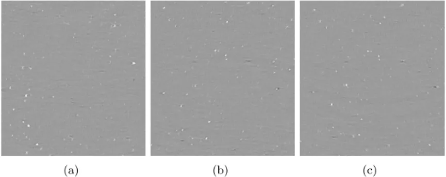
In the sequel, four volumes will be considered. Two volumes in the undefor-med configuration are reconstructed to assess the resolution level of the DVC technique. The third volume has been acquired at an early stage of the test, and the fourth at a later stage. In both latter cases, yielding has already occur-red. Consequently, the cumulative total strain will be reported. Since the elastic strains are very small, the cumulative total strain cannot be distinguished from the cumulative plastic strain peq. The size of the volume of interest (see

Fi-gure 4(a)) is 650 × 450 × 700 voxels, and the region of interest (ROI) for DVC has a size of 448 × 288 × 544 voxels. The discretization is based on C8 elements with an edge size ℓ of 16 pixels. The regularization lengths ℓr considered

he-reafter are equal to 500 voxels (i.e., most of the weight is put on regularization since ℓr ≫ ℓ), 50, 40, 30, 10 and 5 voxels (regularization effects become

negli-gible when ℓr < ℓ). In the early loading stages considered herein, no damage

nucleation on intermetallic particles was observed in the region of interest. This finding stands in contrast to a related study [20] where damage at very brittle particles occurs very early on. However, these particles were of different nature (i.e., Mg2Si) than those found herein (i.e., Fe-based) and of substantially bigger

individual size favoring early fracture/debonding.

(a) (b) (c)

Figure_{5: Slices parallel to the x −z plane taken from the undeformed volume (a), the volume} at early (b) and late (c) stages of the test

4.1. Resolution analysis

The resolution analysis consists of correlating the first two volumes. Very small displacements have occurred between the two acquisitions. However, be-cause of various artifacts, these two volumes are not identical but essentially corrupted by noise. Regularized DVC is run and the results yield nodal displa-cements associated with the finite element discretization. The mean displace-ment gradient in each eledisplace-ment is then evaluated. From the latter, the Green Lagrange strain tensor is computed and its second invariant (i.e., the cumula-tive Von Mises’ strain) is obtained. More details can be found in Reference [21].

The standard deviation of the measured values is reported. It is referred to as standard strain resolution since it corresponds to the largest level below which the measurement can be confused with noise. Three different displacement fields v are considered for the normalization procedure of regularized DVC. The first displacement field involves a change of volume

v0x= v0y = v0z = sin(2πkx) sin(2πky) sin(2πkz) (15)

while the two others are incompressible    v1x= sin(2πky) v1y = sin(2πkz) v1z= sin(2πkx) (16) and    v2x= sin(2πky) sin(2πkz) v2y= sin(2πkx) sin(2πkz) v2z= sin(2πkx) sin(2πky) (17)

where k is a wavenumber equal to 0.1 voxel−1. The aim of the following

ana-lysis is to study the influence of the normalization displacement field on the measurement results.

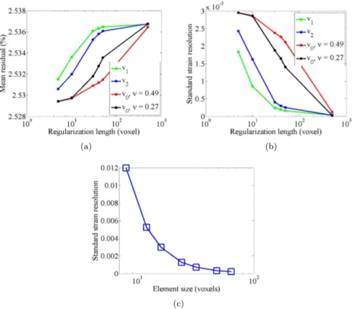
Two different values for Poisson’s-like ratio will be considered (i.e., ν = 0.27 and ν = 0.49). The former corresponds to a rough estimate of the actual Pois-son’s ratio of the studied material. However, since plasticity is likely to occur, a value of Poisson’s-like ratio close to 0.5 allows the displacements to be quasi in-compressible. Figure 6(a) shows the change of the mean correlation residuals, in percent of the dynamic range of the ROI, for the different regularization lengths ℓrand for the four normalizing displacement fields. There is virtually no

varia-tion (note the very small dynamic range in the figure) of the residuals. From a pure correlation stand point, all the results are equivalent and have properly converged.

However, the standard strain resolution shown in Figure 6(b) does not fol-low the same trend. The larger the regularization length ℓr, the smaller the

resolution. As expected [14], the regularization length defines the spatial reso-lution of regularized DVC once it becomes greater than the element size ℓ. The overall trend is identical for any chosen displacement field v. However, the re-lative levels are different. For field v0 two results are reported by using the two

Poisson’s-like ratio values. When ν = 0.49, the deviatoric strain field is very weakly regularized. Therefore it is expected that the strain and displacement fluctuations are larger than those obtained for ν = 0.27. This is observed in Fi-gure 6(b). As the regularization length increases, this effect is more pronounced since the mechanical regularization has a larger weight. Let us note that wha-tever the regularization length and the normalization field, the standard strain resolution is still lower than without regularization for the same element size as can be seen by comparing Figure 6(b) and Figure 6(c).

As the limit of an incompressible material is considered, it is to be emphasi-zed that the reference displacement field v chosen to normalize the regularization

(a) (b)

(c)

Figure_{6: Mean correlation residuals (in percentage of the dynamic range of the volume in} the reference configuration) (a) and corresponding standard strain resolution (b) for different regularization length ℓr and normalizing fields v. (c) Standard strain resolution for different

C8 element sizes without regularization

part may have a very strong weight on the result. Let us consider a dimensional analysis, where terms such as ua,jkare assumed to be of order U/λ2where U is a

characteristic displacement magnitude and λ the characteristic scale over which the displacement varies. If the displacement field is not isochoric, then the order of magnitude of the equilibrium gap is (to dominant order) K2

U2

/λ4

, while if it is divergence-free, the equilibrium gap amounts to G2

U2

/λ4

. The ratio of these two terms is therefore of order 1/η2

.

In fact, there are not one but two regularization lengths. They can be consi-dered as of the same magnitude when ν differs significantly from 0.5. However in the incompressible limit, they have to be distinguished as their ratio diverges. One length is relative to the volume change, ℓsph, while the second is linked to

elastic properties, K/G, and hence ℓsph

ℓdev ≈

1

√_η (18)

In the cases considered below, when ν = 0.49, a factor of 10 is expected in the ratio of these two length scales. The cut-off length that was introduced earlier ℓr will essentially set ℓsph = ℓr if the reference displacement field v

has the volumetric strain of the same magnitude as the equivalent deviatoric strain. However, if the reference displacement field is traceless, then ℓdev= ℓr. It

should be emphasized that the ratio between length scales (see Equation (18)) is independent of the choice of ℓr, and hence changing the reference field from

non-isochoric to isochoric can be exactly compensated for by a corresponding change in ℓr. In terms of displacement field wavelength, λ, three regimes are to

be considered :

– at large wavelength, λ > ℓsph, DVC is the dominant contribution,

– at intermediate wavelength, ℓdev < λ < ℓsph, the DVC functional is

opti-mized in the subspace of isochoric displacement fields,

– at small wavelength, λ < ℓdev, the displacement field has to be the solution

to an elastic incompressible problem. Within this much more constrained choice, image registration decides for the best candidate.

Last, let us also note that the boundary regularization can also be affected if the corresponding length scale is linked to (and, in the present case, even equal to) ℓr.

It is difficult to compare the results given by different normalizations because each of them has a different influence on matrix [N] (see Equation (10)). A way to circumvent this issue is to consider that the main part of the regularization is associated with the equilibrium gap (of inner nodes). An equivalent regulari-zation length ℓreq appears if the weight on that term is equal for a given length

for every displacement field vi considered

wvi,ℓreq m = w vi,ℓri m {vi}t[M]{vi} {vi}t[K]t[K]{vi} {v1}t[K]t[K]{v1} {v1}t[M]{v1} (19) The rescaling is performed by considering the regularization length of v1as a

reference (i.e., for v1, lr= lreq). The effect of the previous rescaling is shown in

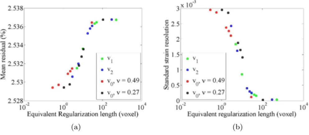
Figure 7. The trends in terms of mean correlation residuals and standard strain resolutions are virtually identical for all four normalizing fields. The fact that the collapse is not perfect is due to the other regularization terms. Figure 7(b) shows that for small equivalent regularization lengths ℓreq, the standard strain

resolution tends to 0.3 %. This level is associated with the resolution of C8-DVC (with an element size ℓ). Conversely, very small resolutions are observed for large equivalent regularization lengths (i.e., less than 10−4) even though the

texture is very difficult.

4.2. Equivalent strain measurement

Now that the uncertainty is assessed, the study will focus on measurements between one of the undeformed volumes and the ones at early and late stages of

(a) (b)

Figure_{7: Mean correlation residuals (in percentage of the dynamic range of the volume in} the reference configuration) (a) and corresponding standard strain resolution (b) for different equivalent regularization lengths ℓreq and normalizing fields v when the rescaling has been

applied

loading. The orientation and position of all the volumes shown are those of Fi-gure 4(a). The mean correlation residual of the different correlations (FiFi-gure 8) is almost the same as the levels obtained in the resolution analysis Figure 7. The same quality of registration is obtained for all the analyses performed he-rein. There is a slight degradation for the last stage of loading when larger regularization lengths are considered.

(a) (b)

Figure_{8: Mean residual for correlations between the undeformed volume and early (a) and} later (b) stages of loading for different equivalent regularization lengths ℓreqand normalizing

fields v when the rescaling has been applied.

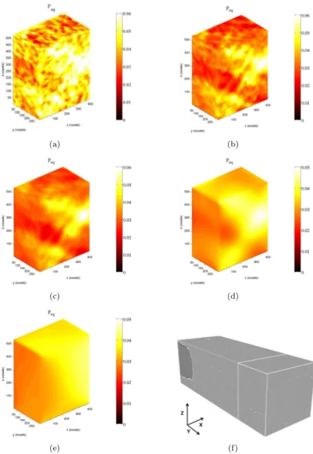
The influence of the equivalent regularization length on the strain fields is shown in Figure 9. If too much weight is put on the regularization (i.e., ℓreq

that is proportional to ℓreq. Strain localization due to plasticity is not properly

captured. This effect explains why the correlation residuals degrade as the equi-valent regularization length increases (Figure 8). Figure 9(b) shows that with a length ℓreq= 30 voxels, which is of the same order of magnitude as the element

size (i.e., ℓ = 16 voxels), many fluctuations of the strain field are filtered out. An equivalent regularization length of ℓreq = 10 voxels seems to be the best

candidate, because the small fluctuation have been filtered out while essentially keeping the same level of residuals and a similar shape of the strain field (Fi-gure 9(c)). Moreover the strain uncertainty, which is less than 0.1%, is more than three times smaller than that obtained without regularization (Figure 7). Larger values of ℓreqcorrespond to a significant increase in the residuals, thereby

indicating that the correlation results are less trustworthy.

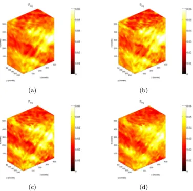
As shown in Figure 8(a), for a small equivalent regularization length close to 5 voxels (i.e., less than the element size), the mean value of the residual field and the equivalent strain field shown in Figure 10, is almost the same regardless of the displacement field used for the normalization procedure. This result can be explained by the fact that a low weight is put on the regularization part compared to the one put on the correlation itself. However, the strain resolution shown in Figure 7(b) for each normalization and regularization length is different.

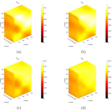
For the later stage of loading and an equivalent regularization length of the same order as the element size (i.e., 30 voxels as indicated in Figure 8(b)), the mean value of the residual field and the equivalent strain fields (Figure 11(a,b)) for v1 and v2 are similar. For v0, the incompressibility is prescribed by the

like ratio, thus the equivalent strain field obtained with a Poisson’s-like ratio of 0.49 (Figure 11(c)) looks Poisson’s-like the ones of v1 and v2. However the

mean value of the residual field, Figure 8(b), is higher.

5. CONCLUSIONS

Using computed laminography in situ experiments have been performed on plate-like specimen with sub-micrometer spatial resolution. The 3D images have then been successfully registered by regularized digital volume correlation to measure displacement and strain fields in spite of very little contrast due to a low content of particle used as markers. This is the case of the aluminum alloy that was analyzed herein.

To lower the measurement uncertainties, a regularization procedure was fol-lowed. Within the framework of global approaches to digital volume correlation, it consists of prescribing additional constraints on inner nodes (i.e., minimiza-tion of the equilibrium gap) and boundary nodes (i.e., minimizing displacement fluctuations). The weight put on various regularization terms translates into regularization lengths that can be compared to the underlying finite element discretization. The standard strain resolution could be decreased from an initial level of 0.3 % (for 16-voxel elements) to less than 0.01 % for large regularization lengths (i.e., greater than 100 voxels).

(a) (b)

(c) (d)

(e) (f)

Figure _{9: Equivalent strain for the early stage of loading without regularization (a) and} with the normalizing displacement field v1 and different equivalent regularization lengths

ℓreq= 5voxels (b), ℓreq= 10voxels (c), ℓreq= 30voxels (d), and ℓreq= 500voxels (e). (f)

Frame and location of the region of interest

It is worth noting that the regularization length corresponds to the cut-off length of a low pass mechanical filter. Special care should be exercised when

(a) (b)

(c) (d)

Figure_{10: Equivalent strain for the early stage of loading with an equivalent regularization} length of 5 voxels (see Figure 8(b)) that corresponds for field v1 to a length of 5 voxels (a),

about 5 voxels for field v2 (b), 30 voxels for field v0 with Poisson’s ratio of 0.49 (c), and 50

voxels for the Poisson’s ratio of 0.27 (d). The frame is identical to that of Figure 9(f)

localization phenomena are studied. If a too large regularization length is se-lected, the kinematic fields are no longer faithfully evaluated. Conversely, when too small regularization lengths are chosen, measurement uncertainties become more pronounced. Consequently a trade-off is needed to account for these two opposite effects. Last, the mechanical regularization used herein is based on elastic assumption for the underlying behavior of the analyzed material. This limitation was partially circumvented by assuming quasi isochoric displacement and strain fields. However, to better capture localized bands other routes may be followed.

The method developed herein reveals to be viable for the study of complex strain patterns arising during ductile tearing. Larger regions are to be studied and the entire load history up to fracture to be analyzed to gain new insight into the ductile failure mechanisms at play.

6. ACKNOWLEDGEMENTS

Fédération Francilienne de Mécanique is thanked for its support and Constel-lium CRV for material supply. The authors acknowledge ESRF for providing

(a) (b)

(c) (d)

Figure_{11: Equivalent strain for the late stage of loading with an equivalent regularization} length of 30 voxels (see Figure 8(b)), which corresponds for field v1to a regularization length

of 30 voxels (a), 50 voxels for field v2 (b) and 500 voxels for field v0 with Poisson’s ratio of

0_{.49(c) or 0.27 (d). The frame is identical to that of Figure 9(f)}

beamtime (experiment MA1006). L. Helfen and X. Fu are gratefully acknowled-ged for his invaluable help with the laminography experiments.

7. REFERENCES

[1] L. Helfen, T. Baumbach, P. Mikulik, D. Kiel, P. Pernot, P. Cloetens, and J. Baruchel. High-resolution three-dimensional imaging of flat objects by synchrotron-radiation computed laminography. Appl. Phys. Lett., 86 : 071915, 2005.

[2] L. Helfen, T. Baumbach, P. Cloetens, and J. Baruchel. Phase contrast and holographic computed laminography. Appl. Phys. Lett., 94, 2009.

[3] F. Xu, L. Helfen, T. Baumbach, and H. Suhonen. Comparison of image qua-lity in computed laminography and tomography. Optics Express, 20 :794– 806, 2012.

[4] T.F. Morgeneyer, L. Helfen, H. Mubarak, and F. Hild. 3D Digital Volume Correlation of Synchrotron Radiation Laminography images of ductile crack initiation : An initial feasibility study. Exp. Mech, 53(4) :543–556, 2013.

[5] M. A. Sutton, J.-J. Orteu, and H. Schreier. Image correlation for shape, motion and deformation measurements : Basic Concepts, Theory and Ap-plications. Springer, New York, NY (USA), 2009.

[6] F. Hild and S. Roux. Optical Methods for Solid Mechanics. Section Digi-tal Image Correlation : Problem Solutions. P. Rastogi and E. Hack, eds., Wiley-VCH, Weinheim (Germany), 2012 :183–228, 2012.

[7] B. K. Bay, T. S. Smith, D. P. Fyhrie, and M. Saad. Digital volume cor-relation : three-dimensional strain mapping using X-ray tomography. Exp. Mech., 39 :217–226, 1999.

[8] T. S. Smith, B. K. Bay, and M. M. Rashid. Digital volume correlation including rotational degrees of freedom during minimization. Exp. Mech., 42 :272–278, 2002.

[9] E. Verhulp, B. van Rietbergen, and R. Huiskes. A three-dimensional digital image correlation technique for strain measurements in microstructures. J. Biomech., 37 :1313–1320, 2004.

[10] S. Roux, F. Hild, P. Viot, and D. Bernard. Three dimensional image cor-relation from X-ray computed tomography of solid foam. Comp. Part A, 39 :1253–1265, 2008.

[11] J. Réthoré, J.-P. Tinnes, S. Roux, J.-Y. Buffière, and F. Hild. Extended three-dimensional digital image correlation (X3D-DIC). C. R. Mécanique, 336 :643–649, 2008.

[12] J. Rannou, N. Limodin, J. Réthoré, A. Gravouil, W. Ludwig, M.-C. Baïetto, J.-Y. Buffière, A. Combescure, F. Hild, and S. Roux. Three dimensional experimental and numerical multiscale analysis of a fatigue crack. Comp. Meth. Appl. Mech. Eng., 199 :1307–1325, 2010.

[13] H. Leclerc, J-N. Périé, S. Roux, and F. Hild. Voxel-scale digital volume correlation. Exp. Mech, 51(4) :479–490, 2011.

[14] H. Leclerc, J-N. Périé, F. Hild, and S. Roux. What are the limits to the spatial resolution ? Mechanics & Industry, 13 :361–371, 2012.

[15] N. Limodin, J. Réthoré, J.-Y. Buffière, A. Gravouil, F. Hild, and S. Roux. Crack closure and stress intensity factor measurements in nodular graphite cast iron using 3D correlation of laboratory X-ray microtomography images. Acta Mat., 57 :4090–4101, 2009.

[16] N. Limodin, J. Réthoré, J. Adrien, J.-Y. Buffière, F. Hild, and S. Roux. Analysis and artifact correction for volume correlation measurements using tomographic images from a laboratory X-ray source. Exp. Mech., 51 :959– 970, 2011.

[17] T.F. Morgeneyer, L. Helfen, I. Sinclair, H. Proudhon ans F. Xu, and T. Baumbach. Ductile crack initiation and propagation assessed via in situ synchrotron radiation computed laminography. Scripta Mat., 65 :1010– 1013, 2011.

[18] D. Claire, F. Hild, and S. Roux. A finite element formulation to identify damage fields : The equilibrium gap method. Int. J. Num. Meth. Eng., 61(2) :189–208, 2004.

[19] Z. Tomicevic, S. Roux, and F. Hild. Mechanics-aided Digital Image Corre-lation. J. Strain Analysis, 48 :330–343, 2013.

[20] Y. Shen, T. F. Morgeneyer, J. Garnier, L. Allais, L. Helfen, and J. Crépin. Three-dimensional quantitative in situ study of crack initiation and propa-gation in aa6061 aluminum alloy sheets via synchrotron laminography and finite-element simulations. Acta Mat., 61[7] :2571–2582, 2013.

[21] F. Hild, E. Maire, S. Roux, and J.F. Witz. Three-dimensional analysis of a compression test on stone wool. Acta Mat., 57 :3310–3320, 2009.