HAL Id: hal-00512104
https://hal.archives-ouvertes.fr/hal-00512104
Submitted on 27 Aug 2010
HAL is a multi-disciplinary open access
archive for the deposit and dissemination of
sci-entific research documents, whether they are
pub-lished or not. The documents may come from
teaching and research institutions in France or
abroad, or from public or private research centers.
L’archive ouverte pluridisciplinaire HAL, est
destinée au dépôt et à la diffusion de documents
scientifiques de niveau recherche, publiés ou non,
émanant des établissements d’enseignement et de
recherche français ou étrangers, des laboratoires
publics ou privés.
A compromise definition in multiobjective
multidisciplinary design optimization
Benoît Guédas, Philippe Dépincé
To cite this version:
Benoît Guédas, Philippe Dépincé. A compromise definition in multiobjective multidisciplinary
de-sign optimization. 8th World Congress on Structural and Multidisciplinary Optimization, Jun 2009,
Lisbonne, Portugal. �hal-00512104�
8th
World Congress on Structural and Multidisciplinary Optimization
June 1-5, 2009, Lisbon, Portugal
A compromise definition in multiobjective multidisciplinary design
optimization
Benoˆıt Gu´edas and Philippe D´epinc´e
IRCCyN, Nantes, France
{benoit.guedas,philippe.depince}@irccyn.ec-nantes.fr
1. Abstract
The decomposition of a global problem into several sub-problems, that can have antagonist goals, requires to find trade-off solutions. Moreover, the sub-problems are often multi-objective optimization problem : the disciplines have several antagonist objectives to optimize simultaneously. Thus, trade-off solutions have to be found both at the discipline level and at the multidisciplinary level. One way to consider the compromise is to compute all the Pareto efficient solutions of the multi-objective problem involving all the objectives of the disciplines at the same time. The optimal solutions can then be defined as the direct product of each disciplines partial ordered set by Pareto dominance relation. Unfortunately, this defini-tion of the compromise is not satisfying. Indeed, informadefini-tion about efficiency of the soludefini-tions inside each discipline is lost during the direct product. In this paper, we propose extensions of the partial ordered set defined by the Pareto dominance relation in each discipline that keeps this information. Another dominance relation over disciplines is also presented.
2. Keywords: multidisciplinary, multiobjective, optimization, compromise. 3. Introduction
The growing complexity of industrial products have led to specialization and distribution of knowledge, tools and work sites. The designer have now to face two main problems : the optimization of the product quality on a first hand, and the organization of work on a second hand. Multidisciplinary design optimization deals with all the problems that can arise in this context. For example, the optimization of the wing of an aircraft is both an aerodynamic and a structural problem in which each discipline have its own objective and uses specific tools, but a global solution have to be found. The decomposition of a global problem into several sub-problems, that can have antagonist goals, requires to find trade-off solutions. Moreover, the sub-problems are often multi-objective optimization problems: the disciplines have several antagonist objectives to optimize simultaneously. Thus, trade-off solutions have to be found both at the discipline level and at the multidisciplinary level.
In multiobjective multidisciplinary related papers, the compromise is not clearely defined and cor-responds in fact to the Pareto optimal solution of the global problem including all the objectives of all the disciplines at the same time. This compromise is relevant if the decomposition of the problem in several disciplines is only due to practical organisational aspects. In the case where the decomposition in disciplines corresponds to a hierarchical organisation of the decision process, the global Pareto front may not represent the expeted compromise. For instance if there exists a subset of solutions that are optimal for all the disciplines at the same time, the global Pareto front will not be this subset of solutions but a larger set including solutions that are not optimal for all the disciplines. We propose a compromise method which in this situation only gives the subset of solutions that are optimal for all the disciplines at the same time. More generally, the proposed compromised method is not a compromise among the objectives but among disciplines.
As we are looking for a compromise method among disciplines which are optimization problems, the fourth section defines what are the solution of an optimization problem - and in particular a multiobjective optimization problem. This section introduces the notations and concepts used along this paper. The solutions are defined using ordered sets theory. The fifth section then defines our compromise method using the orederd set definitions and operations presented in the previous section. Finally, properties and examples of the proposed compromise are given in the sixth section before conclusions.
In some multidisciplinary design optimization problems, some variables are shared bewteen several disciplines while others are local to a given discipline. Moreover, many of these problems are coupled: inputs of one discipline are outputs of another discipline and vice versa. As this paper is a first attempt
to define compromise bewteen disciplines, we only consider a simplified problem were all the disciplines share the same set of design variables and have no coupling functions.
4. Solutions of an optimization problem
Before defining a compromise between optimization problems, we need to define what are the solu-tions of an optimization problem. The following definisolu-tions are common to all optimization problems. According to Matthias Ehrgott [4], an optimization can be described by five elements:
• the feasible set X • the objective space E
• the objective function vector f := (f1, . . . , fp) :X → E
• the ordered set (F, ≤) • the model map θ : E → F
An optimization problem is then caracterized by:
(X , f, E)/θ/(F, ≤)
Most of the multidisciplinary design optimization methods such as MDF, IDF, AAO, CO, CSSO, BLISS, ATC,. . . only consider disciplines having one objective. In this case, in each discipline E = R, θ = id (the identity function) and (F,≤) = (R, ≤) the canonical ordered set over the real numbers. Other methods such as E-MMGA, MORDACE and COSMOS are specially designed to handle multiobjective disciplinary problems. Here E = Rn with n
≥ 2 and the solutions are compared with the Pareto-dominance relation . Classical method can also be applied to multiobjective problems if we take a model map θ : Rn
→ R, such as, for instance, the weighted sum : (x1, . . . , xn) 7→ Pni=1ωixi with the
weights ωi∈ R.
The set of solutions of an optimization problem will depend on the choice of the ordered set in which the solutions are compared.
4.1. Partial ordered sets
We give here some definitions about partial ordered sets which will be usefull for the definition of the compromise. More definitions can be found in [10]. To define the minimum of a set, we need to compare pairwise all the points of the set in order to find which of them is minimal. This comparison is an order relation and is defined as follows :
Definition An order relation≤ on a set E is a binary relation verifying the following properties : i) reflexivity: ∀x ∈ E, x ≤ x
ii) antisymetry: ∀x, y ∈ E, x ≤ y ∧ y ≤ x ⇒ x = y ii) transitivity: ∀x, y, z ∈ E, x ≤ y ∧ y ≤ z ⇒ x ≤ z
(E,≤) is then called an ordered set, partial ordered set or poset.
An ordered set in which the elements are comparable given an order relation. Unfortunately, it does not mean that all the elements of the set are comparable but only a subset of them.
Definition Let e1 et e2 be two posets (E,≤). We say that e1 and e2 are comparable, and we write
e1∼ e2et e2∼ e1 if and only if e1≤ e2ou e2≤ e1. We write e1≁ e2if e1 and e2are not comparable.
A set where all the elements are comparables is said totally ordered. (R,≤) is a totally ordered set. Definition Let (E,≤) be an ordered set. ≤ is said total if ∀(e1, e2)∈ E2, e1≤ e2∨ e2≤ e1.
To each order relation, we can associate its strict relation by removing the reflexivity property. In such a relation, an element cannot be compared to itself.
Definition A strict order relation < on a set E is a binary relation verifying the following poperties : i) irreflexivity: ∀x ∈ E, x ≮ x
ii) transitivity: ∀x, y, z ∈ E, x < y ∧ y < z ⇒ x < z (E, <) is then called a strict ordered set.
Some operations such as the sum and the product can then be defined on the ordered sets. Definition Let O1= (E1,≤E1) and On = (En,≤En ) n two ordered sets, et E =
Qn
i=1Ei. We define
the product O =Qn
i=1Oi such that :
e≤Ee′ ⇔ ∀i ∈ {1, . . . , n}, ei≤Ei e′i
Definition Let Q the chain Ch= y1< . . . < yhof h elements. Let h posets Pi = (Xi,≤i). We say that
P = (X,≤P) is the linear sum Pi and we write
P = h M i=1 Pi with : X = h [ i=1 Xi and a≤P b⇐⇒ ( a∈ Xi, b∈ Xj and a≤i b if i = j a∈ Xi, b∈ Xj and yi<Qyj otherwise
In an optimization problem, we are looking for the minima of a poset.
Definition Let (E,≤) be a poset. An element e∗∈ E is said to be minimal iff ∀e ∈ E withe∗∼ e, e∗≤ e.
The set of all minimal elements of E is then written min E.
The minimal elements of (E,≤) can be defined with these to equivalent definitions :
min E = {e∗∈ E : ∀e ∈ E s.t. e∗∼ e, e∗≤ e} (1)
min E = {e∗∈ E : ∀e ∈ E, e ≤ e∗⇒ e∗= e} (2)
We can now define the rank of an element in a poset which is an application from E into N that to each element of a partial ordered set assigns an integer.
Definition Let P = (E,≤) a poset. For x ∈ X, we define the rank r(x) of x such that • r(x) := 0, if x is a minimum.
• r(x) := n, if the elements of rank < n have been assigned and x is a minimum in the poset P\{y ∈ P : r(y) < n}.
The rank can also begin to 1 instead of 0.
4.3. Optimal and efficient solutions
LetX be the feasible set of the decision space of an optimization problem, and Y be its image under the objective function mapping f :X → Rn.
Y is thus a subset of Rn.
Y := {f(x) : x ∈ X } (3)
The solutions of a multiobjective optimization problem are defined with the Pareto-dominance relation ≻ which represent a preference. For a minimization problem we have the following definition of the Pareto-dominance relation:
Definition Let a, b∈ Y ⊆ Rn, we say that a Pareto-dominates b and we write a
≻ b if a is lower than b on each component and if there is at least one component which is strictly lower :
a≻ b ⇐⇒ (
∀i ∈ {1, . . . , n} ai≤ bi
∃j ∈ {1, . . . , n} aj < bj
The Pareto-dominance relation allows us to define the non dominated setYN ⊆ Y which is the set of
all the points of the objective space which are not dominated.
YN :={y∗ ∈ Y : ∄y ∈ Y s.t. y ≻ y∗} (4)
The set of the solutions of the problem is called the efficient set XE ⊆ X and is defined as the set of
points of the feasible set for which their image in the objective space is not dominated.
XE:={x ∈ X : f(x) ∈ YN} (5)
We can notice that the Pareto-dominance relation is similar to the definition of the product of orders but without the reflexivity property (because of the strict order relation). Thus, the Pareto dominance relation is the strict order associated to the direct product. For this reason, we will now us the symbol instead of ≻ for the Pareto-dominance relation.
The solutions of a multiobjective minimization problem can then be interprated as the minima ofY with the order relation of the product (R,≤)n :
YN := {y∗∈ Y : ∀y ∈ Y s.t. y∗∼ y, y∗≤ y} (6)
YN := {y∗∈ Y : ∀y ∈ Y, y ≤ y∗⇒ y∗= y} (7)
The two above definitions of YN are equivalent to the previous one. YN is also called the Pareto
front andXE the Pareto set .
5. Compromise between optimization problems 5.1. Na¨ıve definition
Let X1
E andXE2 be the respectively the efficients sets of the first and the second discipline, and let
Y2
N andYN2 be the corresponding non-dominated sets. Let XE the efficient set of the multidisciplinary
problem and XG
E the efficient set of the global multiobjective optimization problem including all the
objectives. We would like that the efficient soltions of the problem have at least these two properties: 1. a compromise solution belongs to the Pareto front of the global optimization problem,
2. if there are efficient solutions that are common to all disciplines at the same time, then this set of solution is exactly the set of efficient solutions of the multidisciplinary problem.
This can be translated as: 1. XE⊆ XEG
2. X1
E∩ XE2 6= ∅ ⇒ XE=XE1∩ XE2
5.2. The product for compromise
The compromise solutions between n mono-objetive problems is the Pareto set. In other words, the compromise is defined as the minimal solutions of the product of the natural order of R: (R,≤)n.
We can define the compromise between p disciplines which have qi, i∈ {1, . . . , p} objectifs each the
same way: by the product of the p orders (Rqi,
≤Rqi) of each disciplines. Unfortunately, if we sum all the
objectives of all the disciplines and call n the result: n =Pp
(Rn, ≤Rn) = p Y i=1 (Rqi, ≤Rqi) (8)
This equation means that the result of the product of the p disciplines is the same than the product of the n objectives of the problem.
5.3. Extension of the direct product
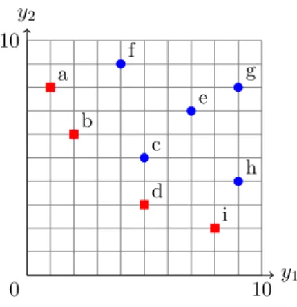
The previous definition is not satisfying because the information on the efficiency of the solutions are lost during the product. Indeed, we can consider that de non-diminated points of each disciplines are better than the others. But a non-dominated point is not always comparable to a dominated point. Then, during the product, if a non-dominated point and a dominated point are not comparable, they are potentially on the global Pareto front if they are also incoparable in other disciplines.
y1 y2 a b c d e f g h i 0 10 10
Figure 1: Tous les points deYN (rouges) sont meilleurs que ceux deYD (bleus)
We want the optimal solutions of a discipline be better than all the other solutions. We can make the two following comments:
1. all the optimal solutions of a discipline are equivalent, 2. an optimal solution is prefered to a non-optimal solution.
LetYD:=Y\YN be the set of dominated points of a discipline. We can define the new order relation≤′
including the two previous comments: 1. ∀(y1, y2)∈ Y, y1≤ y2⇒ y1≤′y2
2. ∀(y1, y2)∈ YN × YD, y1≤′y2
The second point is useless because if all the non-dominated points are equal, by transitivity, they dominate all the other solutions. If the first point is removed and the second one kept, the global Pareto front after the product would be the union of each Pareto front.
We can also extend this new order relation by applying the same argument to all the ranks of the ordered set. We define the new relation≤′′ as follows:
a≤′′b⇐⇒ r(a) ≤ r(b)
Many other definitions of the “rank” have been proposed in the litterature related to multiobjective genetic algorithm. Goldberg [8] first introduced the rank to bias the selection operator based on the evaluations of the objective function. This idea has then been used by Srinivas and [11] Deb in the NSGA algorithm in order to sort the individuals for a multiobjective problem. Other sorting method have been proposed for multiobjective genetic algorithm. But even if they use the term “rank”, they do not correspond to the definition of the rank on a poset. That is why we introduce two new definitions: classification and pseudo-classification to name this mappings.
Definition A classification is a mapping c from the set X into N∗ such that:
• if X 6= ∅, ∃x ∈ X s.t. c(x) = 1
• ∀x1∈ X s.t. c(x1) > 1,∃x2∈ X s.t. c(x2) + 1 = c(x1)
Definition A pseudo-classification is a mapping ϕ from the set X into N∗ such that:
• if X 6= ∅, ∃x ∈ X t.q. ϕ(x) = 1
• ∀x1∈ X s.t. ϕ(x1) > 1,∃x2∈ X s.t. ϕ(x2) + 1≤ ϕ(x1)
The pseudo-classification proposed by Belegund and Salagame [2] assigns the value 0 to each element of the non-dominated set and 1 to each element of the dominated set. The pseudo-classification proposed by Fonseca and Fleming [6] assigns to each element of the objective space the number of individuals it dominates plus one. In ordered sets theory, it corresponds to the cardinality of the ideal. Alberto and Ascarate [1] also proposed two pseudo-classifications. The first one is based on the number of times an element dominated others with random weighted sums, and the second one is a mix between the rank and Fonseca and Fleming’s pseudo-classification.
All the above pseudo-classifications can be used to define the new order ≤′′. We notice that the
first extension≤′ can be interpreted as the second one≤′′with taking Belegund and Salagame
pseudo-classification instead of the rank.
The first compromise bewteen p disciplines is define as follows: YN := min p Y i=1 (Yi N ⊕ Y i D) (9)
More generally, it can be defined as:
YN := min p Y i=1 qi M j=1 ψj(Yi) (10)
with ψi a function that gives the part of a set which has all its elements scored i by the
peudo-classement ϕ:
ψi(E) :={e ∈ E : ϕ(e) = i} (11)
Of course, we can choose ϕ = r.
6. Examples and properties
Let us call c0 the compromise corresponding to the Pareto-optimal solutions of the whole problem, c1 the first compromise proposed and c2 the second one.
6.1. Examples
The second and third examples come from [3]. The fourth and fifth example come from [5]. Example #1 Example #2 D1 min xc,x1 f1(xc, x1) = 10(x1− 0, 1)2+ (xc− 3)2 min xc,x2 f2(xc, x2) = 10(x2− 0, 3)2+ (xc− α)2 D2 min xc,x3 f1(xc, x3) = 10(x3− 0, 3)2+ (xc− β)2 min xc,x4 f2(xc, x4) = 10(x4− 0, 5)2+ (xc− 9)2 With α, β ∈ R Example #3
Objectives f1 f2 a (2,7) (7,7) b (5,5) (4,3) c (6,2) (3,6) d (3,3) (8,5) e (8,7) (2,8) f (7,6) (5,8) D1 min x1,x2 f1(x1, x2) = (x1− 2)2+ (x2− 1)2 min x1,x2 f2(x1, x2) = x21+ (x2− 3)2 D2 min x1,x2 f1(x1, x2) = (x1− 1)2+ (x2+ 1)2 min x1,x2 f1(x1, x2) = (x1+ 1)2+ (x2− 1)2
Under the following constraints:
(x21− x2)≤ 0 (x1+ x2− 2) ≤ 0 (−x1)≤ 0 Example #4 V (x) = L(2x1+ √ 2x2+ √ 2x3+ x4) d1(x) = F L E ( 2 x1 +2 √ 2 x2 − 2√2 x3 + 2 x4 ) d2(x) = F L E ( 2 x1 + 2√2 x2 + 4√2 x3 + 6 x4) d3(x) = F L E ( 6√2 x3 + 3 x4 ) C x1≥ F σ x2≥ √ 2F σ x3≤ 3 F σ x4≤ 3 F σ with: F = 10kN, L = 200cm, E = 2.105kN/cm2
and σ = 10kN/cm2.The deproblem is decomposed into three subproblems as follows: f1= (d1, V ), f2= (d2, V ), f3= (d3, V ) under the constraints C.
6.2. Inclusion
The order relation ≤′′ is an extension of ≤′ which is itself an extention of ≤. Thus, the solutions
for the compromise c2 are all included in the solutions for the compromise c1 which are included in the compromise c0 (global Pareto front). We have the following inclusions:
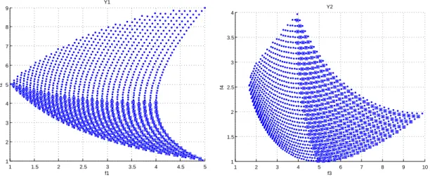
min p Y i=1 qi M j=1 ψj(Yi)⊆ min p Y i=1 (Yi N ⊕ Y i D)⊆ min p Y i=1 Yi N (12) Exemple Rabeau.
1 1.5 2 2.5 3 3.5 4 4.5 5 1 2 3 4 5 6 7 8 9 f1 f2 Y1 1 2 3 4 5 6 7 8 9 10 1 1.5 2 2.5 3 3.5 4 f3 f4 Y2
Figure 2: Our compromise en problem #3
f(1,1) f(1,2) a1 b1 c1 d1 e1 f1 0 10 10 f(2,1) f(2,2) a2 b2 c2 d2 e2 f2 0 10 10
Figure 3: Exemple : tous les points sauf f sont efficaces.
f(1,1) f(1,2) a1 b1 c1 d1 e1 f1 0 10 10 f(2,1) f(2,2) a2 b2 c2 d2 e2 f2 0 10 10
Figure 4: Exemple : seul c est efficace.
Intuitivelly, for two disciplines, Y1
N and YN2 are respectively the Pareto fronts of disciplines 1 and 2
corresponding to their objectives f1and f2. If we callYN−1:= f2(XE1) andYN−2 := f1(XE1) the projection
of each Pareto front in the other discipline, we can say that if there is a solution for which its image is aboveY−1
N orYN−2 in respectively the first and second discipline, then this solution is not a compromise
according to our definition.
Proposition Let i and j two disciplines, i, j∈ {1, 2}, i 6= j. If a solution x1∈ X is such that ∃x2∈ XEj
such that fi(x2) fi(x1), this is not a trade-off solution.
Proof ∃x2∈ XEj such that fi(x2) fi(x1) and x2∈ XEj implies that ∄x3∈ X such that fj(x2) fj(x3).
Thus fj(x2) fj(x1) and so there is at least one solution x2 that dominates x1.
But unfortunately, the opposite is not true: a solution for which both of its images are under Y−1 N
andY−2
N is not always a compromise.
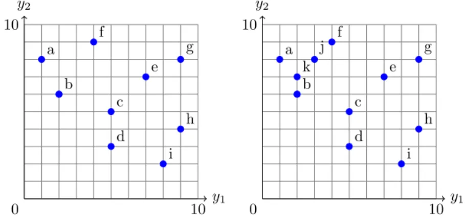
6.4. Stability
Unfortunately, an order based on a pseudo-classification in a partially ordered set is not stable with the spread of the elements in the set. If some elements are added, the order can change as the Fig. 5 shows. y1 y2 a b c d e f g h i 0 10 10 y1 y2 a b c d e f g h i j k 0 10 10
Figure 5: The order between e and f has been reversed.
7. Conclusions
8. References
[1] I. Alberto, C. Azcarate, F. Mallor, and P.M. Mateo, Multiobjective evolutionary algorithms. pareto ranking, Monografias del Seminario Matematico Garcia de Galdeano, vol.27, pages 25–35, 2003. [2] A.D. Belegund and R.R. Salagame, Optimization of laminated ceramic composites for minimum
residual stress and cost, Microcomputers in civil engineering, 10(4):303–306.
[3] P. D´epinc´e, S. Rabeau, and F. Bennis, Collaborative optimization strategy for multi-objective design, In Proceedings of DETC’2005, pages 24–28, September 2005.
[4] M. Ehrgott, Multicriteria Optimization, Springer Berlin / Heidelberg, 2 edition, 2005.
[5] A. Engau and M. M. Wiecek, 2D decision-making for multicriteria design optimization, Structural and Multidisciplinary Optimization, 34(4):301–315, October 2007.
[6] C. M. Fonseca and P. J. Fleming, Genetic algorithms for multiobjective optimization: Formulation discussion and generalization, Proceedings of the 5th International Conference on Genetic Algo-rithms, pages 416–423, San Francisco, CA, USA, Morgan Kaufmann Publishers Inc, 1993.
[7] A. Giassi, Optimisation et conception collaborative dans le cadre de l’ing´enierie simultan´ee, PhD thesis, ´Ecole Centrale de Nantes, September 2004.
[8] D. E. Goldberg, Genetic Algorithms in Search, Optimization and Machine Learning, Addison-Wesley, Reading, Massachusetts, 1989.
[9] S. Rabeau, Optimisation Multi-objectif en conception collaborative, PhD thesis, ´Ecole Centrale de Nantes, Nantes, France, 2007.
[10] B. S. W. Schr¨oder, Ordered Sets: An introduction, Birkh¨auser, December 2002.
[11] N. Srinivas and K. Deb, Multiobjective optimization using nondominated sorting in genetic algo-rithm, Evolutionary Computation, 2(3):221–248, 1994.