HAL Id: hal-01622056
https://hal-mines-albi.archives-ouvertes.fr/hal-01622056
Submitted on 24 Oct 2017
HAL is a multi-disciplinary open access
archive for the deposit and dissemination of
sci-entific research documents, whether they are
pub-lished or not. The documents may come from
teaching and research institutions in France or
abroad, or from public or private research centers.
L’archive ouverte pluridisciplinaire HAL, est
destinée au dépôt et à la diffusion de documents
scientifiques de niveau recherche, publiés ou non,
émanant des établissements d’enseignement et de
recherche français ou étrangers, des laboratoires
publics ou privés.
3D Point Cloud Analysis for Detection and
Characterization of Defects on Airplane Exterior Surface
Igor Jovančević, Huy-Hieu Pham, Jean-José Orteu, Rémi Gilblas, Jacques
Harvent, Xavier Maurice, Ludovic Brèthes
To cite this version:
Igor Jovančević, Huy-Hieu Pham, Jean-José Orteu, Rémi Gilblas, Jacques Harvent, et al.. 3D Point
Cloud Analysis for Detection and Characterization of Defects on Airplane Exterior Surface. Journal
of Nondestructive Evaluation, Springer Verlag, 2017, 36 (4), pp.74. �10.1007/s10921-017-0453-1�.
�hal-01622056�
defects on airplane exterior surface
Igor Jovanˇcevi´c1 · Huy-Hieu Pham1 · Jean-Jos´e Orteu1 · R´emi Gilblas1 ·
Jacques Harvent1 · Xavier Maurice2 · Ludovic Br`ethes2
Received: date / Accepted: date
Abstract Three-dimensional surface defect inspection remains a challenging task. This paper describes a novel automatic vision-based inspection system that is capa-ble of detecting and characterizing defects on an air-plane exterior surface. By analyzing 3D data collected with a 3D scanner, our method aims to identify and ex-tract the information about the undesired defects such as dents, protrusions or scratches based on local sur-face properties. Sursur-face dents and protrusions are iden-tified as the deviations from an ideal, smooth surface. Given an unorganized point cloud, we first smooth noisy data by using Moving Least Squares algorithm. The curvature and normal information are then estimated at every point in the input data. As a next step, Re-gion Growing segmentation algorithm divides the point cloud into defective and non-defective regions using the local normal and curvature information. Further, the convex hull around each defective region is calculated in order to englobe the suspicious irregularity. Finally, we use our new technique to measure the dimension, depth, and orientation of the defects. We tested and validated our novel approach on real aircraft data ob-tained from an Airbus A320, for di↵erent types of de-fect. The accuracy of the system is evaluated by com-paring the measurements of our approach with ground truth measurements obtained by a high-accuracy mea-suring device. The result shows that our work is robust, e↵ective and promising for industrial applications.
Igor Jovanˇcevi´c [email protected]
1 Universit´e de Toulouse; CNRS, INSA, UPS, Mines Albi, ISAE; Institut Cl´ement Ader (ICA);
Campus Jarlard, F-81013 Albi, France.
2 KEONYS, 5 avenue de l’escadrille Normandie-Niemen, 31700 Blagnac, France.
Keywords aircraft· defect detection · defect charac-terization· non destructive evaluation · 3D scanner · unorganized point cloud
2 Igor Jovanˇcevi´c et al. List of symbols
In this paper, we use the following notation: PN ={p1, p2, ..., pN} A set of N points, piis
the ith data point.
pi= (xi, yi, zi) A point in three-dimensional
space. PK= p
1, p2, ..., pK The set of points which are
located in the k-neighborhood of a query point pi.
p The centroid of the data
e.g., given a set of points PN, we have: p = N1( N P i=1 xi, N P i=1 yi, N P i=1 zi)
ni A surface normal estimated
at a point pi.
· The dot product.
⇥ The cross product.
k k The Euclidean norm of .
1 Introduction
In the aviation industry, one of the most important maintenance tasks is aircraft surface inspection. The main purpose of fuselage inspection process is to de-tect the undesired defects such as dents, protrusions or cracks. This is a difficult task for a human opera-tor, especially when dealing with small defects hardly or not at all visible to the naked eye. In order to speed-up the inspection process and reduce human error, a multi-partners research project is being carried on to develop a collaborative mobile robot named Air-Cobot, with integrated automatic vision-based aircraft inspec-tion capabilities.
Currently, coordinate measuring machines (CMMs) are widely used in the field of three-dimensional (3D) inspection. However, the inspection systems based on CMM machines have extremely low scanning speed; these systems are not suitable for working with the large objects such as an airplane. Instead, the recent advances of laser scanning technologies now allow the development of new devices to acquire the 3D data. Various types of 3D scanner have been developed for the inspection applications and the use of laser sen-sors in 3D part measurement process has introduced a significant improvement in data acquisition process re-garding time and cost [18]. Therefore, Air-Cobot uses a 3D scanner that is capable of collecting point cloud within a short time at high rate of accuracy and under di↵erent illumination conditions. In order to get
infor-mation about the airplane exterior surface, we need to develop a robust inspecting technique for processing the scanned point cloud data.
In this paper, we present a robust approach for de-tecting and characterizing undesired deformation struc-tures from 3D data. It mainly consists of two processes: detection process and characterization process. Firstly, the point cloud is pre-processed to remove measurement errors and outliers. The proposed approach then analy-ses the point cloud for identifying the defects and their positions. For this purpose, we focus on developing a segmentation algorithm in which the defect regions are segmented based on local features including local curva-ture and normal information. After isolating the defec-tive regions, they are analyzed to find their dimensions, depths and orientations.
Our proposed method has the following advantages: (1) provides a robust framework which is able to de-tect and extract detailed information about the defects; (2) detects various types of defects without any prior knowledge of size or shape; (3) fully automates inspec-tion process.
The rest of the paper is organized as follows: Sect.2
contains a review of the related work. The dataset, con-text, and our approach are explained in Sect.3. Sect.4
shows a few empirical experiments of the proposed ap-proach and discusses about experimental results. Fi-nally, in Sect.5, some future directions are presented and the paper is concluded.
2 Related work
Over the last few decades, visual inspection has re-ceived a great interest from the aviation industry. The majority of the existing systems have been developed for aircraft surface inspection. For instance, C. Seher et al. [46] have developed a prototype robot for non-destructive inspection (NDI) based on 3-D stereoscopic camera. M. Siegel et al. [48,49] have introduced the surface crack detection algorithm for aircraft skin in-spection. This algorithm is based on determining re-gion of interest (ROI) and edge detection technique. B. S. Wong et al. [57] have also developed an algorithm based on ROI and edge detection, but using a digital X-ray sensor. R. Mumtaz et al. [32] proposed a new image processing technique using neural network for classifying crack and scratch on the body of the air-craft. Wang et al. [54] developed a mobile platform for aircraft skin crack classification by fusing two di↵er-ent data modalities: CCD camera image and ultrasonic data. They designed features which they further used to train multi-class support vector machine in order to accomplish classification of cracks. In the literature, to
our knowledge, there is no much work that concerns the point cloud analysis for aircraft inspection. However, we can find some similar studies for di↵erent purposes. For instance, V. Borsu et al. [4] analyzed the surface of the automotive body panel and determined the positions and type of deformations of interest. P. Tang et al.[52] have developed a flatness defect detection algorithm by fitting a plane against point clouds and calculating the residuals of each point. Recently, R. Marani et al. [30] have presented a system based on a laser triangulation scanner that allows to identify the surface defects on tiny objects, solving occlusion problems.
The main purpose of our work is the defects de-tection and characterization by analyzing the surface structure in point cloud data. Specifically, this study is closely related to surface segmentation. Deriving de-fected surfaces from a set of 3D point clouds is not a trivial task as the cloud data retrieved from 3D sensor are usually incomplete, noisy, and unorganized. Many authors have introduced approaches and algorithms for segmenting 3D point cloud. We refer the reader to [56,
23,34] for a global review of 3D cloud segmentation strategies. In the literature, region-based method is one of the most popular approaches for 3D data segmenta-tion. This segmentation technique is proposed by Besl and Jain in 1988 [2]. It is a procedure that groups points or subregions into larger regions based on ho-mogeneity measures of local surface properties [12,19,
26,20,53,40,7,43,37,35]. Many of edge-based segmen-tation methods have been used to segment point cloud data. The principle of these methods is based on the determination of contours and then identification of re-gions limited by these contours [13,50,44]. Some local information of point cloud should be calculated such as normal directions [3,1], geometric and topological in-formation [22]. In addition, the authors also use model-based approaches [45,36] and graph-based approaches [11,51,58].
3 Methodology for defect detection and characterization
3.1 Overview of the proposed system
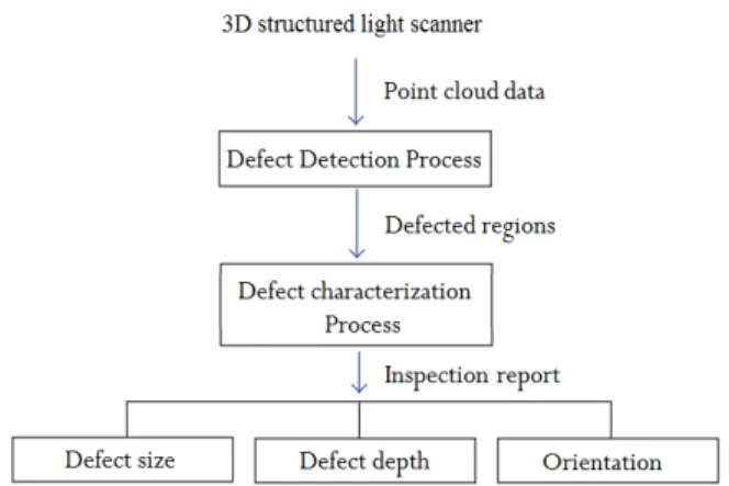
Fig.1illustrates all the steps of our approach. We use a personal computer for processing point clouds acquired from a structured light 3D scanner. First, a defect de-tection module identifies and localizes the presence of defects or deformations on the airplane exterior surface. Then, we analyse the status of all the defected regions and extract information about the defects size, depth and orientation. We termed this second phase as defect characterization process.
The 3D data processing program must ensure
robust-Fig. 1 Overview of proposed system architecture
ness for industrial applications. In other words, it must be able to detect di↵erent types of defects with di↵erent properties.
3.2 Data acquisition
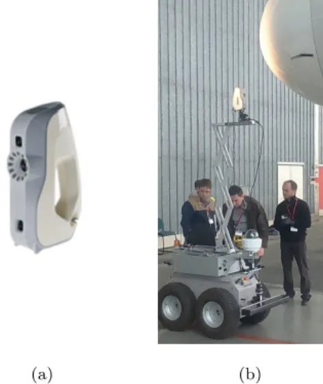
Our approach is applied to inspect the fuselage of real Airbus A320 airplane. The dataset is captured using a 3D scanner mounted on Air-Cobot (see Fig.2a and5b). The process is fully automatic and performs inspection of the body as the Air-Cobot moves following a pre-determined trajectory like Fig.2b. In order to test the
Fig. 2 (a) Air-Cobot and Airbus A320 airplane; (b) Illustra-tion of moving map of Air-Cobot
robustness of our approach, we collected data of vari-ous types of defects such as undesired dents or scratches under di↵erent light and weather conditions. Few exam-ples of our dataset are shown in Fig.3.
3.3 Defect detection process
In this section, we introduce the defect detection pro-cess as illustrated in Fig.4. The process is divided into
4 Igor Jovanˇcevi´c et al.
(a) (b)
(c) (d)
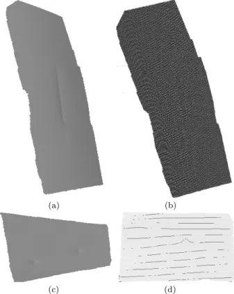
Fig. 3 (a) Point cloud of surface without defect; (b) point cloud with large and small dents (c) point cloud with small dents;(d) point cloud with a long scratch
five steps. First, 3D point cloud is acquired using a 3D scanner. Next, it is smoothed by Moving Least Squares (MLS) algorithm. Further, we calculate the normal and curvature information of each point in the point cloud. We employ Region-Growing for segmenting the point cloud into two sets of points: (1) defected regions and (2) non-defected regions. Finally, these two sets are ac-cordingly labeled for visualization.
Fig. 4 Overview of the detection phase
Step 1 ( data): With the advances of 3D scanning technologies, various types of 3D sensors have been de-veloped for acquiring 3D data of high quality. This tech-nology is very useful for material inspection and qual-ity control. It allows to collect a lot of 3D data about the object surface and its size. Di↵erent 3D scanners such as FARO Focus 3Dr, Trimbler, Artec Evar, or Handyscan 3Dr can be used for our work. After ana-lyzing the data quality of di↵erent types of scanner, we
decided to use Artec Eva 3D scanner (see Fig.5a). It scans quickly, in high resolution (0.5 mm) and accuracy (0.1 mm). Artec 3D scanner is also very versatile. It is recommended to keep the distance between the scanner and the object in the range 0.4 1m. The scanner has field of view up to 536⇥371mm (for furthest range) and frame rate of 16 frames per second. It should be noted, however, that the fundamental part of our system does not need to be changed if we want to use another type of 3D scanner.
(a) (b)
Fig. 5 (a) Artec Eva 3D scanner; (b) Air-Cobot with the scanner mounted on a pantograph
Step 2 (Pre-processing): Although the quality of 3D scanners has been improved greatly, we still get in-evitable measurement errors and outliers in point cloud. The goal of this step is to smooth and re-sample point cloud data. This pre-processing step is important be-cause it gives more accurate local information. We use Moving Least Squares (MLS) for smoothing the sur-face. MLS is a method of reconstructing a surface from a set of unorganized point data by higher order poly-nomial interpolations in the neighborhood of a fixed point. This technique was proposed by Lancaster and Salkauskas in 1981 [27] and developed by Levin [28,29]. We are approximating our cloud with a polynomial of second degree in Rn, since airplane fuselage is closest to
this type of surface. The mathematical model of MLS algorithm is described as follows:
Consider a function f : Rn 7! R and a set of points
S ={xi, fi|f(xi) = fi} where xi2 Rnand fi2 R. The
Moving Least Square approximation of the point xi is
the error functional: fM LS(xi) =
X
i
We achieve the weighted least-square error at bf where: b
f = min(fM LS(xi)) = min(k f(xi) fik)2⇥(k x xik)
In equation (1), the function ⇥ is called weighting func-tion. Authors have proposed di↵erent choices for this function. For example, in [29] the author used a Gaus-sian function: ⇥(d) = eh2d2. By applying the MLS
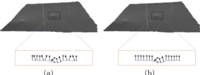
al-gorithm, we can remove the small errors and further estimate the intrinsic properties of the surface such as normal and curvature (see Fig.6).
(a) (b)
Fig. 6 Surface normal estimation on the: (a) original point cloud before resampling and (b) after resampling using Mov-ing Least Squares algorithm
Step 3 (Normals and Curvature Estimation): In 3D geometry, a surface normal at a point is a vec-tor that is perpendicular to the surface at that point. The surface normals are important information for un-derstanding the local properties of a geometric surface. Many di↵erent normal estimation techniques exist in
Fig. 7 Illustration of surface normals
the literature [24,8,31]. One of the simplest methods to estimate the normal of a point on the surface is based on estimating the normal of a plane tangent to the sur-face [41].
Given a point cloud PN, we consider the neighboring
points PKof a query point p
q. By using a least-square
plane fitting estimation algorithm as introduced in [47], we can determine the tangent plane S represented by a point x and a normal vector nx. For all the points
pi2 PK, the distance from pito the plane S is defined
as : di= (pi x)· nx S is a least-square plane if di= 0. If we set x as a centroid of PK: x = p = 1 K K X i=0 (pi)
in order to estimate nx, we need to analyze the
eigen-values j and eigenvectors vj (j = 0, 1, 2) of the 3⇥ 3
covariance matrix A formed by the points pi2 PK :
A = 1 K K X i=0 (pi p).(pi p)T (2)
The eigenvector v0corresponding to the smallest
eigen-value 0is the approximation of n [41].
Another surface property that we are using in de-fect detection is curvature. In computer graphics, there are many ways to define the curvature of a surface at a point such as Gaussian curvature (K = k1k2), or
Mean Curvature (H = k1+ k2
2 ) [10] where k1 and k2 are the principal curvatures of the surface. In the lit-erature, these methods are widely used for calculating curvature information [39]. Some other techniques have been proposed by the authors in [59,25]. The above approaches are accurate but very sensitive to noise and unable to estimate the curvature from a set of points di-rectly (mesh representation required). We estimate the curvature information at a specific point by analysing the eigenvalues of covariance matrix defined in equation
2.
The curvature value of a point Pj is estimated as:
c{Pj} =
0
0+ 1+ 2
(3) where 0 = min ( j=0,1,2) [38].
To resume, we estimate surface normals and curva-ture of each point in the cloud. This information is used in the next step.
Step 4 (Segmentation): In order to detect the damaged regions on airplane exterior surface, we need to segment the 3D points cloud data into regions that are homogeneous in terms of calculated surface char-acteristics, more specifically normal vector angles and curvature di↵erences. By this way, we can divide orig-inal point cloud into two principal parts: damaged re-gions and non-damaged rere-gions. The objective of this step is to partition a point cloud into sub-point clouds based on normal and curvature information which are calculated in step 3.
6 Igor Jovanˇcevi´c et al. Let P represent the entire input point cloud, the
region-based segmentation divides P into n sub-point clouds R1, R2, R3, ...Ri..., Rn such that:
(1) n S i=1 Ri= P (2) Riis connected region (i = 1, n )
(3) Ri\ Rj=↵ for all i and j, i 6= j
(4) LP (Ri) = True for i = 1, n
(5) LP (Ri[ Ri) = False for any adjacent regions Ri
and Rj
LP (Ri) is a logical predicate defined on the points p2
Ri. Condition (4) indicates that the di↵erences in
sur-face properties (normal and curvature in our case) in a segmented region must be below certain threshold. Condition (5) regulates the di↵erence between adjacent regions which should be above the threshold. The algo-rithm starts with random points (Pseeds) representing
distinct regions and grow them until they cover the en-tire cloud. For region growing, we need a rule for check-ing the homogeneity of a region after each growth step. In this paper, we have used surface normals and curva-tures to merge the points that are close enough in terms of the smoothness constraint. The picked point is added to the set called seeds. In each iteration a seed point is chosen from the set of unlabeled points. Seed point is always selected as a point with the lowest curvature in the current set of unlabeled points. For every seed point, the algorithm finds neighboring points (30 in our case). Every neighbor is tested for the angle between its normal and normal of the current seed point. If the an-gle is less than a threshold value, then current point is added to the current region. Further, every neighbour is tested for the curvature value. If the curvature is less than threshold value cth, then the point is added to the
seeds [42]. The criteria is shown in Eq.4:
arccos(n, nk) ↵th, (4)
where n and nk are normals of the seed point p and
current tested point pk, respectively.
By this way, the output of this algorithm is the set of clusters, where each cluster is a set of points that are considered to be a part of the same smooth surface. We finish by obtaining one vast cluster which is consid-ered background and a lot of small clusters only in the defected regions. Admittedly, we obtained several clus-ters within the same defect, but we solve this by simply merging adjacent clusters. Our defects are never close to each other so this merging step is safe to be done.
The segmentation algorithm presented in step 4 can be described as following:
Algorithm 1: Point cloud segmentation based on surface normal and curvature
Input: Point cloud P = p1, p2...., pN; Point normals N ; Point curvatures C ; Angle threshold ↵th; Curvature threshold cth; Neighbour finding function F (·)
Process:
1: Region list{R} ↵
2: Available points list{L} {1..|P |} 3: While{L} is not empty do
4: Current region{Rc} ↵ 5: Current seeds{Sc} ↵
6: Point with minimum curvature in{L} = Pmin 7: {Sc} {Sc} [ Pmin
8: {Rc} {Rc} [ Pmin 9: {L} {L} \ Pmin 10: For i = 0 to size ({Sc}) do
11: Find nearest neighbors of current seed point {Bc} F (Sc{i})
12: For j = 0 to size ({Bc}) do
13: Current neighbor point Pj Bc{j} 14: If Pj2 L and
arccos ( (N{Sc{i}}, N{Sc{j}}) ) < ↵ththen 15: {Rc} {Rc}SPj 16: {L} {L} \ Pj 17: If c{Pj} < cththen 18: {Sc} {Sc} [ Pj 19: End if 20: End if 21: End for 22: End for
23: Global segment list{R} {R}S{Rc} 24: End while
25: Return the global segment list{R}
Outputs: a set of homogeneous regions R ={Ri}.
Step 5 (Labeling): The previous algorithm allows determining the regions which contain points that be-long to defects. The defects are labeled by the algorithm in order to show them on the original point cloud. The resulting labeling is shown in red color as in Fig.8:
3.4 Defect characterization process
Next step is to characterize the defects by estimating their size and depth. For that, we use the result of the defect detection process.
(a) (b)
(c)
Fig. 8 (a) Part of the fuselage; (b) Acquired point cloud (visualized with MeshLab).; (c) The detected defects on the original mesh are shown in red color
The purpose of this process is to extract and show the most important information about each detected defect. In our study, we propose an approach that allows estimating three main information about a defect, in-cluding size (bounding box), the maximum depth, and the principal orientation of a defect. Orientation is use-ful in the case of scratch-like defects (ex. Fig.12a).
Our global approach can be viewed as a 4-step pro-cess (Fig.9): (1) projection of the 3D point cloud onto the fronto-parallel 2D image plane (2) data prepara-tion, (3) reconstrucprepara-tion, and (4) extracting information about the defects. Further on we will explain each of the steps.
Fig. 9 Global approach of characterization process
3.4.1 Step C1 : 3D/2D projection
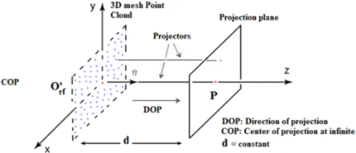
We are reducing our problem from 3D to 2D by pro-jecting our 3D cloud onto the fronto-parallel 2D image
plane placed on a certain distance from the cloud. We do this in order to reduce computational cost and also to facilitate operations such as neighbors search in char-acterization phase. We do not lose information because our clouds are close to planes. After this process, each 3D point can be referenced by its 2D projection (pixel). Planar geometric projection is mapping 3D points of a 3D object to a two-dimensional plane called pro-jection plane. It is done by passing lines (projectors) through 3D points and calculating their intersections with projection plane. Depending on the center of pro-jection (COP), there are two principal kinds of projec-tion: parallel and perspective projection [6]. When the COP is placed on a finite distance from the projection plane, perspective projection is obtained. In the case of parallel projection, the COP is considered to be at infin-ity and projectors are parallel. Orthographic projection is a subclass of parallel projection which is obtained when the projectors are orthogonal to the projection plane. If the scale is introduced in a uniform manner, it is said that scaled orthographic projection is performed. Scale is added in a way that the whole object is uni-formly decreased/increased after being projected. This type of projection is also called weak perspective pro-jection. It assumes that relative depths of object points are negligible compared to the average distance between the object and COP.
In our work, we are performing a scaled orthographic projection of our point cloud. The projection plane is placed on a certain distance d from the cloud and ori-ented approximately parallel to the cloud. The point cloud points are represented by their (x, y, z) coordi-nates in scanner reference system. We are expressing these points in the new coordinate system which en-ables the projection to be straightforward. This new coordinate system is placed in the mean point of the cloud with mean normal of the cloud as its z axis (O0rf in Fig.11). Finally, this system is translated for length d along its z axis. The process consists of 3 steps.
Step C1.1 (Find the mean normal of the point cloud)
The notion of centroid can apply to vectors. Let V be a set of N normal vectors in all the points of the cloud:
V ={n1, n2...nN} with ni= [xni, yni, zni]
T
The mean normal is calculated as: n = 1 N N P i=1 ni= (xn, yn, zn)
8 Igor Jovanˇcevi´c et al. bn = n knk= xn knk, yn knk, zn knk ! whereknk =px2 n+ yn2+ zn2 .
Step C1.2 (Calculate the rotation and trans-formation matrix)
When the point cloud is created, it is defined in the reference system of the scanner Orf. We define a new
reference system O0rf in which zO0
rf = bn where zO 0 rf
is a unit vector along z axis of the new reference sys-tem O0rf. The origin of O0rf is unchanged. Further, we find the rotation matrix which aligns two unit vectors zOrf = [0, 0, 1] and zOrf0 =bn. This task can be solved
as follows.
It should be noted that the 3D rotation which aligns these two vectors is actually a 2D rotation in a plane with normal zOrf⇥ bn by an angle ⇥ between these two
vectors: R = 2 6 4 cos ✓ sin ✓ 0 sin ✓ cos ✓ 0 0 0 1 3 7 5
Since cos ✓ = zOrf · bn and sin ✓ = kzOrf ⇥ bnk, we
further obtain: R = 2 6 4 zOrf · bn kzOrf ⇥ bnk 0 kzOrf⇥ bnk zOrf · bn 0 0 0 1 3 7 5 = 2 6 4 x1y10 x2y20 0 0 1 3 7 5 With R we defined a pure z-rotation which should be performed in the reference frame whose axes are (zOrf, b n (zOrf·bn)zOrf kbn (zOrf·bn)zOrfk, zOrf⇥ b n (zOrf·bn)zOrf
kbn (zOrf·bn)zOrfk). It can
be easily verified that this is an orthonormal basis. If we denote zOrf with A andbn with B, the axes are
illus-trated in Fig.10whereBP
Ais the projection of vector
B onto the vector A.
Fig. 10 Constructing the new orthonormal base. Thick blue vectors denote x and y vectors of new reference frame (not yet normalized).
Matrix for changing basis is then:
C = (zOrf,
bn (zOrf· bn)zOrf
kbn (zOrf· bn)zOrfk
, zOrf⇥ bn)
1.
Further, we multiply all the cloud points with C 1RC.
With C we change the basis, with R we perform the ro-tation in the new basis and C 1brings the coordinates
back to the original basis. After this operation we have our cloud approximately aligned with xy plane of the original frame and approximately perpendicular to the z axis of the same frame.
Step C1.3 (Orthographic projection and trans-lation in image plane)
Once the cloud is rotated, orthographic projection on the xy plane means just keeping x and y coordinates of each point.
u = x; v = y
Some of these values can be negative. In that case, we are translating all the 2D values in order to obtain positive pixel values and finally create an image. Let pneg = (upneg, vpneg) be the most negative 2D point in
the set of projected points. We are translating all the points as follows:
ui= ui+kupnegk
vi= vi+kvpnegk
The projection process is illustrated in Fig.11. Ex-amples of two point clouds and their projections are shown in Fig.12. The projection is better visible in the Fig.13a.
Fig. 11 Orthographic projection from 3D point cloud to 2D plane
As the last step in C1 phase, in the image space, we perform resampling of projected pixels (Fig. 13). Af-ter projection, pixels are scatAf-tered (Fig.13a). Resam-pling is done in order to have regular grid of projected
(a) (b)
(c) (d)
Fig. 12 (a),(c) 3D mesh of original point cloud; (b),(d) 2D image after projecting
points. Regular grid, shown in Fig.13b, makes neigh-bors search faster by directly addressing neighboring pixels with their image coordinates instead of search-ing among scattered points.
(a) (b)
Fig. 13 (a) scattered pixels after projection (b) regular grid after resampling
The same as the whole input point cloud, the de-fected regions are separately projected onto another 2D image. An example is shown in Fig.14. Note that these images have the same size as the projection of the orig-inal point cloud.
3.4.2 Step C2 : Data preparation
The second step of the characterization process is the preparation of data. There are three di↵erent types of data which are essential for this process: (1) the orig-inal point cloud, (2) identified points belonging to the defect-regions, and (3) the polygon surrounding each defect. The point cloud and all the defect-regions are available from Sec.3.3.
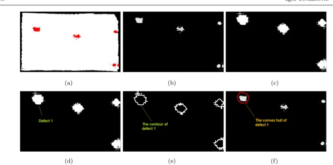
In order to obtain the surrounding polygon of a defect, we start from the binary image with all projected defect points after the projection process (Fig.14b). Note that the input data can contain one or several defects. For the defects located in close proximity, we group these defects into one by using the mathematical morphology operation called dilation [14]. This operator also allows to enlarge the boundaries of defect-regions (Fig.14c).
After dilating the defect-regions, we identify con-nected components [15] on binary image (see Fig.14d). Each of the connected components corresponds to a damage. Further, contours are extracted for each de-fect (see Fig.14e). The convex hull [16] of the defect is then determined as in Fig.14f and taken as the polygon surrounding the points which belong to the defect.
3.4.3 Step C3 : Reconstruction
Our main idea in this section is to reconstruct the ideal surface of the 3D data. This ideal surface is further used as a reference to extract the information about the status of defect by comparing the variance between the z-coordinate value of each point in the ideal surface and the corresponding point in the original data. The concept is illustrated in Fig.15.
In order to reconstruct the ideal surface of the 3D data, we use a method called Weighted Least Squares (WLS) [33]. We are fitting a quadratic bivariate poly-nomial f (u, v) : R2 ! R to a set of cloud points which
are out of the polygonal defect area. We justify this by the shape of the airplane fuselage which is close to the quadratic surface.
We start with a set of N points (ui, vi)2 R2 with
their z-values zi 2 R. All these values are obtained in
the projection phase. We search for a globally-defined function f (u, v) = z, that best approximates the sam-ples. The goal is to generate this function such that the distance between the scalar data values zi and the
function evaluated at the points f (ui, vi) is as small as
possible. This is written as: min =
N
X
i=1
10 Igor Jovanˇcevi´c et al.
(a) (b) (c)
(d) (e) (f)
Fig. 14 (a) Labeled defects after detection; (b) Binary image after projecting defects onto the plane; (c) Defect regions after dilation; (d)Identifying each connected component as one defect; (e) Contours of the enlarged defects; and (f) Convex hull of each defect
Fig. 15 An illustration of the approach for calculating defect depth
where (u, v) is a fixed point, for ex. center of mass of the defect region. We can find many choices for the weighting function ✓(d) in the literature such as a Gaus-sian [29] or the Wendland function [55]. It is a function which is favorizing the points which are in the proxim-ity of the defect, while assigning lower weights to the points far away from the fixed point (u, v).
3.4.4 Step C4 : Extracting information about the defects
The lowest point
For each point in a defect region, we estimate the values z(pi) = zP (ideal) z(pi). Here, pi is a point
belonging to a defect region. We do not consider pi as
a defect point if z(pi) is lower than a predefined
threshold. The lowest point of the defect is determined by max{ z(pi)} among all the points from that
de-fect region. The sign of z(pi) determines if defect is a
dent or a protrusion. A dent is detected when z(pi)
is positive and a protrusion is detected when z(pi) is
negative.
The dimension and orientation of defect
In order to show the size and the orientation of the defect, we construct an oriented bounding-box (OBB) [17]. We rely on Principal Component Analysis (PCA) [21]. Let X be a finite set of N points in R2. Our
prob-lem consists of finding a rectangle of minimal area en-closing X.
(a) (b)
Fig. 16 Illustration of the PCA bounding-box of a set of points X2 R2
The main idea of PCA is to reduce the dimensional-ity of a data set based on the most significant directions or principal components. For performing a PCA on X, we compute the the eigenvectors of its covariance ma-trix and choose them as axes of the orthonormal frame e⇠ (see Fig.16b). The first axis of e⇠ is the direction of
largest variance and the second axis is the direction of smallest variance [9]. In our case, given a finite set of points in the defect-regions, we first calculate the center of mass of the defect and then apply the PCA algorithm for determining e⇠. We continue by searching the end
points along two axes of e⇠. These points allow us to
draw an oriented bounding-box of the defect as we can see for ex. in Fig.17c .
4 Experiments and discussion
The proposed method has been tested on 15 point clouds, both with and without defective regions. The items which have been used to test and illustrate our ap-proach are: radome, static port with its surrounding area and some parts of the fuselage. This set is con-sidered representative since the radome (airplane nose) has a significant curvature (Fig.22a) while static port (Fig.22c) and fuselage (Fig. 20a) are the surfaces rel-atively flat. We obtained promising results which will further be illustrated. We acquired point clouds using the Artec Eva 3D scanner at Air France Industries tar-mac and Airbus hangar in di↵erent lighting conditions. We acquired scans of aircraft surface with multiple de-fects. The same parameters of the detection algorithm are used for most of the input clouds. The scanner was placed 60 100 cm from the surface. Specifically, we choose angle threshold ↵th = 0.25 and the curvature
threshold cth= 0.3. The original point clouds, detected
defects and the corresponding characterization results for each defect are shown in Fig.17, Fig. 18, Fig. 19, Fig.20, Fig.21, and Fig.22.
The parameters we use in our algorithm play an im-portant role in detecting the defects. The most impor-tant one is the angle threshold ↵th. In our experiments,
we have used ↵th in the range {0.2 ⇠ 1} degrees. In
most cases, we have set ↵th= 0.25. When we reduced
the value of angle threshold ↵th, the sensitivity of the
algorithm increased. Fig.23shows the influence of the value ↵thon the area of detected defect.
For curvature threshold cth, we test the algorithm
on our dataset and we set it to cth = 0.3. This study
also indicates that the performance of the program is influenced by various factors, as scanning mode, scan-ning distance, density of point cloud and dimensions of the defects (depth, area).
(a) (b)
(c) (d)
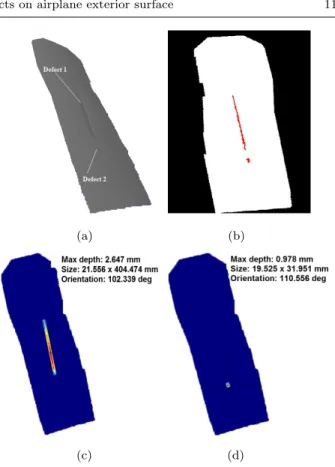
Fig. 17 Scratch on fuselage. (a) Original point cloud; (b) Defects detected; (c) Information about defect 1; (d) Infor-mation about defect 2
12 Igor Jovanˇcevi´c et al. Defect 1 Defect 4 Defect 2 Defect 3 (a) (b) Defect 1 Max depth: 1.803 mm Size: 21.244 x 44.245 mm Orientation: 180 deg Defect 2 Max depth: 2.397 mm Size: 27.255 x 42.269 mm Orientation: 169.695 deg (c) (d) Defect 3 Max depth: 0.852 mm Size: 16.681 x 21.384 mm Orientation: 239.036 deg Defect 4 Max depth: 0.835 mm Size: 11.242 x 14.781 mm Orientation: 194.036 deg (e) (f)
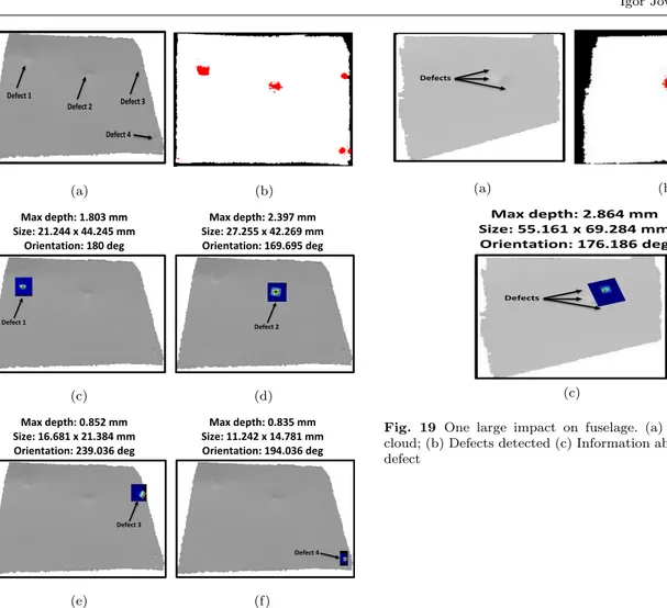
Fig. 18 Four impacts on fuselage. (a) Original point cloud; (b) Defects detected; (c) Information about defect 1; (d) In-formation about defect 2; (e) InIn-formation about defect 3; (f) Information about defect 4
Defects (a) (b) Defects Max depth: 2.864 mm Size: 55.161 x 69.284 mm Orientation: 176.186 deg (c)
Fig. 19 One large impact on fuselage. (a) Original point cloud; (b) Defects detected (c) Information about the largest defect
(a) (b)
(c) (d)
(e) (f)
Fig. 20 Four defects on fuselage. (a) Original point cloud; (b) Defects detected; (c) Information about defect 1; (d) In-formation about defect 2; (e) InIn-formation about defect 3; (f) Information about defect 4
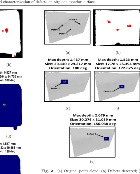
Defect 1 Defect 2 Defect 3 (a) (b) Defect 1 Max depth: 1.437 mm Size: 20.140 x 29.217 mm Orientation: 180 deg Defect 2 Max depth: 1.523 mm Size: 17.78 x 25.394 mm Orientation: 172.875 deg (c) (d) Defect 3 Max depth: 2.079 mm Size: 30.276 x 31.039 mm Orientation: 156.038 deg (e)
Fig. 21 (a) Original point cloud; (b) Defects detected; (c) Information about defect 1; (d) Information about defect 2; (e) Information about defect 3
(a) (b)
(c) (d)
Fig. 22 Examples of point clouds without defects: (a) Radome; (c) Static port ; (b) and (d) Detection result
14 Igor Jovanˇcevi´c et al.
(↵th= 0.2) (↵th= 0.25)
(↵th= 0.3) (↵th= 0.35)
(↵th= 0.4) (↵th= 0.45)
(↵th= 0.5) (↵th= 1.0)
Fig. 23 The influence of the value ↵thon the detection re-sults
4.1 Evaluation using dial gauge ground truth
In practice, the fuselage inspection is done manually by a quality manager who first examines the surface using a low angle light in order to detect defects. Next, the zone around the detected defect is demarcated with a marker pen. The zone is further examined using a dial gauge, also named dial indicator. This instrument is shown in Fig.24a and its functioning principle is illus-trated in Fig.24b. The probe is traversing the defective area until surface contact occurs.
Obvious drawback of this method is that it depends on the expertise and mood of the person operating the equipment. Another flaw appears in the case of larger defects, such as those in Fig.18c and Fig.18d. Having a measuring stand with a fixed standardized diameter, the gauge can dive into the defect and report a lower depth than the real one (Fig.25). An advantage of our method is that it can characterize defects of any size.
(a) (b)
Fig. 24 (a) AIRBUS standardized dial gauge; (b) Illustra-tion of dial gauge funcIllustra-tioning
Fig. 25 Imprecision in measuring depth in the case of large defects. Red: depth measured by dial gauge; Blue: real depth.
(a) (b) Defect 5
Max depth: 0.271 mm
Size: 3.997 x 1.628 mm
Orientation: 180 deg
Defect 6Max depth: 0.474 mm
Size: 3.453 x 5.974 mm
Orientation: 180 deg
(c) (d)Fig. 26 (a) Part of the fuselage; (b) The detected defects are shown in red color; (c) Information about defect 5 (Dial gauge max depth: 0.31mm); (d) Information about defect 6 (Dial gauge max depth: 0.48mm)
In the case of small defects, we compared our method with the result obtained by AIRBUS experts using their standardized dial gauge (diameter of the measuring stand 34mm) shown in Fig. 24a. Fig. 26a shows the same part of the fuselage as the one in Fig.8, with indicated two additional defects (5 and 6), hardly visible to an eye. For detecting these shallow defects, ↵th had to be
decreased. For this reason, sensitivity of our detection phase increased. Consequently, we produced some false detections as well (Fig.26b).
Fig. 26c and 26d show that the estimated maxi-mal depths obtained by our approach are 0.27mm and 0.47mm while standardized AIRBUS dial gauge results are 0.31mm and 0.48mm respectively. The average dis-crepancy is around 8%.
For the reason of small diameter measuring stand, we could not obtain accurate results with the same dial gauge for neither of the defects larger than 34mm. Therefore, we carried on the measuring in laboratory conditions. Our setup is shown in Fig.27. Part of the fuselage was fixed on XY mobile table used for precise cutting of composite materials. The part was placed as parallel as possible with the table in order to min-imize inclination. Dial gauge (with 0.01mm gradua-tions) without limiting measuring stand was fixed by using magnetic base. Rectangular grid was drawn around each defect and the part was slowly moved along X and
16 Igor Jovanˇcevi´c et al. Y axis of the table. In all the intersections points of the
grid, the depth is measured by the dial gauge.
(a) (b)
Fig. 27 Measuring the depth of defects with Dial gauge; (a) Measuring setup; (b) Dial gauge
This way we obtained 10cm long profile lines. Val-ues read along middle lines are shown in Fig. 28 to-gether with our results. In order to take into account possible inclination of the fuselage part, the depth is obtained by measuring the di↵erence between the low-est point (black squares in Fig. 28) and the line ob-tained as average of end values on the profile (red lines in Fig.28). The discrepancies between the Dial gauge measurements and our measured values (Fig.18 c and d) are e =|1.8 1.7| = 0.1mm (6%) and e = |2.44 2.4| = 0.04mm (2%). The values obtained by the three mea-surement methods are given in Table1. This table con-firms our doubt that, in case of large defects (defects 1 and 2), AIRBUS gauge depth values are underesti-mated due to the measuring stand issue. The other tests that have been carried out so far on large defects have shown that the discrepancy is on average 5% and al-ways below 10%. As per defects 3 and 4 from the same cloud (Fig. 18 e and f), it was impossible to measure them with dial gauge because those are two holes. How-ever, having similar values for these two defects ( 0.85 and 0.84) is coherent since they are two identical screw holes produced in the manufacturing phase.
(a) (b)
Fig. 28 (a) Profile for defect 1 (Fig. 18c); (b) Profile for defect 2 (Fig.18d)
It should be noted that dial gauge method does not take into account the curvature of the fuselage which can a↵ect the characterization process of defects above certain size. Contrary, with the ideal surface
reconstruc-tion explained in Sec.3.4.3, our approach considers this aspect of the problem.
Table 1 Maximal depth of large defects shown in Fig.18 Our method Dial gauge AIRBUS dial gauge
Defect 1 1.80 1.70 1.42
Defect 2 2.40 2.44 1.73
4.2 Execution time
Execution time of the whole process is not easily quan-tifiable because it depends on density and size of the cloud (number of points) as well as on the number of defects. It should be noted that characterization process is performed for each detected defect sequentially. Also, in our process we are converting the input cloud from the scanner format to the format suitable for process-ing, which also takes time. However the total processing time which varies between 20s and 120s on our dataset, is acceptable for our application since the 3D inspec-tion is planned to be done during more detailed and longer check, usually in the hangar. These values were obtained by testing non-optimized code on the PC with: 2.4 GHz Core(TM) i7 CPU, 8GB RAM with Microsoft Visual Studio 2013. The method was developed in C++ with the support of Point Cloud Library v.1.7.0 cite [42] and OpenCV v.3.0. library [5]. Approximately for a cloud with 30000 points, detection phase takes around 8 9s while characterization step takes 2 3s for each defect. Our time rises up to 120s because some of our clouds contain redundant information, caused by the longer exposure time. It is experimentally established that this scanning mode is not useful and ”one shot” scanning mode is recommended. Typical cloud obtained with ”one shot” scanning mode contains 30000 points. Therefore typical processing time is 20s, if we assume that typical number of detected defects is 3 5.
5 Conclusions
In this paper, an original framework for the detection and characterization of defects in point cloud data has been presented. Proposed methodology is divided into two main processes. The first process is the defects de-tection. In this process, the Point Cloud is segmented to identify the defect regions and non-defect regions. A computer vision algorithm which is able to detect various undesired deformations on airplane surface was
developed using Region-Growing method with the local information about surface including points normal and curvature. In the next process, we developed a tech-nique for characterizing the defects. This techtech-nique al-lows us to provide information about each defect such as the size, the depth and the orientation. Experiments are conducted on real data captured by 3D scanner on the fuselage of Airbus A320 airplane. This is a set of clouds encompassing various characteristics. The experimen-tal results demonstrate that our approach is scalable, e↵ective and robust to clouds with noise and can de-tect di↵erent types of deformation such as protrusions, dents or scratches. In addition, the proposed processes work completely automatically. Finally, a limitation of our approach is processing-time. In the future, we plan to reduce program execution time by optimizing our code. Thus, we believe that our results are promising for application in an inspection system. Not only lim-ited to the context of airplane surface inspection, our approach can be applied in wide range of industrial ap-plications. Our approach is also limited to plane-like surfaces. Strongly curved surfaces, such as wings and engine cowling, cause our characterization approach to fail. We propose cloud fitting to the available Computer Aided Design model of the airplane, in order to calcu-late ideal surface more precisely.
Acknowledgements This work is part of the AIR-COBOT project (http://aircobot.akka.eu) approved by the Aerospace Valley world competitiveness cluster. The authors would like to thank the French Government for the financial support via the Single Inter-Ministry Fund (FUI). The partners of the AIR-COBOT project (AKKA TECHNOLOGIES, Airbus Group, ARMINES, 2MoRO Solutions, M3 SYSTEMS and STERELA) are also acknowledged for their support. Nicolas Simonot and Patrick Metayer from AIRBUS/NDT are also acknowledged for their help in providing dial gauge measure-ments.
References
1. Benhabiles, H., Lavou´e, G., Vandeborre, J., Daoudi, M.: Learning boundary edges for 3d mesh segmentation. In: Computer Graphics Forum, vol. 30, pp. 2170–2182. Wiley Online Library (2011)
2. Besl, P.J., Jain, R.C.: Segmentation through variable-order surface fitting. Pattern Analysis and Machine In-telligence, IEEE Transactions on 10(2), 167–192 (1988) 3. Bhanu, B., Lee, S., Ho, C., Henderson, T.: Range data
processing: Representation of surfaces by edges. Univer-sity of Utah, Department of Computer Science (1985) 4. Borsu, V., Yogeswaran, A., Payeur, P.: Automated
sur-face deformations detection and marking on automotive body panels. In: Automation Science and Engineering (CASE), 2010 IEEE Conference on, pp. 551–556. IEEE (2010)
5. Bradski, G.: Dr. Dobb’s Journal of Software Tools
6. Carlbom, I., Paciorek, J.: Planar geometric projections and viewing transformations. ACM Computing Surveys (CSUR) 10(4), 465–502 (1978)
7. Deng, H., Zhang, W., Mortensen, E., Dietterich, T., Shapiro, L.: Principal curvature-based region detector for object recognition. In: Computer Vision and Pattern Recognition, 2007. CVPR’07. IEEE Conference on, p. 18. IEEE (2007)
8. Dey, T.K., Li, G., Sun, J.: Normal estimation for point clouds: A comparison study for a voronoi based method. In: Pointbased graphics, 2005. Eurograph-ics/IEEE VGTC symposium proceedings, pp. 39–46. IEEE (2005)
9. Dimitrov, D., Knauer, C., Kriegel, K., Rote, G.: On the bounding boxes obtained by principal component anal-ysis. In: 22nd European Workshop on Computational Geometry, pp. 193–196. Citeseer (2006)
10. Dyn, N., Hormann, K., Kim, S., Levin, D.: Optimizing 3d triangulations using discrete curvature analysis. Mathe-matical methods for curves and surfaces 28(5), 135–146 (2001)
11. Filin, S.: Surface clustering from airborne laser scanning data. International Archives of Photogrammetry Remote Sensing and Spatial Information Sciences 34(3/A), 119– 124 (2002)
12. Fua, P., Sander, P.: Segmenting unstructured 3d points into surfaces. In: Computer Vision - ECCV’92, pp. 676– 680. Springer (1992)
13. Golovinskiy, A., Funkhouser, T.: Randomized cuts for 3d mesh analysis. ACM transactions on graphics (TOG) 27(5), 145 (2008)
14. Gonzalez, R.C., Woods, R.E.: Digital image processing. Prentice Hall, Third Edition, pp. 669-671 (2002) 15. Gonzalez, R.C., Woods, R.E.: Digital image processing.
Prentice Hall, Third Edition, pp. 667-669 (2002) 16. Gonzalez, R.C., Woods, R.E.: Digital image processing.
Prentice Hall, Third Edition, pp. 655-657 (2002) 17. Gottschalk, S., Lin, M.C., Manocha, D.: Obbtree: A
hi-erarchical structure for rapid interference detection. In: Proceedings of the 23rd annual conference on Computer graphics and interactive techniques, pp. 171–180. ACM (1996)
18. Haddad, N.A.: From ground surveying to 3d laser scan-ner: A review of techniques used for spatial documen-tation of historic sites. Journal of King Saud Universi-tyEngineering Sciences 23(2), 109–118 (2011)
19. Hoover, A., JeanBaptiste, G., Jiang, X., Flynn, P.J., Bunke, H., Goldgof, D.B., Bowyer, K., Eggert, D.W., Fitzgibbon, A., Fisher, R.B.: An experimental compar-ison of range image segmentation algorithms. Pattern Analysis and Machine Intelligence, IEEE Transactions on 18(7), 673–689 (1996)
20. Jin, H., Yezzi, A.J., Soatto, S.: Region-based segmenta-tion on evolving surfaces with applicasegmenta-tion to 3d recon-struction of shape and piecewise constant radiance. In: Computer Vision - ECCV 2004, pp. 114–125. Springer (2004)
21. Jolli↵e, I.: Principal component analysis. Wiley Online Library (2002)
22. Katz, S., Tal, A.: Hierarchical mesh decomposition using fuzzy clustering and cuts, vol. 22. ACM (2003)
23. Khan, W.: Image segmentation techniques: A survey. Journal of Image and Graphics 1(4), 166–170 (2013) 24. Klasing, K., Altho↵, D., Wollherr, D., Buss, M.:
Com-parison of surface normal estimation methods for range sensing applications. In: Robotics and Automation, 2009. ICRA’09. IEEE International Conference on, pp. 3206– 3211. IEEE (2009)
18 Igor Jovanˇcevi´c et al. 25. Koenderink, J.J., van Doorn, A.J.: Surface shape and
cur-vature scales. Image and vision computing 10(8), 557– 564 (1992)
26. K¨oster, K., Spann, M.: Mir: an approach to robust clustering-application to range image segmentation. Pat-tern Analysis and Machine Intelligence, IEEE Transac-tions on 22(5), 430–444 (2000)
27. Lancaster, P., Salkauskas, K.: Surfaces generated by mov-ing least squares methods. Mathematics of computation 37(155), 141–158 (1981)
28. Levin, D.: The approximation power of moving leasts-quares. Mathematics of Computation of the American Mathematical Society 67(224), 1517–1531 (1998) 29. Levin, D.: Mesh-independent surface interpolation. In:
Geometric modeling for scientific visualization, pp. 37– 49. Springer (2004)
30. Marani, R., Roselli, G., Nitti, M., Cicirelli, G., D’Orazio, T., Stella, E.: A 3d vision system for high resolution sur-face reconstruction. In: Sensing Technology (ICST), 2013 Seventh International Conference on, pp. 157–162. IEEE (2013)
31. Mitra, N.J., Nguyen, A.: Estimating surface normals in noisy point cloud data. In: Proceedings of the nineteenth annual symposium on Computational geometry, pp. 322– 328. ACM (2003)
32. Mumtaz, R., Mumtaz, M., Mansoor, A.B., Masood, H.: Computer aided visual inspection of aircraft surfaces. In-ternational Journal of Image Processing (IJIP) 6(1), 38 (2012)
33. Nealen, A.: An as-short-as-possible introduction to the least squares, weighted least squares and moving least squares methods for scattered data approximation and interpolation. URL: http://www. nealen. com/projects 130, 150 (2004)
34. Nguyen, A., Le, B.: 3d point cloud segmentation: A sur-vey. In: Robotics, Automation and Mechatronics (RAM), 2013 6th IEEE Conference on, pp. 225–230. IEEE (2013) 35. Nurunnabi, A., Belton, D., West, G.: Robust segmenta-tion in laser scanning 3d point cloud data. In: Digital Im-age Computing Techniques and Applications (DICTA), 2012 International Conference on, p. 18. IEEE (2012) 36. Nurunnabi, A., West, G., Belton, D.: Robust methods for
feature extraction from mobile laser scanning 3d point clouds
37. Pauling, F., Bosse, M., Zlot, R.: Automatic segmentation of 3d laser point clouds by ellipsoidal region growing. In: Australasian Conference on Robotics and Automation (ACRA) (2009)
38. Pauly, M., Gross, M., Kobbelt, L.P.: Efficient simplifica-tion of point-sampled surfaces. In: Proceedings of the conference on Visualization’02, pp. 163–170. IEEE Com-puter Society (2002)
39. Peng, J., Li, Q., Kuo, C.J., Zhou, M.: Estimating gaus-sian curvatures from 3d meshes. In: Electronic Imaging 2003, pp. 270–280. International Society for Optics and Photonics (2003)
40. Rabbani, T., Van Den Heuvel, F., Vosselmann, G.: Seg-mentation of point clouds using smoothness constraint. International Archives of Photogrammetry, Remote Sens-ing and Spatial Information Sciences 36(5), 248–253 (2006)
41. Rusu, R.B.: Semantic 3d object maps for everyday ma-nipulation in human living environments. Ph.D. thesis, Technische Universit¨at M¨unchen (2009)
42. Rusu, R.B., Cousins, S.: 3D is here: Point Cloud Library (PCL). In: IEEE International Conference on Robotics and Automation (ICRA). Shanghai, China (2011)
43. Rusu, R.B., Marton, Z.C., Blodow, N., Dolha, M., Beetz, M.: Towards 3d point cloud based object maps for house-hold environments. Robotics and Autonomous Systems 56(11), 927–941 (2008)
44. Sappa, A.D., Devy, M.: Fast range image segmentation by an edge detection strategy. In: 3D Digital Imaging and Modeling, 2001. Proceedings. Third International Con-ference on, pp. 292–299. IEEE (2001)
45. Schnabel, R., Wahl, R., Klein, R.: Efficient ransac for point cloud shape detection. In: Computer graphics fo-rum, vol. 26, pp. 214–226. Wiley Online Library (2007) 46. Seher, C., Siegel, M., Kaufman, W.M.: Automation tools
for nondestructive inspection of aircraft: Promise of tech-nology transfer from the civilian to the military sector. In: Fourth Annual IEEE DualUse Technologies and Ap-plications Conference (1994)
47. Shakarji, C.M., et al.: Leasts-quares fitting algorithms of the nist algorithm testing system. Journal of ResearchNa-tional Institute of Standards and Technology 103, 633– 641 (1998)
48. Siegel, M., Gunatilake, P.: Remote inspection technolo-gies for aircraft skin inspection. In: Proceedings of the 1997 IEEE Workshop on Emergent Technologies and Vir-tual Systems for Instrumentation and Measurement, Ni-agara Falls, CANADA, pp. 79–78 (1997)
49. Siegel, M., Gunatilake, P., Podnar, G.: Robotic assistants for aircraft inspectors. Industrial Robot: An International Journal 25(6), 389–400 (1998)
50. Simari, P., Nowrouzezahrai, D., Kalogerakis, E., Singh, K.: Multi-objective shape segmentation and labeling. In: Computer Graphics Forum, vol. 28, pp. 1415–1425. Wiley Online Library (2009)
51. Strom, J., Richardson, A., Olson, E.: Graph-based seg-mentation for colored 3d laser point clouds. In: Intelligent Robots and Systems (IROS), 2010 IEEE/RSJ Interna-tional Conference on, pp. 2131–2136. IEEE (2010) 52. Tang, P., Akinci, B., Huber, D.: Characterization of three
algorithms for detecting surface flatness defects from dense point clouds. In: IS&T/SPIE Electronic Imaging, pp. 72,390N–72,390N. International Society for Optics and Photonics (2009)
53. T´ov´ari, D., Pfeifer, N.: Segmentation based robust inter-polation - a new approach to laser data filtering. Interna-tional Archives of Photogrammetry, Remote Sensing and Spatial Information Sciences 36(3/19), 79–84 (2005) 54. Wang, C., Wang, X., Zhou, X., Li, Z.: The aircraft
skin crack inspection based on di↵erent-source sen-sors and support vector machines. Journal of Nonde-structive Evaluation 35(3), 46 (2016). DOI 10.1007/ s10921-016-0359-3. URL http://dx.doi.org/10.1007/ s10921-016-0359-3
55. Wendland, H.: Piecewise polynomial, positive definite and compactly supported radial functions of minimal de-gree. Advances in computational Mathematics 4(1), 389– 396 (1995)
56. Wirjadi, O.: Survey of 3D image segmentation methods, vol. 35. ITWM (2007)
57. Wong, B.S., Wang, X., Koh, C.M., Tui, C.G., Tan, C., Xu, J.: Crack detection using image processing tech-niques for radiographic inspection of aircraft wing spar. InsightNonDestructive Testing and Condition Monitor-ing 53(10), 552–556 (2011)
58. Yang, J., Gan, Z., Li, K., Hou, C.: Graph-based segmen-tation for rgb-d data using 3d geometry enhanced super-pixels. Cybernetics, IEEE Transactions on 45(5), 927– 940 (2015)
59. Zhang, X., Li, H., Cheng, Z., Zhang, Y.: Robust curva-ture estimation and geometry analysis of 3d point cloud surfaces. J. Inf. Comput. Sci 6(5), 1983–1990 (2009)