Optimisation techno-économique d’un champ
d’échangeurs géothermiques verticaux
Mémoire
Félix Robert
Maîtrise en génie mécanique
Maître ès sciences (M. Sc.)
Québec, Canada
© Félix Robert, 2013
iii
Résumé
Ce mémoire présente la méthodologie utilisée et les résultats d‘optimisation de champs d‘échangeurs géothermiques verticaux. Le contenu est présenté en deux articles de journaux scientifiques. Le premier article traite d‘une étude sur l‘impact de la stratigraphie du sol sur l‘évaluation de performance d‘échangeur géothermique. L‘étude dévoile que les résultats des simulations prédisent une consommation d‘énergie équivalente du système de thermopompe géothermique, que le sol soit stratifié ou homogène avec une conductivité thermique moyenne. Le premier article confirme donc l‘hypothèse selon laquelle un système de pompe à chaleur couplée au sol peut être modélisé en utilisant une conductivité thermique moyenne. Le deuxième article présente une méthode d‘optimisation de la conception d‘échangeurs géothermiques afin de minimiser le coût du système global. Les résultats montrent entre autres que le nombre de puits dans une grille d‘échangeurs, de même que leur profondeur, sont des paramètres d‘importance dans la variation du coût.
v
Abstract
This master thesis presents the method used and the optimization results for a ground coupled heat exchangers borefield. The content is divided into two papers submitted for publication to scientific journals. The first paper reports a study on soil stratigraphy impact on performance evaluation for a geothermal heat pump. The study reveals that the results obtained from simulation predict the same energy consumption of heat pump system for stratified soil and for homogenous soil defined by an average thermal conductivity. It confirms the assumption that a ground coupled heat exchanger system can be modeled using an average value of thermal conductivity. The second paper presents an optimization method of geothermal borefield design to minimize the cost of the system. Results show that number of boreholes in the grid, and their depth, are two influential parameters having strong effect on total cost.
vii
Table des matières
Résumé ... iii
Abstract ... v
Table des matières ... vii
Liste des tableaux ... ix
Liste des figures ... xi
Nomenclature ... xiii Remerciements ... xv Avant-propos ... xvii Chapitre 1 : Introduction ... 1 1.1 Problématique ... 1 1.2 Objectifs ... 3 1.2.1 Objectif principal ... 3 1.2.2 Objectifs secondaires ... 3
1.3 Méthode et présentation du document ... 3
1.3.1 Chapitre 2 – Impact de l‘hétérogénéité des propriétés thermiques du sol sur les prédictions des performances d‘une thermopompe géothermique ... 4
1.3.2 Chapitre 3 – Méthode de conception d‘un champ d‘échangeurs géothermiques basée sur la minimisation du coût total du système ... 5
Chapitre 2 : Article #1 ... 7
Résumé ... 8
Abstract ... 8
2.1 Introduction ... 8
2.2 Description of ground source heat pump system and coupling with building ... 10
2.3 Mathematical and numerical model of ground source heat pump system ... 13
2.4 Methodology to assess the impact of stratigraphy ... 17
2.5 Influence of stratigraphy on thermal response tests (TRTs) ... 19
2.5.1 Influence of thermal diffusivity on fluid temperature evolution ... 19
2.5.2 Comparison between average conductivity (TRT) and corresponding arithmetic mean value ... 21
2.5.3 Cases with geothermal heat flux ... 22
2.5.4 Heat flux distribution at borehole wall ... 23
2.5.5 Fluid temperature distribution ... 24
2.6 Long-term energy consumption and temperature results for one borehole ... 26
2.7 Results for a borehole field ... 29
2.8 Conclusions ... 33
Chapitre 3 : Article #2 ... 35
Résumé ... 36
Abstract ... 36
3.1 Introduction ... 36
3.2 Evaluation of the cost function ... 38
3.2.1 Operating cost ... 38
3.2.2 Initial cost ... 41
3.3 Mathematical model of borehole ground heat exchanger ... 42
3.4 Borefield optimization procedure ... 46
3.5 Example of minimized total cost of optimal design ... 47
3.6 Effect of ground thermal conductivity ... 48
3.7 Economics of thermal response tests ... 52
3.8 Impact of transient load profile ... 57
3.9 Cost sensitivity to design parameters ... 59
3.10 Conclusions ... 60
Chapitre 4 : Conclusion ... 63
ix
Liste des tableaux
Table 2.I. Values of heat exchanger geometrical and physical parameters. ... 11
Table 2.II. Geological environments considered in the simulations. ... 12 Table 2.III. Fitting parameters and average conductivity from TRT simulations. ... 20 Table 2.IV. Energy consumption by the heat pump as a
function of the geological environment and of the model considered ... 32 Table 3.I. Values of vertical ground heat exchanger parameters. ... 42
Table 3.II. Values of parameters used to calculate total cost
(all prices in CAN$). ... 43
Table 3.III. Detailed optimization results for different configurations
and ground conductivities. ... 51 Table 3.IV. Optimization results for two different building annual loads. ... 57
xi
Liste des figures
Figure 2.1 Schematic representation of the ground source heat pump
system under study. ... 10 Figure 2.2 Heating and cooling load considered in this study. ... 14
Figure 2.3 Iterative procedure for solving the heat transfer problem
and determining the heat pump performance. ... 16
Figure 2.4 Effect of different values of ground average thermal
diffusivity on average fluid temperature evolution
during a TRT in geological environment B. ... 21
Figure 2.5 Average conductivity obtained from numerical TRTs
against the actual arithmetic average of the conductivity,
for a series of different geological environments. ... 22
Figure 2.6 Conductivity obtained from TRT with and without
geothermal heat flux. ... 23
Figure 2.7 Heat flux distribution at borewall for case B for
simulated TRT of 72 hours. ... 24
Figure 2.8 Fluid temperature distribution for case B for simulated
TRT of 72 hours. ... 26
Figure 2.9 Annual energy consumption for simulations with a single
borehole: a) for case in A soil properties with no geothermal
heat flux, and b) for case 1BH-A with geothermal heat flux. ... 28 Figure 2.10 Annual energy consumption for a simulation with four
boreholes in environment A (4BH-A). ... 30
Figure 3.1 Schematic representation of the borefield considered in this
study with the connections between boreholes. ... 39 Figure 3.2 Iterative process to simulate heat transfer in the borefield. ... 45
Figure 3.3 Transient heating/cooling load used to perform borefield
simulation (negative value for heating load, and positive,
for cooling mode). ... 48
Figure 3.4 Total cost ventilation for optimized design for 3×2 configuration. ... 49
Figure 3.5 Minimized total cost as a function of ground thermal
conductivity for different grids of boreholes. ... 50
Figure 3.6 Optimized total length of the boreholes as a function
of ground conductivity compared to recommended length. ... 52
Figure 3.7 Methodology to evaluate the augmentation of the total cost
of a project, Ctot, when designing with uncertain
ground thermal conductivity. ... 53
Figure 3.8 Minimized total cost of a 3×2 grid for known conductivities
(from a TRT) and for uncertain conductivities with
variations of 33% and +33%. ... 54
Figure 3.9 Augmentation of cost due uncertainty on ground thermal
conductivity versus number of boreholes for square configurations
Figure 3.10 Variation of design parameters in percentage of actual values when optimizing with erroneous conductivities
with error of 33% and +33%. ... 56 Figure 3.11 Total cost for transient heating/cooling load of Fig. 3
(blue curve) and constant heating load (red curve) for
different borefield configurations (see Table IV). ... 58 Figure 3.12 Half-normal plot for total cost function sensitivity to design
parameters N, H, B, and p: a) for N = 4 to 9 boreholes;
xiii
Nomenclature
Lettres latinesA aire, m2
B distance de séparation entre les puits, m
C coût, $
COP coefficient de performance
c capacité calorifique, J kg–1 K–1
d section isolée au-dessus du puits, m
D diamètre, m
EWT température de fluide entrant dans la thermopompe, °C
H profondeur du puits, m h profondeur de l‘interface, m j taux d‘intérêt, % k conductivité thermique, W m–1 K–1 L longueur, m ṁ débit massique, kg s–1 N nombre de puits
ΔP‘ perte de charge par unité de longueur de tuyau, Pa m-1
p pourcentage de la charge totale, %
Q énergie thermique, kWh
Q̇ taux de transfert de chaleur, W
q charge thermique par unité de longueur, W m-1
R résistance de conduction, K W–1
r coordonnée radiale, rayon, m
T température, C t temps, h W énergie de travail, kWh Ẇ Travail, W X prix, $ z coordonnée axiale, m
Lettres grecques diffusivité thermique, m2 s–1 μ viscosité, kg s–1 m–1 ρ densité, kg m–3 Indices a annuel
b puits, système d‘appoint
build bâtiment drill forage ex excavation f fluide caloporteur HP pompe à chaleur in entrant out sortant p pompe pE prix de l‘énergie tot total
xv
Remerciements
Le présent mémoire représente la somme de deux années complètes de recherche, parsemées de moments parfois difficiles. Je tiens donc à souligner ici l‘aide de divers acteurs de mon entourage, sans qui surmonter certains obstacles à l‘accomplissement de ce projet de recherche n‘aurait pu être possible. En premier lieu, je tiens à remercier les étudiants du Laboratoire de transfert thermique et d‘énergétique. Entres autres, Jean-Michel Dussault, Michaël Cain-Skaff et Maxime Tye-Gingras, vos conseils judicieux en ce qui a trait à la recherche en transfert thermique ont fait de vous des mentors indispensables. Je remercie Mai-Thi Do, qui a su m‘intégrer à l‘équipe du laboratoire et qui a toujours travaillé fort pour créer une synergie au sein du groupe. Aussi, Christian Chabot, Raphaël Croteau, François Jordana, Olivier Lassagne et Ruijie Zhao, vous avez formez une équipe brillante et dynamique en qui je reconnais bien plus que de simples collègues de travail. De plus, je tiens à remercier le Fonds québécois de la recherche sur la nature et les technologies (FQRNT), la Coalition canadienne de l‘énergie géothermique (CCEG) et le
Groupe Master. Sans leur soutien financier, la poursuite de mes études à temps plein au 2e
cycle aurait été pratiquement impossible. Pour son dévouement, sa compétence et sa disponibilité, je remercie Normand Rioux pour son appui informatique. Sur un plan plus personnel, je remercie ma famille, dont mes sœurs Virginie et Anne-Marie qui m‘ont inspiré dans la poursuite de mes études à la maîtrise, et plus particulièrement mes parents Pierre et Louise, qui m‘ont fourni un appui financier inconditionnel, un toit où loger, ainsi qu‘une assistance culinaire incontournable. Merci pour vos encouragements. Enfin, je ne peux passer sous silence la grandeur d‘âme de ma douce Anne-Sophie qui, de par sa patience, a su m‘endurer et rester à mes côtés. Finalement, je remercie Louis Gosselin pour avoir cru en mes capacités et pour m‘avoir donné la chance de participer à l‘avancement de la connaissance en transfert thermique. En plus de faire preuve d‘humanité et de qualités personnelles plus qu‘appréciables, tu as su être présent pour m‘aider et me guider à chaque fois que j‘en avais besoin. Tu es resté un pilier scientifique et moral tout au long de cette aventure.
Avec respect, Félix
xvii
Avant-propos
Les deux articles formant le corps de ce mémoire ont été coécrits par l‘auteur du mémoire, Félix Robert, et son directeur de recherche, Louis Gosselin. Les recherches, la programmation numérique des modèles, les simulations numériques, le traitement des résultats et l‘essentiel des textes d‘articles ont étés effectués par Félix Robert, qui en est l‘auteur principal. La collaboration du co-auteur Louis Gosselin s‘est avérée indispensable dans la supervision des travaux de recherche, l‘appui à l‘analyse des résultats ainsi que dans l‘aide à la rédaction et à la correction des articles. Les deux articles sont présentement soumis pour publication. De leur version originale, seulement des modifications de forme ont étés apportées aux articles afin d‘en facilité la lecture dans le mémoire : les numéros des tableaux et figures ont été modifiés en suivant la numérotation des sections du mémoire, la numérotation des références bibliographiques est adaptée à l‘ordre de présentation du mémoire et la mise en page des articles a été ajustée dans le but d‘être conforme aux exigences de la Faculté des études supérieures et postdoctorales.
Chapitre 1 : Introduction 1
Chapitre 1 : Introduction
1.1 Problématique
L‘énergie géothermique est l‘énergie contenue sous forme de chaleur dans le sol. La présence de cette chaleur sous terre est le résultat de deux phénomènes. D‘une part, cette énergie provient du rayonnement solaire dont 46% est absorbé par le sol [1]. D‘une autre part, elle provient principalement de l‘énergie initialement emprisonnée lors de la formation de la terre ainsi que de la chaleur dégagée par l‘activité radioactive d‘éléments dans l‘écorce terrestre [2]. Des mesures du gradient de température dans la croûte terrestre montrent que celui-ci est en moyenne de 30°C/km, confirmant ainsi que le noyau a une température plus élevée que la surface de la Terre [3].
Pratiquement, l‘énergie géothermique est utilisée dans plusieurs domaines tels le chauffage et la climatisation de bâtiments, la production d‘électricité, le chauffage de l‘eau, certains procédés industriels, l‘aquaculture et le chauffage de piscines et de bains. Historiquement, l‘utilisation de la géothermie pour le chauffage remonte aussi loin qu‘au 14e siècle, en France [4]. Quant au premier réseau urbain de chauffage géothermique, il a été mis sur pied en 1930 à Reykjavik, en Islande [5]. Depuis ce temps, l‘utilisation de l‘énergie géothermique n‘a pas cessé d‘augmenter. En effet, on dénote aujourd‘hui une croissance de l‘utilisation de cette énergie renouvelable [1]. En 2001, on rapportait que 80 pays dans le monde avaient recours à la géothermie, toutes formes confondues. La production mondiale d‘électricité géothermique atteignait 49 TWh/a. La même année, l‘utilisation directe de la chaleur (c.-à-d. l‘utilisation de la chaleur du sol sans conversion vers une autre forme d‘énergie) représentait un total 53 TWh/a [5]. En 2005, 72 pays rapportaient avoir recours à l‘utilisation directe de la géothermie, totalisant un usage mondial de 76 TWh/a. Cela représentait une augmentation d‘environ 43% dans l‘espace d‘environ cinq ans.
Les pays dominants dans l‘utilisation directe de la géothermie sont la Chine (12 TWh/a), la Suède (10), les États-Unis (8,7), la Turquie (6,9) et l‘Islande (6,8). Le Canada n‘est pas parmi les leaders avec une utilisation de 0,7 TWh/a de géothermie directe. Cependant, il est au deuxième rang dans le classement de l‘augmentation en pourcentage d‘utilisation directe de la géothermie entre 1995 et 2005 [6].
Il est vrai que le sol canadien n‘est pas propice à toutes les formes d‘utilisation de la géothermie. Il est à une température moyenne annuelle d‘environ 4,5 à 7°C pour une profondeur allant de 15 à 150 m sous la surface [1]-[7]. Des études récentes ont démontré un potentiel pour de la production d'électricité géothermique au Québec avec des sources profondes (3 à 5 km) caractérisées par des températures entre 70 et 120°C [8]-[9]. Par contre, pour des forages géothermiques moins profonds, il n‘est généralement pas recommandé d‘envisager la production d‘électricité lorsque la température du sol est inférieure à 150°C. De plus, il n‘est pas concevable d‘avoir recours à l‘utilisation directe passivement si la source est à moins de 30°C [2]. Par exemple, en ce qui concerne un champ d‘échangeurs géothermiques (plusieurs puits géothermiques verticaux opérés à partir d‘un seul système de contrôle commun), on sait qu‘il faut généralement une température supérieure à 50°C pour implanter efficacement le système de façon passive [10]. Or, lorsque le champ d‘échangeurs est couplé à un système de pompe à chaleur (PAC), le projet peut être réalisable dans un sol à faible température telle que celle mesurée au Canada. De plus, une telle température de sol permet la climatisation en été. C‘est donc ce domaine d‘application, celui des champs d‘échangeurs géothermiques couplés à une PAC, qui est ciblé dans l‘étude présente.
En Amérique du Nord, il semblerait que la méthode la plus répandue pour dimensionner un champ de puits géothermiques est celle proposée par [2]. La méthode permet de déterminer la longueur totale d‘échangeur requise en fonction d‘une demande énergétique formée de trois impulsions représentant le pire scénario : la charge moyenne annuelle sur 10 ans, la charge moyenne mensuelle sur 30 jours et le pic de charge pour 6 heures. Dans cette méthode, l‘interférence entre les puits est prise en compte grâce à une température de pénalité. La température de pénalité pour l‘interférence inter-puits est tabulée pour différentes configurations dans l‘ouvrage [2]. La méthode s‘inscrit bien dans un contexte d‘estimation rapide de la longueur totale d‘un champ de puits et elle constitue un bon point de départ. Toutefois, cette formulation ne convient pas si le but est de procéder à une optimisation économique précise du coût du champ de puits géothermiques. D‘une part, elle ne se base que sur trois pulses pour modéliser la charge. D‘autre part, elle emploie des facteurs de correction tabulés pour l‘interaction entre les puits ce qui semble un peu limitatif sur les configurations possibles de champ de puits.
Chapitre 1 : Introduction 3 Pourtant, le coût initial élevé d‘un champ d‘échangeurs géothermiques représente une barrière majeure dans l‘implantation de ce mode de chauffage malgré qu‘il constitue une solution efficace et rentable à long terme. L‘étude présentée ici se consacre donc à la conception optimale du champ de puits sur le plan du coût.
1.2 Objectifs
1.2.1 Objectif principal
La présente étude a pour but de déterminer une méthode permettant d‘obtenir les caractéristiques optimales minimisant le coût d‘un champ d‘échangeurs géothermiques verticaux couplé avec une PAC centrale. Réduire au maximum le coût total d‘un tel système permet de raccourcir le temps de retour sur l‘investissement, un obstacle important dans le déploiement de l‘utilisation de la géothermie qui est une technologie pourtant efficace énergétiquement et rentable économiquement lorsque le système est bien dimensionné.
1.2.2 Objectifs secondaires
i. Évaluer l‘impact de l‘hétérogénéité du sol dans la modélisation numérique d‘un
échangeur géothermique vertical. Valider l‘hypothèse voulant que considérer une conductivité thermique moyenne d‘un sol stratifié permet de prédire les performances énergétiques de la pompe à chaleur adéquatement.
ii. Modéliser numériquement un champ de puits géothermiques muni d‘une
thermopompe centralisée, l‘interaction entre les puits et l‘échange avec le sol afin d‘évaluer la consommation énergétique du système et de calculer les coûts associés à l‘installation et à l‘opération du système. Optimiser le coût total du système et évaluer la pertinence de cette approche.
1.3 Méthode et présentation du document
L‘optimisation du coût d‘un champ d‘échangeurs géothermiques a nécessité l‘utilisation d‘un modèle analytique de transfert de chaleur dans le sol. Le modèle se devait d‘être rapide à résoudre puisqu‘il s‘agissait de l‘utiliser pour optimiser la conception de systèmes comportant plusieurs puits. Les modèles analytiques les plus rapides considèrent un sol
homogène autour des puits géothermiques. C‘est pourquoi cette hypothèse a été vérifiée en premier lieu. À partir du modèle analytique sélectionné, une approche de résolution numérique a été développée afin de quantifier la performance du champ de puits géothermiques, soit de calculer la consommation d‘énergie de la thermopompe, ce qui est lié à la puissance thermique récupérée du sol. Les coûts initiaux et annuels ont été estimés afin de définir la fonction objectif à optimiser. Le processus d‘optimisation du coût a ensuite été testé pour différentes situations et les résultats obtenus ont permis de tirer des conclusions sur les paramètres de conception, soit la profondeur des puits, la distance de séparation entre eux, le pourcentage de la charge du bâtiment assumé par le système géothermique et le nombre de puits formant le champ. Il est à noter que l‘intégralité de la méthode a exclusivement été effectuée dans un cadre de simulations numériques, aucun tests expérimentaux n‘ont été conduis durant le processus.
Le mémoire est présenté sous forme de deux articles scientifiques rédigés par l‘auteur. Les articles sont présentement soumis auprès de journaux spécialisés. Les deux articles sont présentés dans leur version intégrale aux Chapitres 2 et 3, et ils traitent chacun d‘un objectif secondaire distinct, respectivement les objectifs secondaires 1.2.2.i et 1.2.2.ii.
1.3.1 Chapitre 2 – Impact de l’hétérogénéité des propriétés thermiques du sol sur les prédictions des performances d’une thermopompe géothermique
Cette section est regroupée dans le premier article rédigé par l‘auteur du mémoire. L‘article est présentement soumis au journal Geothermics. L‘étude de l‘article tente de définir jusqu‘à quel point la stratigraphie d‘un sol peut influencer les tests de réponse thermique et les prédictions de performance d‘un échangeur géothermique, notamment sur le plan de la consommation d‘énergie.
D‘abord, l‘article expose la description du système géothermique à l‘étude, les paramètres de simulations, ainsi que la charge du bâtiment considérée à la section 2.2. De plus, le modèle mathématique de conduction dans le sol et la validation de son implémentation numérique sont présentés. Il s‘agit d‘un modèle numérique basé sur la méthode des volumes finis. La section 2.4 expose la méthodologie utilisée pour évaluer l‘impact de la stratigraphie, soit de simuler un test de réponse thermique et d‘effectuer deux types de simulations numériques à partir des résultats : une simulation avec la conductivité thermique moyenne du sol issue d‘un test de réponse thermique et une autre avec la
Chapitre 1 : Introduction 5 stratigraphie réelle. Ensuite, l‘influence de la stratigraphie sur un test de réponse thermique est analysée selon divers résultats : évolution temporelle de la température du fluide caloporteur, effet d‘un gradient géothermique, distribution du flux de chaleur et de la température du fluide caloporteur à la paroi du puits. Enfin, les deux types de simulations (conductivité thermique moyenne contre stratigraphie réelle) sont comparés dans la section 2.6. L‘influence de la stratigraphie est commentée selon la consommation à la pompe à chaleur espérée et la décroissance de la température du sol. Le même genre d‘analyse est conduit pour une thermopompe couplée à un puits seul, de même qu‘à une grille symétrique formée de quatre puits.
1.3.2 Chapitre 3 – Méthode de conception d’un champ d’échangeurs géothermiques basée sur la minimisation du coût total du système
Cette section est regroupée dans le deuxième article rédigé par l‘auteur du mémoire. L‘article est présentement soumis au journal Applied Thermal Energy et il constitue le cœur du présent mémoire en s‘attardant spécifiquement sur l‘optimisation économique d‘un champ d‘échangeurs géothermiques verticaux. L‘article met en lumière la méthode utilisée afin de définir les paramètres optimaux pour la conception minimisant le coût total d‘un système formé de plusieurs puits géothermiques reliés en parallèle à une thermopompe centrale.
Ainsi, la fonction objectif à minimiser est présentée en premier lieu : il s‘agit du coût total formé de la somme du coût initial et du coût d‘opération annuel. Pour conduire l‘étude, des coûts intermédiaires ont été sélectionnés (forage, excavation, thermopompe, matériel, énergie consommée) afin de modéliser les coûts réels associés aux coûts initial et annuel. Leur définition est donnée dans la section 3.2. Par la suite, la méthode développée pour le calcul d‘énergie consommée à la thermopompe selon la performance du champ d‘échangeurs géothermiques est présentée à la section 3.3. La méthode repose à la fois sur l‘utilisation d‘un modèle analytique de transfert de chaleur dans le sol et sur un processus itératif implémenté numériquement développé spécialement pour l‘étude. L‘algorithme de minimisation du coût est ensuite montré dans la section 3.4. Les paramètres d‘optimisation du champ d‘échangeurs sont : le nombre de puits (N), leur profondeur (H), la distance les séparant (B) et la proportion (p) de la charge du bâtiment considérée pour la conception du système géothermique. Une fois présentée, la démarche d‘optimisation est soumise à
différents tests afin d‘observer de quelle façon les paramètres du modèle influencent le coût total du système. De la sorte, l‘impact de la conductivité thermique du sol sur le coût et la sensibilité de la méthode au profil de charge de bâtiment imposée sont analysées aux sections 3.6 à 3.8. Pour finir, l‘algorithme est analysé via une méthode statistique afin de déterminer quels sont les paramètres de conception critiques influençant la variation de la fonction coût. Des conclusions et recommandations sont tirées suite à l‘identification des paramètres auxquels porter particulièrement attention lors de la conception d‘un tel système géothermique.
Chapitre 2 : Article 1 7
Chapitre 2 : Article #1
Titre :
IMPACT OF HETEROGENEOUS GROUND PROPERTIES ON PREDICTION OF PERFORMANCE OF VERTICAL GROUND HEAT EXCHANGERS
Co-auteurs :
Félix Robert, Louis Gosselin
Journal :
Résumé
L‘article présente une étude sur l‘impact de la stratigraphie du sol sur l‘évaluation de performance d‘échangeur géothermique vertical en boucle fermée. Pour une stratigraphie donnée, un test de réponse thermique (TRT) a été simulé numériquement afin d‘obtenir la conductivité thermique moyenne du sol. Ensuite, deux simulations numériques du système d‘échangeur géothermique (basées sur la méthode des volumes finis) ont été effectuées : une avec la conductivité thermique moyenne du sol et une autre avec la stratigraphie réelle. La durée des simulations était de 20 ans. Une comparaison des deux types de simulations révèle que la consommation d‘énergie d‘une thermopompe géothermique est presque insensible à l‘hétérogénéité du sol, avec des différences plus faibles que 1%. Les systèmes testés comportaient un à quatre puits géothermiques. Le système de pompe à chaleur géothermique à l‘étude était dimensionné pour une résidence située dans la ville de Québec, au Canada.
Abstract
This paper studies the impact of subsurface stratigraphy on the evaluation of performance of vertical ground heat exchangers coupled to a heat pump. For several stratigraphies, a thermal response test was simulated numerically to extract the average ground thermal conductivity. Then, two long-term simulations (based on finite volumes) of the ground coupled heat pump system were carried out: one with the average ground conductivity, and another with the actual stratigraphy. A comparison between the two types of simulations reveals that the energy consumption of the heat pump is almost insensitive to the heterogeneity of the ground, with differences smaller than 1%. Systems with one and four boreholes were tested. The ground coupled heat pump system considered was designed for a building located in Québec City, Canada.
2.1 Introduction
Environmental concerns are pushing towards the deployment of more renewable energy sources. Among available options, geothermal energy is a good alternative to fossil fuels, in particular for heating and cooling buildings. Currently, this market is growing rapidly. For
Chapitre 2 : Article 1 9 example, direct use of geothermal energy grew by 43% over the world from 2000 to 2005 [5]-[6]. In Canada, the ground temperature has a mean value around 4.5 to 7°C [1]-[7]. For building heating and cooling relying on geothermal energy, ground coupled heat pump (GCHP) systems are thus recommended.
The high cost of GCHP systems is one of the main reasons preventing these systems from being used more widely. This motivates the development of enhanced models to better predict the performance of ground heat exchangers, in order to size them appropriately [1]. Every ground heat exchanger model, either analytical or numerical, relies on some simplifying assumptions. For vertical ground heat exchangers, one of the usual hypotheses is to consider the ground thermal properties as uniform (conductivity, thermal diffusivity). On the other hand, a standard vertical ground heat exchanger often has a depth reaching 150 m and more. The ground properties can thus vary significantly over such a depth, since a borehole is likely to cross several distinct ground layers or strata [11]. Some minimal knowledge on the geological environment where the exchanger is to be installed in thus required in order to perform the sizing calculation [12].
Most of the studies related to the influence of geological environments on geothermal systems are related to thermal response tests (TRTs). TRTs are used to determine the equivalent thermal conductivity of the ground around a heat exchanger, a property that is then used to size the remaining exchangers. Bandos et al. introduced a 3D model to take into account vertical temperature distributions when analyzing thermal response tests, and mention in their conclusion that ―heat flow form a borehole heat exchanger in a non-homogeneous multi-layer geologic is the subject of on-going research‖ [13]. More recently, they presented a model to account for ground anisotropy on thermal response tests [14]. Wagner et al. studied numerically the impact of various parameters (e.g., non-uniform initial temperature distribution, tube position, groundwater flow, etc.) on the results of thermal response tests [15]. Thermal dispersion was the most influential parameter, followed by the geothermal gradient. However, the effect of stratigraphy was not investigated. Raymond et al. simulated heat transfer from ground heat exchangers in different geological environments, both for thermal responses tests and for long-term usages [16], but no attempt was made to determine the influence of the stratigraphy itself
on the overall performance of these systems. Other studies on the estimation of thermal conductivity with TRTs for layered subsurface results were published [17]-[18]-[19]-[20].
The present study documents the impact of stratigraphy on thermal response tests and on the predictions of long-term performance of vertical ground heat exchangers. Since most thermal response tests and sizing procedures consider the ground to be homogeneous, we wanted to verify the extent of the error that might be introduced by that assumption on the overall performance of the system. In order to do so, it is first required to develop a heat transfer model that can properly represent axial variations of thermal properties and of heat flux from the borehole surface. Then, a methodology is developed to assess the impact of stratigraphy.
2.2 Description of ground source heat pump system and coupling with building
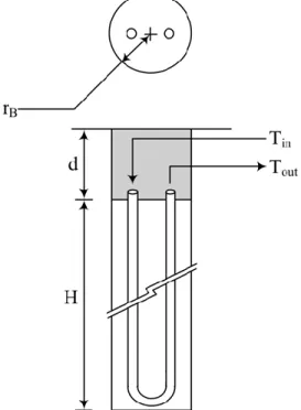
The simulated borehole is a vertical ground heat exchanger, and is shown in Figure 2.1. Its radius and axial extent are respectively rB and H. A U-shape tube is inserted in the
borehole. The pipe has an inner diameter of Dpi and an outer diameter of Dpo. The thermal
conductivity of the pipe material is kp. The space around the pipe in the borehole is filled
Figure 2.1 - Schematic representation of the ground source heat pump system under study.
Chapitre 2 : Article 1 11 with grout, with a conductivity kg. The upper segment of the borehole is assumed not to
exchange heat with the ground over a distance d measured from the surface of the ground (e.g., the fluid collector pipe is located at a depth d). Therefore, the total depth reached by the borehole is H + d, see Figure 2.1. This design represents a typical vertical ground source heat exchanger [21]. This type of geothermal heat exchanger largely dominates the market in the province of Québec, Canada. The values of all parameters and fluid properties used in this work are reported in Table 2.I, and were mostly taken from Ref. [22].
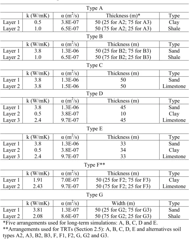
As the present study is concerned with heterogeneous soils, we considered that the ground stratigraphy around the borehole could be characterized by two or three distinct
strata. In other words, the soil thermal conductivity and diffusivity are different in each layer. Fifteen arrangements of heterogeneous soil have been simulated. They are summarized in Table 2.II. The heat transfer modeling of the ground heat exchanger is described below in Section 2.3.
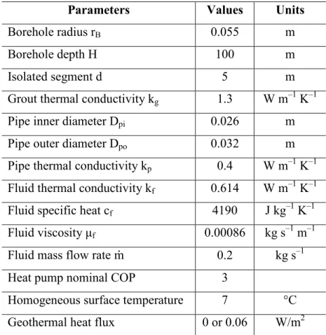
Table 2.I. Values of heat exchanger geometrical and physical parameters. Parameters Values Units
Borehole radius rB 0.055 m
Borehole depth H 100 m
Isolated segment d 5 m
Grout thermal conductivity kg 1.3 W m–1 K–1
Pipe inner diameter Dpi 0.026 m
Pipe outer diameter Dpo 0.032 m
Pipe thermal conductivity kp 0.4 W m–1 K–1
Fluid thermal conductivity kf 0.614 W m–1 K–1
Fluid specific heat cf 4190 J kg–1 K–1
Fluid viscosity μf 0.00086 kg s–1 m–1
Fluid mass flow rate ṁ 0.2 kg s–1
Heat pump nominal COP 3
Homogeneous surface temperature 7 °C
The ground heat exchanger is coupled to a building via a heat pump in order to satisfy the heating and cooling requirement of the building (or a portion of it). The building transient heating/cooling load considered in this work is shown in Figure 2.2. A negative
value represents a heating load and a positive value, the cooling load. This load curve corresponds to a typical residential building located in Quebec City (Canada, longitude =
Table 2.II. Geological environments considered in the simulations.
Type A
k (W/mK) α (m2/s) Thickness (m)* Type
Layer 1 0.5 3.8E-07 50 (25 for A2; 75 for A3) Clay
Layer 2 1.0 6.5E-07 50 (75 for A2; 25 for A3) Shale
Type B
k (W/mK) α (m2/s) Thickness (m) Type
Layer 1 3.8 1.3E-06 50 (25 for B2; 75 for B3) Sand
Layer 2 1.0 6.5E-07 50 (75 for B2; 25 for B3) Shale
Type C
k (W/mK) α (m2/s) Thickness (m) Type
Layer 1 3.8 1.3E-06 50 Sand
Layer 2 3.8 1.5E-06 50 Limestone
Type D
k (W/mK) α (m2/s) Thickness (m) Type
Layer 1 3.8 1.3E-06 45 Sand
Layer 2 0.5 3.8E-07 10 Clay
Layer 3 2.4 9.7E-07 45 Limestone
Type E
k (W/mK) α (m2/s) Thickness (m) Type
Layer 1 3.8 1.3E-06 33 Sand
Layer 2 0.5 3.8E-07 34 Clay
Layer 3 2.4 9.7E-07 33 Limestone
Type F**
k (W/mK) α (m2/s) Thickness (m) Type
Layer 1 1.91 7.0E-07 50 (25 for F2; 75 for F3) Clay
Layer 2 2.43 9.7E-07 50 (75 for F2; 25 for F3) Limestone
Type G
k (W/mK) α (m2/s) Width (m) Type
Layer 1 3.81 1.3E-07 50 (25 for G2; 75 for G3) Sand
Layer 2 2.08 8.6E-07 50 (75 for G2; 25 for G3) Shale
*Five arrangements used for long-term simulations: A, B, C, D and E.
**Arrangements used for TRTs (Section 2.5): A, B, C, D, E and alternatives soil types A2, A3, B2, B3, F, F1, F2, G, G2 and G3.
Chapitre 2 : Article 1 13 71.25, latitude = 46.83), and was determined with a building energy simulation tool [23].
It is important to note that the load of Figure 2.2 is not the load that will be applied to the ground since the coefficient of performance (COP) of the heat pump must be taken into account. For example, in heating mode, the heat taken from the ground is equal to the building load multiplied by (COP – 1)/COP. In general, the exact value of the COP is unknown since it depends on the fluid temperature coming from the ground heat exchangers, which in turn depends on the ground temperature. The heat pump has a nominal COP (Table 2.I) which is assumed here to be the same in heating and cooling mode. In this paper, we assumed that the COP varies with the entering fluid temperature according to [1]:
2
op nom ent ent
COP COP 1.5310 2.2961E 02 T 6.8744E 05 T
(2.1.a) and
2
op nom ent ent
COP COP 1.0000 1.5597E 02 T 1.5931E 05 T
(2.1.b) where Eq. (2.1.a) is for cooling mode, and Eq. (2.1.b), for heating. In these correlations, T is in C.
2.3 Mathematical and numerical model of ground source heat pump system
This section presents the heat transfer model that was used to calculate the heat transfer in the ground and in the heat exchanger. Four heat transfer mechanisms are considered in the mathematical model: convection in the pipe, conduction through the pipe, conduction through grout between the pipe and the ground, and conduction through the ground. Thus, solar radiation, convection on earth surface, and advection due to underground water are not considered in the present model [21].
The conduction equation is used to calculate the temperature and heat flux in the ground. As the borehole has a cylindrical shape and the soil properties vary only in z (i.e. k = k(z)), the 2-D conduction equation in cylindrical coordinates is solved in the ground (i.e., there is no temperature variation with respect to the angular coordinate) [24]:
T 1 T T c kr k t r r r z z (2.2)
The temperature is assumed to be known at the top of the domain (i.e., at z = 0), a fixed heat flux is imposed at the bottom of the domain (i.e., geothermal heat flux at z→∞), and an adiabatic boundary condition is imposed far from the borehole (r→∞) and at r = 0 below the borehole (axisymmetric) [25]. Therefore, the undisturbed temperature profile (at t = 0) is 1D and can easily be calculated from the fixed temperature at z = 0 and the fixed flux at
the bottom. Table 2.I reports the surface temperature and the two values of geothermal heat flux used in this study. At the surface of the borehole (i.e., r = rB, d < z < d+H), a heat flux
distribution is imposed depending on the building need and heat pump COP, as described later.
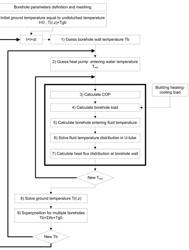
Several numerical heat transfer models have been developed for simulating ground heat exchangers, based on finite volumes [26], finite elements [27] or finite differences [28] [29]. The finite volume method [30] is used here to solve Eq. (2.2) in the ground. The domain is discretized into small control volumes. The mesh is formed of quadrilateral control volumes around the borehole [22] . The domain radial and axial extensions, and the control volume sizing were chosen based on Ref. [25] to ensure mesh independence.
The heat transfer within the borehole itself was modeled based on Ref. [22]. Essentially, the borehole is discretized in many z-layers, each represented by a thermal
Chapitre 2 : Article 1 15 circuit including the thermal short-circuit between the two pipes. The borehole thermal resistance is expressed based on Ref. [31], who proposes an adapted version of the resistance expressions of Ref. [32]. Knowing the temperature of the fluid at the inlet of the U-pipe as well as the temperature distribution at a given time at the surface of the borehole (i.e., at the interface borehole-ground, r = rB), one can calculate the heat flux distribution at
the surface of the borehole by an iterative process, as illustrated in Fig. 2.3. Also, note that at a given time step, the COP is initially unknown since it depends on the fluid temperature which is also unknown, see Eqs. (2.1). Therefore, the required heat transfer rate at the borehole is also unknown and must be found by the iterative procedure (see Figure 2.3; steps 3 to 7). What is imposed is the required amount of heat for the building.
The heat flux and temperature are continuous at the surface of the borehole. Therefore, the overall numerical procedure consisted, at a given time step, in solving the temperature in the ground with an assumed heat flux distribution (Figure 2.3; step 8), then using the resulting surface temperature in the borehole model to update the heat flux
distribution (Figure 2.3; ―new Tb‖ to step 2), and so on, until convergence is achieved, at
which stage it is possible to advance to the next time step. Convergence was declared when the maximal difference of local temperature at the borehole wall was smaller than 0.001°C between two consecutive iterations. Another convergence criterion to respect in the iterative procedure is based on fluid temperature in the U-tube. Fluid temperature is considered converged at a given time step when the difference of heat transfer rate at the borehole surface versus the heat transfer rate calculated with temperature variation through U-tube (energy conservation) is less than 0.001 W.
The code has been validated in different ways. Imposing a constant heat flux on the borehole surface and considering a homogeneous ground, it is possible to compare the code results with analytical solution, such as the line source or cylindrical source solutions. Variations between the numerical and analytical solutions were less than 1.9% for borehole wall temperature after five years of constant heat flux. Also, energy conservation has been verified. According to the first law of thermodynamic, the amount of heat transferred along
the boundaries should be equal to variation of stored energy in the overall volume. To verify it, the sum of heat transfers at the domain boundaries was compared to the variation
Figure 2.3 - Iterative procedure for solving the heat transfer problem and determining the heat pump performance.
Chapitre 2 : Article 1 17 of stored energy in the domain for each year until the tenth year of a simulation. The energy imbalance was always small, below 1%.
2.4 Methodology to assess the impact of stratigraphy
The purpose of the present study is to verify to what extent an average thermal conductivity can appropriately represent a heterogeneous soil in the analysis of a ground heat exchanger. Currently used thermal response tests and sizing procedures are based on analytical solutions to the heat conduction problem for a homogeneous ground, whereas many geological environments are actually highly heterogeneous. A model that can take into account heterogeneity was thus presented in the previous section. The present section explains the methodology used in this paper in order to assess the effects of heterogeneity on thermal response tests and on evaluation of ground coupled heat pumps systems performance.
The average conductivity of the ground is usually determined from a thermal response test (TRT). A typical TRT consists in injecting a fixed heat input in a ground heat exchanger for 2-3 days, and then monitoring the water temperature at the inlet and outlet of the borehole. Afterward, the transient temperature measurements are fitted with an analytical solution (that assumes a uniform conductivity) in order to calculate the average equivalent ground conductivity, i.e. the conductivity value that allows the best match between the data points and the analytical solution. Ground source heat pump systems are then sized based on this value of effective or mean thermal conductivity. However, classical TRTs do not reveal heterogeneity in the ground thermal properties as they simply provide an ―average‖ value.
Usually, in standard TRTs, the line source solution [16] is used to fit the results of the test, which allows to relate the average fluid temperature evolution to the main features of the system. Taking a Taylor series of the infinite line source solution, one finds:
f T (t)a ln(t) b (2.3) where : Q a 4H k B B2 0 Q Q 4 b R ln T H 4H k r (2.4)
Therefore, reporting T tf versus ln(t) in a graph allows to determine the slope, a, and thus, the value of the average ground conductivity, provided that the heat injection rate per unit
of borehole length Q̇ H⁄ is known,
TRT Q
k
4H a
(2.5)
The thermal conductivity of Eq. (2.5) is thus a mean conductivity of the ground around the borehole. In order to evaluate the impact of stratigraphy on this conductivity value, TRTs have been simulated for different geological environments. The geological environments tested are presented in Table 2.II and are based on typical values given in [2]. The rate of heat injection was 4 kW for 72 hours. Eq. (2.5) was then used to extract the mean
conductivity value, just as it would have been for a real in situ TRT. In other words, T (t)f
was plotted against ln(t), and the slope ―a‖ was extracted to calculate kTRT. This value was
then compared with the ground arithmetic mean conductivity. The behavior of the ground heat exchanger in the actual geological environment during the TRT was also compared to that of the same ground heat exchanger that would have been located in a homogeneous medium with the mean conductivity of Eq. (2.5). The results of this analysis are presented in Section 2.5.
Considering that a TRT is typically conducted over a short period compared to the lifetime of a ground heat exchanger(e.g., 2-3 days versus 20 years or more), it is unclear how the actual ground stratigraphy will affect the thermal exchange in the long term when compared to what is calculated by assuming a uniform conductivity. In order to assess the influence of the ground stratigraphy on the design and long-term performance of ground source heat exchangers, the following methodology was employed:
(i) For a given geological environment, the numerical model described above was used to simulate a TRT as explained above.
(ii) The results of each numerical TRT were used to determine the ground average thermal conductivity that would have been determined should a TRT had been conducted in such a geological environment. In order to do so, Eq. (2.5) was used. The values of temperature for the first hours are not considered when evaluating the slope because the analytic solution is not valid for very short times.
Chapitre 2 : Article 1 19 (iii) The long term performance of the ground source heat pump system was simulated with the numerical model described in Section 2.3. The simulation time was 20 years, with the annual load of Figure 2.3 that repeats itself every year. This was done first by using the actual stratigraphy, and second, by assuming a homogeneous conductivity corresponding to that achieved by the numerical TRT for the given stratigraphy. Therefore, in the end, two sets of results per stratigraphy were created and will be compared in the following sections. Note that all cases were tested with the same depth and heat load.
2.5 Influence of stratigraphy on thermal response tests (TRTs)
As mentioned in the previous section, numerical thermal response tests were conducted for the different stratigraphies of Table 2.II. A total constant heat injection rate of 4 kW was simulated for a duration of 72 hours. Environments with and without the presence of a geothermal gradient were considered. For each case simulated, the average temperature of the fluid, i.e. (Tf,i + Tf,o)/2, versus time was determined just as it would have been in a real
in situ test. Then, Eq. (2.5) was used to estimate the effective ground conductivity for each case considered. Values of parameters a and b, values of average thermal conductivity, and values of arithmetic mean thermal diffusivity are given in Table 2.II. The first part of the analysis focuses only on cases without geothermal heat flux. Cases with geothermal heat flux are discussed later.
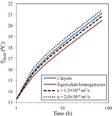
2.5.1 Influence of thermal diffusivity on fluid temperature evolution
Figure 2.4 shows the average fluid temperature as a function of time for a typical TRT (case B, no geothermal gradient). The solid blue curve corresponds to the results of the TRT simulated with the actual stratigraphy (see online version for curves in color). The solid red curve corresponds to the results that would have been achieved for a TRT with a uniform conductivity equivalent to the one found by the TRT realized in the real stratigraphy (i.e. deduced from the solid blue line). It is worth to remember that the conductivity is proportional to the slope of these curves (after the first few hours). Therefore, it makes sense that the slopes be equal for the two solid curves since they both correspond to the same equivalent conductivity. However, an offset shows between the two curves (gap of ~1C for the case presented in Figure 2.4). In other words, although both
systems have the same effective conductivity value, their ‗dynamic behaviors‘ are slightly different.
The difference between the TRT curves with the actual stratigraphy (solid blue) and the homogeneous medium (solid red) can be related to some extent to the variations of thermal diffusivity. When simulating the ground with a homogeneous conductivity, an average diffusivity corresponding to the arithmetic mean was considered. For example, for
the case presented by the solid red curve, the arithmetic mean equaled 9.7×10⁷ m2/s. Figure 2.4 reports the TRT results by varying the homogeneous diffusivity. It can be seen
that a slightly higher diffusivity value (~1.3×10⁶ m2/s) allows to shift the curve in such a
way that it almost matched that of the TRT simulated with the real stratigraphy. It is noted that to obtain a curve perfectly superimposed on the real stratigraphy curve (solid blue), one would have to use an average thermal diffusivity outside the range of those of the two
layers (1.3×10⁻⁶ and 6.5×10⁻⁷ m2/s). However, our goal was not to minimize error between
the measurements and the model by varying the diffusivity, but to explore the impact of neglecting stratigraphy on simulations involving an average value of diffusivity just as one would typically use to perform a borehole simulation. Based on literature, it is essentially
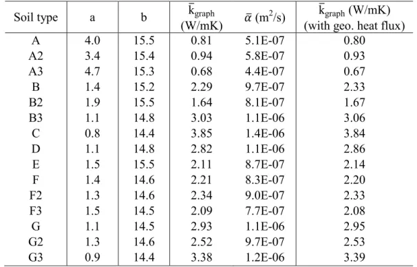
Table 2.III. Fitting parameters and average conductivity from TRT simulations.
Soil type a b k̅graph
(W/mK) ̅ (m
2/s) k̅graph (W/mK)
(with geo. heat flux)
A 4.0 15.5 0.81 5.1E-07 0.80 A2 3.4 15.4 0.94 5.8E-07 0.93 A3 4.7 15.3 0.68 4.4E-07 0.67 B 1.4 15.2 2.29 9.7E-07 2.33 B2 1.9 15.5 1.64 8.1E-07 1.67 B3 1.1 14.8 3.03 1.1E-06 3.06 C 0.8 14.4 3.85 1.4E-06 3.84 D 1.1 14.8 2.82 1.1E-06 2.86 E 1.5 15.5 2.11 8.7E-07 2.14 F 1.4 14.6 2.21 8.3E-07 2.20 F2 1.3 14.6 2.34 9.0E-07 2.33 F3 1.5 14.5 2.09 7.7E-07 2.08 G 1.1 14.5 2.93 1.1E-06 2.95 G2 1.3 14.6 2.52 9.7E-07 2.53 G3 0.9 14.4 3.38 1.2E-06 3.39
Chapitre 2 : Article 1 21 the value of the conductivity that influences the sizing of ground heat exchangers and their long-term behavior [33].
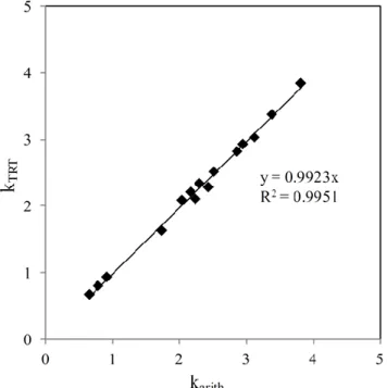
2.5.2 Comparison between average conductivity (TRT) and corresponding arithmetic mean value
The value of the average conductivity based on the numerical TRT for each case tested is plotted against the actual arithmetic averages of the conductivity around the borehole in Figure 2.5. Each point corresponds to a specific stratigraphy and geothermal gradient condition. Points are well distributed around the line kTRT = karith, with a maximal error
around 6% and an average error of 2.7%. The larger difference is noted for the geological environment E which is the more heterogeneous. Also, it is noted that kTRT is typically
larger than karith when the upper layer is more conductive than the bottom layer, and vice
versa. For cases A and F (upper low conductivity layer), the difference between kTRT and
karith increases as the top isolating layer occupies a larger portion of the domain. For
example, for cases A, the larger difference appears when the conductive layer (bottom layer) occupies only 25% of the domain around the borehole (case A3). Also, for these cases, kTRT is always smaller than karith. On the other hand, for cases B and G (upper
Figure 2.4 - Effect of different values of ground average thermal diffusivity on average fluid temperature evolution during a TRT in geological environment B.
conductive layer), the larger difference between kTRT and karith is noted when the interface
between the two strata is located at the mid-height of the borehole, and kTRT > karith.
Furthermore, it is interesting to note that for the cases tested there is a correlation between the percentage of difference between the TRT conductivity and arithmetic mean, and the actual TRT value. The trend is that the error is smaller for environments with
higher thermal conductivity, and vice versa. Future work could focus on the development of a heterogeneity index characterizing an environment and the error associated by representing it by a homogeneous equivalent medium, but that development would involve more research and is out of the scope of the present paper.
2.5.3 Cases with geothermal heat flux
The same analysis was also performed in the presence of a geothermal gradient, and similar results and trends were achieved. Therefore, all details are not reported here. The conductivity achieved by the virtual TRT varied by 2% or less when a geothermal heat flux was imposed, as seen in Figure 2.6, which is within the error range estimated by [15]. When the upper layer was conductive (cases B and G), the effective conductivity was slightly larger in the presence of a geothermal heat flux (see Table 2.III), whereas when the
Figure 2.5 - Average conductivity obtained from numerical TRTs against the actual arithmetic average of the conductivity, for a series of different geological
Chapitre 2 : Article 1 23 upper layer was isolating (cases A and F), the effective conductivity was slightly smaller in the presence of a geothermal heat flux. The maximal difference between the TRT conductivity with and without a geothermal heat flux occurred when the interface separating the two strata was at the middle of the borehole. Overall, with the
actual conditions (no groundwater flow, constant surface temperature), the presence of a typical geothermal heat flux does not introduce major errors on TRT results.
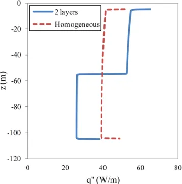
2.5.4 Heat flux distribution at borehole wall
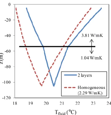
In order to explain further the impact of stratigraphy on TRT results, the heat flux distribution at the borefole surface was also analyzed. For example, Figure 2.7 shows the results achieved for case B at the end of the TRT with no geothermal gradient. The total injection rate is the same for both curves since it is fixed by the TRT procedure. However, the way in which this heat input is distributed over z is very different in both cases. For the real stratigraphy, more heat escapes from the upper layer which is more conductive (67% of the total heat input) while the rest (33%) is dissipated in the bottom layer. The homogeneous model with an equivalent thermal conductivity evaluated that 55% of the heat would escaped from the top part of the domain, and 45% from the bottom portion. Although one could be tempted to use proportionality rules including actual and average
Figure 2.6 - Conductivity obtained from TRT with and without geothermal heat flux.
conductivity values (2.29 W/mK vs. 3.81/1.04 W/mK) to estimate the portion of heat rejected in the upper layer and that in the bottom layer, according to the percentages
obtained (55-45% vs. 67-33%), it appears that due to the fluid temperature distribution in the borehole, one should instead perform a complete simulation to determine how the heat transfer is distributed along the borehole.
2.5.5 Fluid temperature distribution
The fluid temperature distribution in the borehole was also plotted at the end of the TRT. Two curves are reported in Figure 2.8, one for the actual stratigraphy (case B, no geothermal gradient) and one for a homogeneous ground with equivalent thermal conductivity. In the upper layer, the fluid temperature in the U-tube decreases faster in the model with stratigraphy since the conductivity is larger in that layer compared to the homogeneous model. In the second layer, the change of fluid temperature is less important in the stratigraphy model due to a lower conductivity compared to the homogeneous model. Therefore, one can observe that the thermal short-circuit between the two branches of the U-tube is more important for the dashed curve (larger temperature difference between the upper and lower branches over the extent of the tube). The average temperature difference
Figure 2.7 - Heat flux distribution at borewall for case B for simulated TRT of 72 hours.
Chapitre 2 : Article 1 25 between the two branches is 2.0C for the actual stratigraphy, and 2.4C in the homogeneous model. This means that for this stratigraphy (upper layer more conductive, lower layer more isolating, such as cases B and G), a homogeneous model will tend to over-evaluate the short-circuit effect, which would reduce borehole performance to some extent. However, it should be noted that in addition to the effect of the short-circuit, the temperature of the fluid leaving the upward tube is lower with the average conductivity model than for the actual stratigraphy model (likely due to the diffusivity, as discussed above). This lower temperature leads to an overestimation of heat pump performance, resulting actually in an overrated borehole performance. On the other hand, it can be shown that for cases where the upper layer is isolating and the bottom layer is conductive (cases A and F), a homogeneous model will under-evaluate the actual short-circuit effect. Consider, for example, the conductive heat transfer between two cylinders at different temperatures embedded in a medium (grout) can be estimated by [24]:
grout short circuit 2 1 2 po 2 k T q 2w cos 1 D (2.6)
with w being the center-to-center distance between the tubes, and T, the temperature difference between the two branches. With the borehole geometry selected (see Table 2.I) and the average temperature differences noted above, the short-circuit heat transfer rate is estimated at ~5.3 W/m with the actual stratigraphy and at ~6.4 W/m with the homogeneous model, i.e. 20% higher. This might explain why the equivalent conductivity of the TRT was smaller than the arithmetic mean for case B (upper layer more conductive): since the thermal short-circuit is smaller in the actual stratigraphy than in a homogeneous ground, and since the model used to extract the TRT conductivity assumes a homogeneous ground, the TRT procedure tends to underestimate the actual ground conductivity around the borehole.
It is interesting to recall that the short-circuit effect is included in the ground heat exchanger sizing procedure of [2] through a short-circuit factor Fsc ranging from 1 (no
short-circuit) to 1.06 (large short-circuit). This factor multiplies the effective thermal
procedure, the short-circuit factor could eventually depend on the stratigraphy as revealed by the previous discussion.
In summary, the main conclusions related to the influence of stratigraphies on TRTs are:
(i) For the cases tested, there is a difference of up to 6% between the conductivity given by the TRT, and the arithmetic mean of the conductivity around the borehole. Stratigraphy can be a source of error when analyzing thermal response tests with homogeneous models, which adds to uncertainties of measurements and other related errors.
(ii) The thermal short-circuit effect is reduced when the stratigraphy is such that the upper layer is more conductive, when compared to a homogeneous model. Similarly, the thermal short-circuit is increased when the upper layer is more isolating.
2.6 Long-term energy consumption and temperature results for one borehole
The procedure described in Section 2.4 has been applied to stratigraphies A, B, C, D and E of Table 2.II to establish the impact of stratigraphy when evaluating the long-term performance of a ground coupled heat pump system. The simulation results have been analyzed first by looking at the overall energy performance of the ground source heat pump
Figure 2.8 - Fluid temperature distribution for case B for simulated TRT of 72 hours.
Chapitre 2 : Article 1 27 system. The total energy consumed by the heat pump during 20 years is reported in Table 2.IV for stratigraphies A, B, C, D and E based on the two modeling approaches (i.e., simulating the actual stratigraphy versus simulating an average homogeneous conductivity based on TRT results). Results labeled ―Case 1BH-A‖ stand for one borehole simulated into ground type A from Table 2.II, and so on.
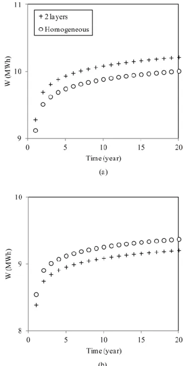
The energy consumption of the heat pump, year per year, for case 1BH-A (case with highest difference between two approaches) is reported in Figure 2.9. The difference between the two modeling approaches is present even after one year, and tends to increase slightly with time. However, the difference is relatively weak.
Overall, the differences in total energy consumption over 20 years between the two modeling approaches are relatively small, between 0.1 and 2.0% depending on the geological environment. This difference can be seen as the error that is generated when simulating the ground source heat pump assuming an average conductivity. The smallest difference was observed for stratigraphy C, corresponding to two layers with the same conductivity but different diffusivities. The highest difference was observed for stratigraphy A (top strata with low conductivity). For the stratigraphies and heat loads studied in this work, predictions of energy consumption based on a TRT average conductivity are found to be relatively precise, irrespectively to the actual heterogeneity.
It is interesting to note that the homogeneous model tends to underestimate the energy consumed by the ground source heat pump system for all cases tested without a geothermal heat flux. In other words, the performance of the ground source heat pump system is slightly overrated by the simulations with a homogeneous ground than with the actual stratigraphy. This overrated heat pump performance is probably linked to the underestimation of fluid temperature as presented in Section 2.5.5. On the other hand, when a geothermal gradient is present, the performance of the ground source heat pump system is underestimated by the homogeneous modeling for case A (upper layer with a low conductivity, see Figure 2.9 b)), and to a lesser extent for case E. Therefore, for most of the geological environments tested, the ―non-consideration‖ of thermal conductivity heterogeneity tends to overpredict the long-term performances of the heat pump system. However, a few environments led to an under-prediction of the performance (in particular, with an isolating first layer and a geothermal heat flux).
Ground heat exchanger sizing is often based on the maximum load that the borehole is able to sustain after a certain period of time. The peak that occurs during the heating season of the twentieth year was considered here as the worst case scenario that the borehole will face as it is that year that the soil temperature is the coldest (since in the
Figure 2.9 - Annual energy consumption for simulations with a single borehole: a) for case in A soil properties with no geothermal heat flux, and b) for case
Chapitre 2 : Article 1 29 present simulation, heating is more important than cooling for the building considered). Therefore, the maximal instantaneous heat transfer rate removed from the ground during the twentieth year (peak load) was also noted and compared for the two modeling approaches; see Table 2.IV. The maximal difference that was reported between the two models is 3.2%. Again, for most cases, the homogeneous model tended to over-predict the peak load carried out by borehole, i.e. to over-predict the performance of the system. The only exception was for case A in the presence of a geothermal heat flux.
Intimately linked to the peak loads is the ground temperature, which will ultimately influence the fluid temperature and the COP of the heat pump. The mean temperature of the ground on the surface of the borehole was also analysed as a function of the modeling approach. For example, the temperature difference between the two models was reported for each stratigraphy at the end of the simulation, i.e. after 20 years of operation. This temperature difference could be seen as a measure of the error that is introduced by using an average thermal conductivity rather than the real thermal conductivity distribution. The local maximal temperature difference between the two models at the same moment was also noted. The average temperature difference varied between 0 and 0.8C depending on the stratigraphy, whereas the maximal local temperature difference could reach up to 4.5C. Large variations of local temperature due to the modeling approach could have an impact in more advanced models that would account of ground water. For example, the homogeneous model could estimate that the temperature is above freezing point, whereas due to stratigraphy, local freezing around the borehole might occur, which could have an impact in terms of heat transfer performance [34]. However, such effect was not accounted for in the present work.
Note that the lower difference between the two models is reached for case C, which has a soil composed of two layers with the same conductivity but different diffusivities. Therefore, the variation of diffusivity has a much smaller impact than variation of conductivity although it can influence long-term performance of GCHP [2].
2.7 Results for a borehole field
Simulations of borefield have also been performed in order to document whether borehole-to-borehole thermal interactions would tend to increase or reduce the effects of stratigraphy