Science Arts & Métiers (SAM)
is an open access repository that collects the work of Arts et Métiers Institute of
Technology researchers and makes it freely available over the web where possible.
This is an author-deposited version published in: https://sam.ensam.eu Handle ID: .http://hdl.handle.net/10985/20268
To cite this version :
Nabeel YOUNAS, Hocine CHALAL, Farid ABED-MERAIM - Finite element simulation of sheet metal forming processes using non-quadratic anisotropic plasticity models and solid-Shell finite elements - Procedia Manufacturing - Vol. 47, p.1416-1423 - 2020
Any correspondence concerning this service should be sent to the repository Administrator : [email protected]
Finite Element Simulation of Sheet Metal Forming Processes using
Non-Quadratic Anisotropic Plasticity Models and Solid−Shell Finite Elements
Nabeel Younas
a,*, Hocine Chalal
a, Farid Abed-Meraim
aaArts et Métiers Institute of Technology, CNRS, Université de Lorraine, LEM3, F-57000, Metz, France
* Corresponding author. Tel.: +33-387375430; E-mail address: [email protected]
Abstract
During the last decades, a family of assumed-strain solid−shell finite elements has been developed with enriched benefits of solid and shell finite elements together with special treatments to avoid locking phenomena. These elements have been shown to be efficient in numerical simulation of thin 3D structures with various constitutive models. The current contribution consists in the combination of the developed linear and quadratic solid−shell elements with complex anisotropic plasticity models for aluminum alloys. Conventional quadratic anisotropic yield functions are associated with less accuracy in the simulation of forming processes with metallic materials involving strong anisotropy. For these materials, the plastic anisotropy can be modeled more accurately using advanced non-quadratic yield functions, such as the anisotropic yield criteria proposed by Barlat for aluminum alloys. In this work, various quadratic and non-quadratic anisotropic yield functions are combined with a linear eight-node hexahedral solid−shell element and a linear six-node prismatic solid−shell element, and their quadratic counterparts. The resulting solid−shell elements are implemented into the ABAQUS software for the simulation of benchmark deep drawing process of a cylindrical cup. The predicted results are assessed and compared to experimental ones taken from the literature. Compared to the use of conventional quadratic anisotropic yield functions, the results given by the combination of the developed solid−shell elements with non-quadratic anisotropic yield functions show good agreement with experiments.
Keywords: Solid−Shell finite elements; Anisotropic plasticity; Sheet metal forming; Deep drawing
1. Introduction
Finite element simulation of sheet metal forming processes is of utmost importance in the field of manufacturing processes being involved in wide spectrum of products. During the last three decades, the development of the numerical techniques has enabled us to predict more accurately the material behavior during the sheet metal forming process. Moreover, quantitative analyses of accuracy of the numerical results show that the choice of constitutive models, which are used in the simulation, has a significant influence on the accuracy of the predicted results. Keeping in the view, advanced material models, which are coupled with efficient finite elements, prove to be optimum solution for the numerical description of complex manufacturing processes, such as sheet metal forming.
During the last few decades, considerable effort has been devoted to the development of solid−shell finite elements for the simulation of thin 3D structures [1-4]. These elements have inherent combined advantages of both shell and solid traditional elements. Recently, a family of solid−shell (SHB) elements has been developed consisting of linear hexahedral (SHB8PS) and prismatic (SHB6) solid−shell elements and their quadratic versions (SHB20 and SHB15, respectively) [3,5-8].
These elements have been found to be performing significantly good for thin structure problems [9-12].
In this paper, the basic formulation of the SHB elements is summarized first; then, different anisotropic plasticity functions, both quadratic (i.e., Hill’48) and advanced non- quadratic (YLD-91, YLD2004-18P) are presented and combined with SHB element to assess their performance for the simulation of deep drawing of a cylindrical cup.
2. Formulation of SHB Solid−Shell elements
In this section, a unified formulation for all SHB solid–shell elements is briefly presented. More details for the formulation of each SHB element can be found in [3,5-8].
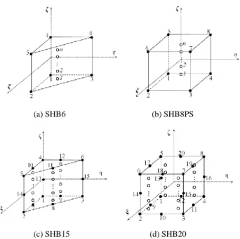
The geometry and location of integration points for SHB8PS, SHB6, SHB20, and SHB15 elements are shown in Fig. 1. The special direction ζ is chosen to represent the thickness direction, along which an arbitrary number of integration points can be arranged. Usually, for non-linear tests involving large strain and plasticity, which is the case of the benchmark tests in this paper, five integration points through the thickness are recommended [5]. see Fig. 1.
(a) SHB6 (b) SHB8PS
(c) SHB15 (d) SHB20
Fig. 1. Geometry and location of integration points for SHB elements: (a) linear prismatic element SHB6 (b) linear hexahedral element SHB8PS (c) quadratic prismatic element SHB15 (d) quadratic hexahedral element SHB20.
The SHB elements are formulated using classical isoparametric linear and quadratic interpolation functions for standard hexahedral and prismatic elements. Accordingly, the three-dimensional position and displacement of any point inside the element, xi and ui (i=1,2,3) respectively, can be
defined using the shape functions NI (I= 1, 2…..., n) as:
1 ( , , ) ( , , ) n i iI I iI I I x x N x N = = =
(1) 1 ( , , ) ( , , ) n i iI I iI I I u d N d N = = =
(2)where xiI and diI denote the Ith nodal coordinate and
displacement, respectively. The lowercase subscript i represents the spatial coordinate directions, while n indicates the number of nodes per element.
The discrete gradient operator B defining the relationship between the strain field us
( )
and the nodal displacement field d is given by:( )
s
u = B d (3)
The SHB element formulation is based on the assumed-strain method, which corresponds to the simplified form of the Hu–Washizu variational principle [13]:
( )
0 e T d T ext =
σ − d f = (4)where represents a variation, ε the assumed-strain rate, σ the Cauchy stress tensor, d the nodal velocities, and ext
f the external nodal forces. The assumed-strain rate ε is defined using a B matrix, which is obtained by projecting the classical discrete gradient operator B involved in Eq. (3):
=
ε B d (5)
Inserting Eq. (5) into the variational principle (Eq. (4)), the element stiffness matrix Keand internal force vector int
f can be derived as: e T ep e=
d+ GEOM K B C B K (6) e int T d =
f B σ (7)where the additional term KGEOM in the expression of the stiffness matrix originates from the non-linear part of the strain field and is commonly called geometric stiffness matrix, while
ep
C is the elastic–plastic tangent modulus associated with the
material behavior law.
In addition to the basic formulation of the SHB elements described above, some special treatments are required for the linear SHB8PS and SHB6 elements in order to improve their performance. In particular, a physical stabilization matrix, computed in a co-rotational coordinate frame [5], is used in the formulation of the SHB8PS element in order to control the zero-energy modes, which are inherent in the reduced-integration technique. Furthermore, an appropriate projection of the strains is required to eliminate some locking phenomena, for the linear SHB6 and SHB8PS elements [5-6].
3. Constitutive equations
The numerical simulation of sheet metal forming processes requires an accurate description of the plastic anisotropy of sheet metals. In order to improve the predicted results, with respect to experimental ones, several anisotropic yield functions have been proposed in the literature. In 1948, Hill introduced the Hill’48 quadratic anisotropic yield function, which is a generalization of the von Mises yield surface [15]. Hill'48 criterion is nowadays one of the most well-known anisotropic yield criteria, and due to its simplicity, it remains as one of the most widely-used yield surfaces for the description of the plastic anisotropy of sheet metals. However, it presents some limitations (being planar anisotropy) for highly anisotropic metals, such as aluminum and titanium alloys, involving the so-called anomalous behavior [16]. Moreover, having a small number of material parameters, Hill’48 yield surface is unable to predict more than 4 ears in the simulation of deep drawing of a cylindrical cup with highly anisotropic materials [17]. The occurrence of more than four ears, which is proved by experimental observations for highly anisotropic sheets, can be predicted only by specific yield surfaces. The latter are based on several anisotropy coefficients, which are identified along different planar directions.
Over the years, Hill has proposed some non-quadratic yield criteria with the aim to properly describe the anisotropy of aluminum alloys [18-20]. Using the concept of linear transformations (i.e., substituting the stress tensor by a modified stress tensor by means of weighting coefficients), Barlat et al. [21] proposed an extension of the isotropic Hershey criterion to orthotropic symmetry, namely Yld91 yield surface, within the framework of three-dimensional formulation. Subsequently, Barlat et al. [22] developed a yield criterion restricted to plane-stress conditions, with eight anisotropy
coefficients and using two linear transformations on the Cauchy stress tensor (namely Yld2000-2d yield criterion). Later, Barlat et al. [23] proposed a criterion within the
framework of three-dimensional formulation, namely
Yld2004-18p yield criterion, using 18 anisotropy coefficients. This high number of anisotropy coefficients was considered also by means of two linear transformations. Due to its high number of anisotropy coefficients, Yld2004-18p yield criterion can correctly predict the behavior of highly anisotropic metals, as shown by Yoon et al. [17]. Several other non-quadratic anisotropic yield criteria were also proposed in the last decades, as can be found in the literature [24-29].
In this work, the formulations of the SHB elements are coupled with various quadratic and non-quadratic yield functions, within the framework of a fully three-dimensional approach, for the simulation of deep drawing of a cylindrical cup with aluminum alloy.
3.1. Constitutive Modeling of yield function
The total strain rate tensor D can be additively decomposed into elastic e D and plastic p D parts as follows: e p = + D D D (8)
In the local material frame, the Cauchy stress rate can be expressed using the following hypo-elastic law:
: ( )
e p
= −
σ C D D (9)
where σ is rate of Cauchy stress tensor and Ce is the fourth-order elasticity tensor. The general form of the plastic yield surface F can be written as:
F =σeq− Y 0 (10)
where σeq is the equivalent stress, which depends on the plastic yield criterion. The isotropic hardening of the material, which characterizes the size of the yield surface, is modeled by the scalar function Y
( )
pl , function of the equivalent plastic strain pl.The plastic strain rate tensor p
D is defined using the classical plastic flow rule, which follows the normality law with respect to the yield surface:
F
p = =
D V
σ (11)
where and V represent the plastic multiplier and the plastic flow direction, respectively.
The plastic multiplier is determined by using the
consistency condition F=0, which leads to the following expression: : : : : e e Y H = + V V C V C D (12)
where the scalar H is the hardening modulus involved in the Y
evolution of the isotropic hardening.
Finally, by substituting the expression of the plastic multiplier into the hypo-elastic law (9), the elasto-plastic tangent modulus is derived as:
ep ( : ) ( : ) : : Y e e e e H + = − C C C V C V V C V (13)
4. Anisotropic yield functions
The present work focuses on the combination of the SHB elements with the following fully three-dimensional anisotropic yield surfaces: the quadratic Hill’48 yield surface for general anisotropic sheet metals, and non-quadratic anisotropic yield functions, namely YLD-91 [21] and YLD2004-18P [23], which are more suitable for the modeling of plastic anisotropy of aluminum alloys. Brief description of each yield function is first presented in this section. Then, they are implemented into ABAQUS software, in conjunction with SHB elements, for the simulation of deep drawing process with a cylindrical cup.
4.1. Barlat’s YLD-91 yield surface
Barlat et al. [21] proposed the YLD-91 plastic yield surface, which is based on a linear transformation of the Cauchy stress tensor. Its expression writes:
2 2 3 3 1
1
F |= S −S |a +|S −S |a +|S −S |a −2Ya 0 (14)
where S1, S2 and S3 are the principal values of tensor S , which is defined as a linear transformation of the Cauchy stress tensor σ:
=
S L σ (15)
where L contains six constant coefficients, which describe the plastic anisotropy of sheet metals. The expression of this linear transformation is given by 2 3 3 2 3 3 1 1 2 1 1 2 4 5 6 0 0 0 0 0 0 0 0 0 1 0 0 0 3 0 0 3 0 0 0 0 3 0 0 0 0 0 0 3 with xx yy zz xy xz yz w w w w w w w w w w w w w w w + + + = = L σ (16)
Hosford [30] and Logan and Hosford [31] have shown that the exponent “a” in Eq. (14) can be equal to 6 and 8 for BCC and FCC metals, respectively. It is worth noting that, when exponent a =2 (or 4) and all coefficients wi are equal to one,
the YLD-91 yield function reduces to the isotropic von Mises yield surface.
4.2. Barlat’s YLD-2004-18P yield surface
Later, Barlat et al. [23] proposed a 3D yield function that involves 18 anisotropy coefficients, which describes accurately
plastic anisotropy of sheet metals. Compared to the YLD-91 yield surface, the non-quadratic YLD-2004-18P yield function is based on two linear transformations of the Cauchy stress tensor. Its expression writes:
(1) (2) (1) (2) (1) (2) 1 1 1 2 1 3 (1) (2) (1) (2) (1) (2) 2 1 2 2 2 3 (1) (2) (1) (2) (1) (2) 3 1 3 2 3 3 F 4 0 a a a a a a a a a a S S S S S S S S S S S S S S S S S S Y = − + − + − + − + − + − + − + − + − − (17)
where S1(1), S(1)2 and S(1)3 are the principal values of the first linearly transformed stress tensor S(1), while (2)
1 S , (2) 2 S and (2) 3
S are the principal values of the second linearly transformed stress tensor S(2). The latter write:
k = (k)
( )
S L S , where k =1,2 (18)
where S = Tσ is the deviatoric part of the Cauchy stress, defined using the transformation matrix T, which is expressed below using voigt’s notation:
2 1 1 0 0 0 1 2 1 0 0 0 1 1 2 0 0 0 1 with 0 0 0 3 0 0 3 0 0 0 0 3 0 0 0 0 0 0 3 xx yy zz xy xz yz − − − − − − = = T σ (19)
The two transformation matrices (1)
L and L used for the (2) two linear transformations contain 18 anisotropy coefficients, and their expressions are:
1 2 3 4 (1) 5 6 7 8 9 0 0 0 0 0 0 0 0 0 0 0 0 0 0 0 0 0 0 0 0 0 0 0 0 0 0 0 c c c c c c c c c − − − − − − = L (20) and 10 11 12 13 (2) 14 15 16 17 18 0 0 0 0 0 0 0 0 0 0 0 0 0 0 0 0 0 0 0 0 0 0 0 0 0 0 0 c c c c c c c c c − − − − − − = L (21)
It should be noted that, by using the same values of coefficients for both transformation matrices 𝐿𝑘, the yield
function YLD 2004-18P reduces to the YLD91 yield surface
accounting for only one linear transformation. Note also that, when the ci anisotropy coefficients in Eqs. (20) and (21) are all
equal to one and a =2 (or 4), the YLD2004-18P yield surface
reduces to the isotropic von Mises yield function [15].
4.3. Hill’48 quadratic yield surface
Hill [14] developed a quadratic yield function for plastic anisotropy, which is an extension of the von Mises yield criterion. The quadratic yield function has the following form:
2 2 2 ( ) + ( ) ( ) + + F xx yy yy zz xx zz 0 xy yz xz F σ - σ G σ - σ σ - σ +2Lσ 2Mσ 2Nσ H Y + = − (22)
where F, G, H, L, M and N are the Hill anisotropy coefficients, which are function of the Lankford coefficients as follows:
(
0)
90 0 1 r F r r = + , 0 1 1 G r = + , 0 0 1 r H r = + , 3 2 L=M = and(
0 90)
45 90 0 (2 1) 2 ( 1) r r r N r r + + = + .It is worth noting that, the Hill’48 yield function reduces to
the isotropic von Mises yield surface when F=G=H =1 2
and L=M =N=3 2. Note also that, being planar orthotropic criterion, the quadratic Hill’48 yield criterion is unable to capture the anisotropy at varying angles to the rolling direction other than 00, 450 and 900. Due to a smaller number of
anisotropy coefficients, Hill’48 yield surface can predict only four ears in the simulation of deep drawing of a cylindrical cup. 5. Simulation of deep drawing of a cylindrical cup
5.1. Description of the finite element model
The above anisotropic yield criteria have been combined with the formulation of SHB elements presented in section 2. The resulting solid−shell elements have been implemented into the finite element code ABAQUS/Standard. The performance of the SHB elements is assessed in this section through the simulation of deep drawing process of a cylindrical cup, involving large strain, anisotropic plasticity, and double-sided contact. The predicted results with SHB elements are compared both with those given by ABAQUS linear solid element with incompatible modes (i.e. C3D8I), using the same constitutive equations presented above, and with experiment measurements taken from the literature.
The geometry and dimensions of the drawing setup are shown in Fig. 2 [17].
Fig. 2. Schematic view for the cylindrical cup drawing process. The material of the sheet is an AA2090-T3 aluminum alloy, with an initial thickness of 1.6 mm. During the simulation, a constant holder force of 22.2kN is applied, and the coulomb friction coefficient associated with the contact between the sheet and the forming tools is taken equal to 0.1.
(a) (b)
Fig. 3. Initial in-plane meshes for one quarter of the circular sheet: (a) prismatic elements and (b) hexahedral elements.
Due to symmetry considerations, only one quarter of the circular sheet is modeled. The quarter of the sheet is meshed with the following nomenclature: N1×N2, where N1 is the
number of elements in the plane of the sheet, while N2 is the
number of elements in the thickness direction. Mesh details for the used finite elements are reported in Table 1.
Table 1. Details of meshes for a quarter of sheet.
C3D8I SHB6 SHB8 SHB15 SHB20
800×3 1350×1 800×1 510×1 255×1
Figure 3 shows the initial in-plane meshes of a quarter of the sheet with prismatic and hexahedral elements. The elasto-plastic parameters associated with AA2090-T3 aluminum alloy are summarized in Table 2, in which the following Swift hardening law has been considered to describe isotropic hardening:
0
pl pl
( ) ( )n
Y
=K +
(23)Table 2. Material properties of Al2090-T3.
E (MPa) K n 0 r0 r45 r90
70,500 0.34 646 0.227 0.025 0.2115 1.5769 0.6923
Anisotropy coefficients for yield functions Hill’48, YLD-91 and YLD2004-18P are reported in Tables 3, 4 and 5, respectively.
Table 3. Hill’48 anisotropy coefficients for Al2090-T3 aluminum alloy.
F G H L M N
0.25217 0.82542 0.17457 1.5 1.5 2.23805
Table 4. YLD-91 anisotropy coefficients for Al2090-T3 aluminum alloy.
w1 w2 w3 w4 w5 w6 a
1.0674 0.8559 1.1296 1.2970 1 1 8
Table 5. YLD2004-18P anisotropy coefficients for Al2090-T3 aluminum alloy. c1 -0.069888 c 11 0.476741 c 2 0.936408 c 12 0.575316 c 3 0.079143 c 13 0.866827 c 4 1.00360 c 14 1.145010 c 5 0.524741 c 15 -0.079294 c 6 1.363180 c 16 1.404620 c 7 0.954322 c 17 1.147100 c 8 1.069060 c 18 1.051660 c 9 1.023770 a 8 c 10 0.981171
Figure 4 shows a qualitative comparison of the geometric shape of the completely drawn cup, as obtained with the linear SHB8PS element, using the Hill’48 and YLD2004-18P yield functions. It can be seen that the linear SHB8PS element predicts four ears with the quadratic Hill’48 yield surface, while six ears are predicted with the YLD2004-18P. The latter results are consistent with the experimental observations for the studied aluminum alloy [23]. Similar results have been obtained with quadratic hexahedral SHB20 element as well as prismatic SHB elements, which are not shown in Fig. 4.
(a) (b)
Fig.4. Final deformed shape of cylindrical cup using SHB8PS element: (a) with Hill’48 yield surface and (b) with YLD2004-18P yield surface.
5.2. Results and discussion
First, for validation purposes, the non-quadratic anisotropic yield function YLD2004-18P has been used to recover the isotropic von Mises criterion using the SHB8PS element. The obtained results, in terms of cup heights, are compared in Fig. 5 to the ones provided with ABAQUS C3D8I element, using the von Mises criterion. As can be seen, no ear has been predicted with both yield surfaces, which is consistent with the isotropic von Mises plasticity model.
Then, the deep drawing of the cylindrical cup is simulated using the SHB elements in conjunction with the three anisotropic yield surfaces (i.e., Hill’48, YLD-91 and YLD2004-18P). The obtained results, in terms of cup heights, are compared in Figs. 6 to 12 with the simulated results using ABAQUS C3D8I element, along with the experimental measurements provided by Yoon et al. [17].
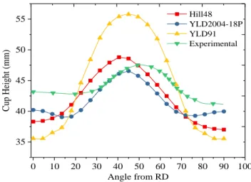
Overall, it can be observed from these figures that the cup height profiles predicted with the quadratic Hill’48 yield surface as well as the non-quadratic YLD2004-18P yield criterion are in good agreement with experimental ones, while the non-quadratic YLD-91 yield surface overestimates the experimental earing profile in the range around the experimental peak value. More specifically, at 0° and 90° from the rolling direction, the predicted cup heights are underestimated with the quadratic Hill’48 yield surface, while the results given by the non-quadratic YLD2004-18P yield criterion are the closest to the experimental heights.
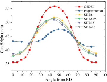
Moreover, although SHB family elements are using only a single element layer through thickness, they are performing more efficiently and accurately than ABAQUS element C3D8I, thus capturing accurate results particularly at 00 and 900 from
the rolling direction, as can be seen in Figs. 11 and 12 for non-quadratic yield surfaces.
In order to compare the computational cost for the deep drawing simulations, the respective CPU times required by the proposed SHB elements and ABAQUS C3D8I element are reported in Table 6 using Hill’48 and YLD2004-18P yield surfaces. This table shows that the CPU times associated with the SHB elements are the lowest, although their computer implementation is not yet optimized.
Table 6. Computation details for the deep drawing of a cylindrical cup.
CPU Time (s) C3D8I SHB6 SHB8PS SHB15 SHB20
Hill48 7773 3412 3199 2514 2239
YLD2004-18P 11221 7413 6201 3856 3499
Fig.5. Predicted cup height profiles obtained using the isotropic von Mises yield surface.
Fig.6. Predicted cup height profiles obtained using ABAQUS C3D8I element: quadratic vs non-quadratic yield surfaces.
Fig.7. Predicted cup height profiles obtained using SHB6 element: quadratic vs non-quadratic yield surfaces.
Fig.8. Predicted cup height profiles obtained using SHB8PS element: quadratic vs non-quadratic yield surfaces.
0 10 20 30 40 50 60 70 80 90 36 38 40 42 44 46 48 Cup H eight (m m) Angle from RD
ABAQUS C3D8I element SHB8PS element 0 10 20 30 40 50 60 70 80 90 100 35 40 45 50 55 Cup H eight (m m) Angle from RD Hill48 YLD2004-18P YLD91 Experimental 0 10 20 30 40 50 60 70 80 90 36 38 40 42 44 46 48 50 52 Hill48 YLD2004-18P YLD91 Experimental Cup H eight (m m) Angle from RD 0 10 20 30 40 50 60 70 80 90 100 36 38 40 42 44 46 48 50 52 Cup He igh t (mm ) Angle from RD Hill48 YLD2004-18P YLD91 Experimental
Fig. 9. Predicted cup height profiles obtained using SHB15 element: quadratic vs non-quadratic yield surfaces.
Fig.10. Predicted cup height profiles obtained using SHB20 element: quadratic vs non-quadratic yield surfaces.
Fig.11. Comparison of cup height profiles obtained with SHB elements and ABAQUS C3D8I element using the YLD2004-18P yield surface.
Fig.12. Comparison of cup height profiles obtained with SHB elements and ABAQUS C3D8I element using the YLD-91 yield surface.
6. Conclusion
In this paper, linear prismatic and hexahedral solid−shell (SHB) elements, along with their quadratic counterparts, have been combined with various advanced anisotropic plasticity models for the simulation of three-dimensional sheet metal forming process of highly anisotropic aluminum alloy. The resulting SHB elements have been implemented into the finite element code ABAQUS/Standard, in the framework of large strain and fully three-dimensional constitutive equations. The performance of the proposed SHB elements has been assessed through the simulation of deep drawing of a cylindrical cup, involving large strain, strong plastic anisotropy, and double-sided contact. The obtained results have been compared with those yielded by ABAQUS solid elements, as well as with experimental results taken from the literature. Compared to the results provided by ABAQUS solid element, the earing profiles predicted by the SHB elements, using non-quadratic yield surfaces, were found to be in good agreement with experiments at lower computational cost. The present work clearly shows that the proposed SHB elements are able to successfully model complex forming process with advanced constitutive equations, using only a single element layer with few through-thickness integration points.
References
[1] Hauptmann R, Schweizerhof K. A systematic development of solid-shell element formulations for linear and nonlinear analyses employing only displacement degrees of freedom. Int J Num Meth Engng 1998;42:49-70. [2] Sze K, Yao L. A hybrid stress ANS solid-shell element and its
generalization for smart structure modeling. Part I: solid-shell element formulation. Int J Num Meth Engng 2000;48:545-564.
[3] Abed-Meraim F, Combescure A. SHB8PS - a new adaptive, assumed-strain continuum mechanics shell element for impact analysis. Comput Struct 2002;80:791-803.
[4] Cocchetti G, Pagani M, Perego U. Selective mass scaling and critical time-step estimate for explicit dynamics analyses with solid-shell elements. Comput Struct 2013;127:39-52.
[5] Abed-Meraim F, Combescure A. An improved assumed strain solid–shell element formulation with physical stabilization for geometric non-linear
0 10 20 30 40 50 60 70 80 90 100 36 38 40 42 44 46 48 50 52 Cup H eight (m m) Angle from RD Hill48 YLD2004-18P YLD91 Experimental 0 20 40 60 80 100 38 40 42 44 46 48 50 52 Cup H eight (m m) Angle from RD Hill48 YLD2004-18P YLD91 Experimental 0 10 20 30 40 50 60 70 80 90 100 38 40 42 44 46 48 Cup H eight (m m) Angle from RD C3D8I Experimental SHB6 SHB8PS SHB15 SHB20 0 10 20 30 40 50 60 70 80 90 100 35 40 45 50 55 Cup H eight (m m) Angle from RD C3D8I Experimental SHB6 SHB8PS SHB15 SHB20
applications and elastic–plastic stability analysis. Int J Num Meth Engng 2009;80:1640-1686.
[6] Trinh V, Abed-Meraim F, Combescure A. A new assumed strain solid– shell formulation “SHB6” for the six-node prismatic finite element. J Mech Sci Tech 2011;25:2345-2364.
[7] Salahouelhadj A, Abed-Meraim F, Chalal H, Balan T. Application of the continuum shell finite element SHB8PS to sheet forming simulation using an extended large strain anisotropic elastic–plastic formulation. Arch App Mech 2012;82:1269-1290.
[8] Abed-Meraim F, Trinh V, Combescure A. New quadratic solid–shell elements and their evaluation on linear benchmark problems. Computing 2013;95:373-394.
[9] Wang P, Chalal H, Abed-Meraim F. Efficient solid‒shell finite elements for quasistatic and dynamic analyses and their application to sheet metal forming simulation. Key Eng Mater 2015;344:651‒653.
[10] Wang P, Chalal H, Abed-Meraim F. Linear and quadratic solid‒shell elements for quasi-static and dynamic simulations of thin 3D structures: Application to a deep drawing process. Stroj Vestn–J Mech Eng 2017;63:25−34.
[11] Wang P, Chalal H, Abed-Meraim F. Quadratic solid–shell elements for nonlinear structural analysis and sheet metal forming simulation. Comput Mech 2017;59:161−186.
[12] Wang P, Chalal H, Abed-Meraim F. Quadratic prismatic and hexahedral solid–shell elements for geometric nonlinear analysis of laminated composite structures. Compos Struct 2017;172:282−296.
[13] Simo JC, Hughes TJR. On the variational foundations of assumed strain methods. J App Mech-T ASME 1986;53:51‒54.
[14] Hill R. A theory of the yielding and plastic Pow of anisotropic metals. In: Proceedings of the Royal Society. London; 1948. p. 281-97.
[15] Mises RV. Mechanik der festen Körper im plastisch-deformablen Zustand. Nachrichten von der Gesellschaft der Wissenschaften zu Göttingen, Mathematisch-Physikalische Klasse. 1913. p. 582-92.
[16] Mellor PB, Parmar A. Plasticity analysis of sheet metal forming. In: Mechanics of Sheet Metal Forming. Boston; 1978. p. 53-77.
[17] Yoon JW, Barlat F, Dick RE, Karabin ME. Prediction of six or eight ears in a drawn cup based on a new anisotropic yield function. IntJ Plasticity. 2006;22(1):174-93.
[18] Hill R. Theoretical plasticity of textured aggregates. In: Mathematical Proceedings of the Cambridge Philosophical Society. Cambridge; 1979. p. 179-91.
[19] Hill R. Constitutive modelling of orthotropic plasticity in sheet metals. J Mech Phys Solids 1990;38:405-17.
[20] Hill R. A user-friendly theory of orthotropic plasticity in sheet metals. Int J Mech Sci 1993;15:19-25.
[21] Barlat F, Lege DJ, Brem JC. A six-component yield function for anisotropic materials. Int J Plasticity 1991;7:693-712.
[22] Barlat F, Brem JC, Yoon JW, Chung K, Dick RE, Lege DJ, Pourboghrat F, Choi SH, Chu E. Plane stress yield function for aluminum alloy sheets. Part 1: theory. Int J Plasticity 2003;19:1297-1319.
[23] Barlat F, Aretz H, Yoon JW, Karabin ME, Brem JC, Dick RE Linear transformation-based anisotropic yield functions. Int J Plasticity 2005; 21:1009-1039.
[24] Bassani JL. Yield characterisation of metals with transversally isotropic plastic properties. Int J Mech Sci 1977;19:651-4.
[25] Gotoh M. A theory of plastic anisotropy used on a yield function of fourth order. Int J Mech Sci 1977;19:505-20.
[26] Barlat F, Richmond O. Prediction of tricomponent plane stress yield surfaces and associated Pow and failure behavior of strongly textured FCC polycrystalline sheets. Mater Sci Eng 1987;91:15-29.
[27] Barlat F, Lian J. Plastic behavior and stretchability of sheet metals. (Part I). A yield function for orthotropic sheet under plane stress conditions. Int J Plasticity 1989;5:51-6.
[28] BUDIANSKY B. Anisotropic plasticity of plane-isotropic sheets. In: Studies in Applied Mechanics. 1984. p. 6:15-29.
[29] Barlat F, Becker RC, Hayashida Y, Maeda Y, Yanagawa M, Chung K, Brem JC, Lege DJ, Matsui K, Murtha SJ, Hattori S. Yielding description for solution strengthened aluminium alloys. Int J Plasticity 1997;13:185-401.
[30] Hosford WF. A generalized isotropic yield criterion. J Appl Mech-T ASME 1972;39:607-609.
[31] Logan RW, Hosford WF. Upper-bound anisotropic yield locus calculations assuming pencil glide. Int J Mech Sci 1980;22:419-430. [32] Grilo TJ, Valente RAF, Alves de Sousa RJ. Assessment on the
performance of distinct stress integration algorithms for complex non-quadratic anisotropic yield criteria.Int J Mater Form 2014;7:233-247.