Ballistic behavior of steel sheet subjected to impact and perforation

Science Arts & Métiers (SAM)

is an open access repository that collects the work of Arts et Métiers Institute of Technology researchers and makes it freely available over the web where possible.

This is an author-deposited version published in: https://sam.ensam.eu Handle ID: .http://hdl.handle.net/10985/9619

To cite this version :

Tomasz JANKOWIAK, Alexis RUSINEK, K. M. KPENYIGBA, Raphaël PESCI - Ballistic behavior of steel sheet subjected to impact and perforation - Steel and Composite Structures - Vol. 16, n°6, p.595-609 - 2014

Any correspondence concerning this service should be sent to the repository Administrator : archiveouverte@ensam.eu

Ballistic behavior of steel sheet

subjected to impact and perforation

Tomasz Jankowiak

, Alexis Rusinek

, K.M. Kpenyigba

, Raphaël Pesci

Institute of Structural Engineering, PUT, Poznan, Poland

2

LaBPS, National Engineering School of Metz, Metz, France

3

LEM3 UMR CNRS 7239, ENSAM-Arts et Métiers ParisTech CER of Metz, Metz, France

Abstract.  The paper is reporting some comparisons between experimental and numerical results in terms

of failure mode, failure time and ballistic properties of mild steel sheet. Several projectile shapes have been considered to take into account the stress triaxiality effect on the failure mode during impact, penetration and perforation. The initial and residual velocities as well as the failure time have been measured during the tests to estimate more physical quantities. It has to be noticed that the failure time was defined using a High Speed Camera (HSC). Thanks to it, the impact forces (average and maximum level), were analyzed using numerical simulations together with an analytical description coupled to experimental observations. The key point of the model is the consideration of a shape function to define the pulse loading during perforation.

Keywords:   impact; perforation; dynamic failure; experiment; simulation; impact force

1. Introduction

The paper describes the behavior of mild steel sheets under extreme loading conditions. Previously, the topic was developed by many authors as for example Zukas and Sheffler (2001). The authors analyzed the perforation of the monolithic and multi-layered slabs using two descriptions of deformations: Lagrangian and Eulerian. It was illustrated that Lagrangian formulation predicts more accurate results than Eulerian when comparing experimental data with analytical solutions. Scheffler and Zukas (2000) analyzed the influence of two numerical methods: finite difference (FD) and finite element (FE) on numerical results for fast dynamic problems. The authors illustrated the origin of the discrepancy in numerical results. The distribution of nodes (FD), shape and type of elements (FE) were taken into account. The authors also previously described the effect of the contact interaction formulation and the constitutive material description (strain rate sensitivity type) on the dynamic behavior of the metal sheets (Scheffler and Zukas 2000). Dean et al. (2009) analyzed the ballistic properties of thin steel sheets using Abaqus/ xplicit

finite element code for projectile impact velocities between 200 and 600 /s. The energetic balance during the penetration and perforation of the structure by hemispherical projectiles was illustrated using the shell finite elements description for steel sheets. Lee and Wierzbicki (2005) presented the propagation of radial cracks in thin metal sheets during impact by impulsive loads. The authors analyzed the influence of the triaxiality on the failure pattern using the shell elements for impacted structure. Atkins et al. (1998) analyzed the formation of radial cracks around the perforation zone in aluminum sheets. The influence of the small hole in the impacted area was taken into account for both conical and hemispherical projectiles. The authors observed that the appearance of the cracks is preceded by the creation of necks; the number of cracks is smaller than the number of necks. Other authors analyzed the perforation of thick plates. Borvik et al. (2002) presented the influence of the projectile end shape on the failure pattern during perforation of 12mm steel sheets (Weldox 460 E). They illustrated the influence of the projectile shape on the absorbed energy. A lower energy is absorbed during impact of a blunt projectile, Fig. 1. Dey et al. (2004) analyzed the perforation of12mm steel plates for different types of Weldox steel.Different shapes of projectiles were studied, and their influence on the ballistic properties was illustrated. The identification of the material parameters based on different tests was presented by Dey et al. (2004) considering both static and dynamic measurements (Jankowiak et al. 2011). Some other authors analyzed the multilayered structures perforated by hemispherical projectiles. Alavi Nia and Hoseini (2011) described that monolitic structures were much more resistant to perforation (lower residual velocity and higher ballistic limit) than multilayered. Jankowiak et al. (2013) presented a numerical study of the perforation process of mild steel sheets for conical projectiles. The authors studied different configurations of steel sheets, including multilayered), and the two constitutive models: Rusinek-Klepaczko (Rusinek et al. 2007) and Johnson-Cook (Johnson and Cook 1983). The effects of the material behavior, strain rate sensitivity, yield stress and strain hardening were illustrated. Recht and Ipson (1963) presented an analytical equation for approximation of the ballistic curve. It was validated for perpendicular and oblique impacts using different projectile shapes. Using several experimental works allowing to define the shape of the force pulse (Minak and Ghelli 2008, Bektaş and Ağır 2013), it is possible to estimate different forces imposed to the structure studied. The force estimation is a quantity which can be linked to the strain rate sensitivity of the materials as discussed in (Jankowiak et al. 2011).

This paper describes extensions of the previous works and presents an analysis based on the failure time and impact force for different kinds of projectiles. It contains three main parts: experimental, numerical and analytical description.

2. Experimental part

The experimental technique is presented in details below. All tests are performed to describe the ballistic dynamic behavior of the steel sheets. Finally the three main experimental variables like the initial impact velocity, the residual impact velocity and the failure time are used to predict the average impact force assuming a constant projectile deceleration and the maximum force level induced to the plate.

2.1 Description of experiments

The tested structures are mild steel sheets 130×130mm2 _{in size with a thickness equal to 1 mm.}

Fig. 1 Geometry of the impacted and perforated sheet steel and projectile shape used

Fig. 2 Experimental setup for ballistic applications

dimensions are reported in the figure. The perforation process can be divided into three main stages which are defined by the position of the projectile.

• impact on the structure,

• penetration of the structure (initially only projectile nose), • perforation of the structure.

The process is carefully recorded using a High Speed Camera (HSC) Phantom v711 during experiments.

The device, and more precisely the gas gun, used to perform the tests (Kpenyigba et al. 2013) is instrumented with two laser sensors allowing to measure the initial velocity V0 and two laser

barriers to measure the residual velocities VR, see Fig. 2. The laser barriers allow to detect a

minimum projectile size of 5 mm. The experiments are performed using three projectile shapes: conical, hemispherical and blunt, see Fig. 1. The mass of the projectile is assumed constant and

equal to 30 g to have the same kinetic energy for an imposed impact velocity. The contact between the steel sheet and the projectile is considered as dry. The two velocities measured during the experiments are used to define the ballistic curve VR - V0. The minimum initial velocity for which

the projectile perforates the sheet steel is called ballistic limit VB. The residual velocities can also

be measured using HSC so that a comparison is possible with lasers. In addition, the camera allows to define the failure time tf for all projectile shapes.

2.2 Results of experiments

Two series of experiments are performed for all three projectile shapes. First, the ballistic curves are obtained using laser sensors. The second series of experiments are performed using HSC to record the perforation process allowing to calculate the failure time for velocities higher than the ballistic limit. Finally, it is possible to calculate the deceleration time of the projectile, also called the failure time, during perforation using HSC.

From all the recorded experiments, only some frames are reported in the paper, Figs. 3, 4 and 5, to explain the basic effects. Fig. 3 refers to a blunt projectile and presents three frames corresponding to the perforation process. The velocity measured by the initial velocity sensor is 88.65 m/s and the residual velocity measured using the HSC is equal to 53.6 m/s. On the left, the

Vo = 88.65 m/s VR = 53.6 m/s (HSC)

(a) 30 μs - impact (b) 151 μs - penetration (c) 182 μs - perforation Fig. 3 Perforation process - mild steel sheet perforated by blunt projectile

Vo = 73.53 m/s VR =16.5 m/s (HSC)

(a) 30 μs - impact (b) 242 μs - penetration (c) 515 μs - perforation Fig. 4 Perforation process - mild steel sheet perforated by conical projectile

Vo = 84.75 m/s VR = 3.2 m/s (HSC)

(a) 30 μs - impact (b) 363 μs - penetration (c) 727 μs - perforation Fig. 5 Perforation process - mild steel sheet perforated by hemispherical projectile

(a) (b)

(c)

Fig. 6 Ballistic curves - experimental data: (a) Blunt projectile; (b) Conical projectile; (c) Hemispherical projectile

frame just after impact (30 μs) is visible; on the right, the frame with complete perforation (the projectile nose reaches the opposite side of the sheet) is presented (182 μs). In addition, an intermediate frame (151 μs) is reported to present the failure evolution during penetration. During perforation, the projectile decelerates from initial to residual velocity in a very short time (182 μs). It is possible to predict the impact force level which is transferred from the projectile to the plate as it will be discussed later.

Next figure, Fig. 4, reports the three corresponding frames for a conical projectile considering an initial impact velocity equal to 73.53m/s.The residual velocity given by HSC is 16.5m/s. Fig. 5 presents the corresponding experimental results for a hemispherical projectile. In this case, the residual velocity is 3.2 m/s for an initial velocity equal to 84.75 m/s. This low residual velocity means that the initial impact velocity is close to the ballistic limit.

Finally, in Fig. 6, the ballistic curves for all the considered projectile shapes are summarized. The ballistic limits are also reported. The data from velocity sensors discussed previously, Fig. 2, together with HSC (one point for every projectile shape) are compared. Using experimental results, the relation proposed by Recht and Ipson (1963) is used to fit the experiments. A good agreement is observed in all cases.

Different mechanisms of failure are observed during experiments (Kpenyigba et al. 2013) using conical, hemispherical and blunt projectiles, Figs. 3, 4 and 5. The conical projectile presented has an angle of 72°, Fig. 1, but other angles have also been considered. The experiments have shown that increasing the projectile angle induces a decrease of the number of petals until a critical angle of 120° beyond which a plug ejection is observed. The detailed presentation of this effect is described in (Kpenyigba et al. 2013).

3. Numerical part

Some numerical simulations with Abaqus/Explicit finite element code (Simulia 2011) have been done to predict among others the failure mode, the ballistic curve and the ballistic limit, and to compare with the experimental results. In addition, some specific analyses to define the impact force history based on analytical approach have been carried out.

3.1 Numerical model description

The numerical simulations are used to describe in particular the aspects of the experiments which cannot be measured directly in the laboratory, for example the impact force (no sensors fixed on the set-up), stress, strain, displacement and velocities distribution during the process. The numerical model used in simulations is presented together with boundary and initial conditions. In addition, the constitutive material model is given with the material parameters.

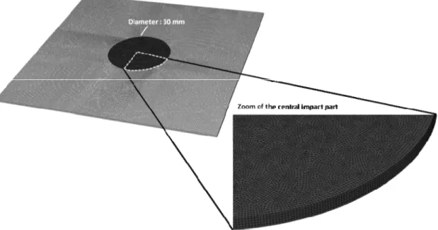
The explicit finite method is used to integrate in time domain the equations of motion. Finally, the process of impact, penetration and perforation is simulated; the finite element mesh is shown in Fig. 7. The central part of the model is built with about 110,000 finite elements (five elements along thickness: type C3D8R, size 0.2 mm) and the exterior part has about 73 000 elements (two elements along thickness: type C3D8I, size 0.5 mm). It means that the length of the finite elements is 0.2 mm in the central zone and 0.5mm in the exterior zone. C3D8I are used to model in a better way the bending behavior of the plate. The tie constraint guarantees a continuous displacement and stress fields on the border. The fine mesh in the interior zone of the model is 30mm in diameter. It allows initiating the crack propagation in a precise way. The mesh density in the impacted zone

Fig. 7 Finite element mesh used to simulate the process

has also been analyzed to avoid the effect of the mesh sensitivity on the numerical results (Jankowiak et al. 2013). Borvik et al. (2002) used the same mesh density – it means the mesh size is optimal. The projectile is defined using C3D8R (hexahedral) and C3D10M (tetrahedral) elements type. The second type is mainly used to discretize the front of the projectile (in case of conical and hemispherical projectile). All elements of the projectile are constrained as a rigid non deformable body. This assumption is in agreement with experiments since the projectile is machined using a maraging steel with a yield stress close to 2 GPa. During numerical simulations the sheet steel is fixed along the perimeter to induce a complete embedding of the plate as during experiments. Moreover, the projectile is launched with an initial impact velocity as during the tests. The velocity is decreased during the process of impact and perforation depending on the mechanical properties of the sheet steel described below. The contact used between the projectile and the plate is based on a penalty formulation with contact pair. Moreover, a contact restriction is defined between the outer surface of the projectile and the interior and exterior nodes of the plate to keep the interaction during the process of perforation.

The mild steel material behavior is modeled using a thermoviscoplastic formulation which take into account strain hardening, strain rate sensitivity and thermal softening. In numerical simulations, the isotropic hardening-softening law proposed by Johnson-Cook (Johnson and Cook 1983) was used in the following form, Eq. (1). Other sophisticated constitutive models exist and can also be used to model the perforation process (Abed and Voyiadjis 2005, Zerilli and Armstrong 1987, Rusinek et al. 2007).





Table 1 All constants used for the Johnson-Cook model, Eqs. (1) and (2)

A (MPa) B (MPa) n (-) C (-) ε˙0 (s-1) Ttrans (K) Tmelt (K) m (-)

153.82 463.82 0.37 0.02 0.0001 300 1600 0.7

β (-) Cp (Jkg-1_K-1_{) ρ (kgm}-3₎

0.9 470 7800

Table 2 Failure strain and triaxiality for each projectile shape

Projectile shape Blunt Conical Hemispherical

Failure strain εf 0.6 1.2 0.65

Average triaxiality η¯ 0 1/3 2/3

where σ is the equivalent von-Mises stress, εp is the equivalent plastic strain, ε˙p is the equivalent

plastic strain rate and T is the actual temperature. The model has five material parameters A, B, n,

C and m that describe the yield stress (A), the strain hardening (B and n), the strain rate sensitivity

(C) and the thermal softening (m). In addition, the following physical properties should be identified: Tmelt (melting temperature), Ttrans (transition temperature) and the reference strain rate ε˙0.

The increment of temperature assuming adiabatic conditions is calculated based on the following equation, Eq. (2) ,



the specific heat.

The constants used to describe the thermoviscoplastic behavior of the mild steel are summarized in Tables 1 and 2. This allows to take into account strain, strain rate and temperature sensitivity.

It must be noticed that the residual velocity depends on the failure strain level εf. It is an

important variable; a sensitivity analysis is done for all three shapes of projectile, Fig. 9. The optimal values of the failure strains are presented in Table 2 for each projectile shape. When the local equivalent strain reaches these values, the elements are deleted but the nodes are still active in the model to assume a constant mass. During numerical simulations of perforation, the average triaxiality η¯ has been estimated, see Table 2. The triaxiality η¯ is defined as the ratio of ‒ p and q, where p is the hydrostatic stress (first invariant of the stress tensor) and q is the Huber-Mises equivalent stress (second invariant of stress deviator). During numerical simulation an average value of η¯ has been defined locally. Thus, it is observed that for a blunt projectile failure mode is dueto pure shear(η¯=0);for conical,it is related to uniaxial tension (η¯=1/3) and for hemispherical to biaxial tension (η¯=2/3). All these observations are in agreement with the results presented by Lee and Wierzbicki (2005) and by Bao and Wierzbicki (2005).

3.2 Numerical results

It is possible to reproduce numerically all the failure modes observed during experiments, Figs. 3, 4 and 5. The numerical and experimental results are in good agreement, Fig. 8. The number of

Fig. 8 Failure pattern for conical, hemispherical and blunt projectile shapes, V0 = 120 m/s

(a)

(b) (c)

petals with the projectile nose angle between 30° and 120° is well reproduced as reported by Kpenyigba et al. (2013). The ballistic curves considering all projectile shapes are also well defined, Fig. 9.

As described in Tab. 2 the best correlations between experimental and numerical results are for a failure strain level εf equal to 0.6 for a blunt projectile, 1.2 for a conical projectile and 0.65 for a

hemispherical shape.

Using numerical simulations, the ballistic curves have been defined to validate this approach for a large range of impact velocity. The ballistic properties of the plate considered is mainly defined using VR ‒ V0, Fig. 9.

It is observed that only using a hemispherical projectile the ballistic limit is increased to 83 m/s in comparison with two other cases having an average value of 71 m/s. The definition of the residual velocity is a key point mainly to estimate in a correct range the average force imposed to the plate and also the maximum force induced. This point is discussed in the point 3.4.

3.3 Failure time

The important aspect analyzed very often during the perforation process is the failure time, it means the time for complete perforation of the plate as it is defined on the right side of Figs. 3, 4 and 5. The time resolution of high speed camera is about 30 μs but the resolution of the numerical model depends on the initial velocity. During our perforation tests, it corresponds to 20 frames but of course the process is shorter for higher initial velocities and longer for lower impact velocities. Finally, the time resolution of numerical simulations is between 10 μs and 50 μs.

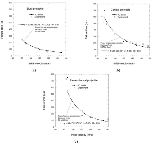
The curves describing these relationships for all three considered projectile shapes are presented in Fig. 10. The agreement is acceptable taking into account possible errors from time resolution of the HSC and the numerical model. The important idea is that the same methodology is used for both types of analyses and provides consistent results.

Taking into account the initial impact velocity (higher or equal to the ballistic limit), the residual impact velocity associated and the failure time described for all three projectile shapes, it is possible to predict the average total force (TF). Based on it, the force history may be estimated thanks to the previous quantities even if no force sensors were used during the tests.

Using the previous results, Fig. 10, it is observed that the shorter failure time is obtained using a blunt projectile due to the process of high speed cutting.

3.4 Impact force

The force-time histories produced by the penetration into the target are also analyzed in this paper. During previous experiments, it was not possible to measure the force because of a lack of appropriate equipment. However the numerical study allows to predict the impact force which is generally a nonlinear impulse during perforation, see Fig. 11. As discussed above, it is possible to describe some points on the ballistic curve for which coordinates are initial velocity V0 and

residual velocity VR, see Fig. 9. The perforation time can also be described using HSC. It is related

to the deceleration of the rigid projectile, Fig. 10 and is defined as the minimum time after loading to reach a force F and a rate force F˙ equal to zero. However using a simple approach based on both initial impact velocity and residual velocity, it is possible to estimate the average force imposed to the plate specimen, Eq. (3). The failure time is defined using as reference the moment when the projectile starts to be in contact with the plate, tF = t ‒ tcontact.

(a) (b)

(c)

Fig. 10 Comparison of failure time in experiments and numerical simulations for different projectile shapes Table 3 Data for impact force analysis

Type Initial velocity _(m/s) Residual velocity _(m/s) Max FH _(N) MTP_(μs) OTP _{(μs) (N)} AF _(N)TF

Simulation 88.000 23.040 9310 490 - 3820 - Experiment 87.720 23.830 - - 545 - 3516 Simulation 121.00 93.770 9620 190 - 4070 - Experiment 121.95 89.16 - - 242 - 4065 *Notation: FH – Force History

MTP – Measured Time of Perforation OTP – Observed Time of Perforation AF – Average Force (from FH) TF – Theoretical Force

(a) Impact velocity 88 m/s (b) Impact velocity 121 m/s Fig. 11 Predictions of the impact force for hemispherical projectile

The average theoretical force TF, assuming the constant deceleration, imposed to the structure during impact can be calculated from experiments, based on the following formulation

. 0 p F R _m t V V TF   (3)

In the previous case (hemispherical projectile and low impact velocity – 88 m/s), Table 3, all necessary data (V0, VR, tF) are reported and the mass of the projectile is 30 g. The theoretical force

(TF) is 3516 N in experiment and 3820 N in simulation (AF). For a higher velocity close to 121m/s, the theoretical force (TF) is 4065 N in experiment and 4070 N in simulation. It is visible that the assumption about a constant deceleration during experiment describes correctly the quantity defined.

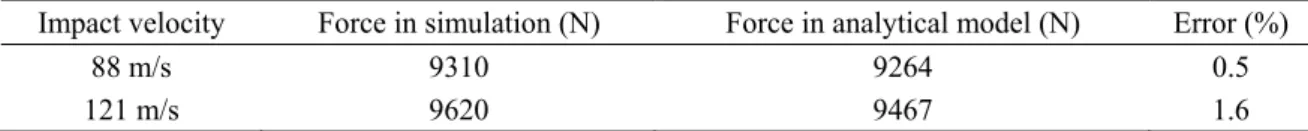
The maximum forces obtained from simulations are 9310 N and 9620 N, respectively, and are higher than TF and AF. Assuming that the force impulse has a nonlinear behavior (Hockauf et al. 2007, Rusinek et al. 2008, 2009, Bektaş and Ağır 2013, Minak and Ghelli 2008), it is possible to use a shape function as bilinear, polynomial, exponential, among others. However, it is observed as described in the previous papers that a parabolic shape allows to mimic experimental result observations. For this reason, the shape function used to fit the impact force Fi(t) is described

using the following equation

. )

(t at bt2

F_i   (4)

The parameters a and b are calculated using a minimization method linked to the theoretical force (TF). The following minimization problem

0 0 1 , ( ) , and 1 arg min V V t V V t F m _F R R m n i b a _        _ 



0 0 0          if if (6) In fact, the force imposed cannot be negative and it is satisfied thanks to Eq. (6). Moreover the force expression must satisfy the following boundary limits

0 ) ( 0 ) 0 (   F t F F (7) Even if the pulse is not completely defined mainly after reaching the maximum force, it is observed that the maximum predicted from numerical simulations is in agreement with that from the simplified approach, Eqs. (4)-(5), see Fig. 12. Of course, the prediction is depending on the shape pulse function definition. In the case here presented, the convergence was defined when the difference equation, Eq. (5) was less than 1%. The time resolution used to define the force Fi(t)

and to generate the data base was fixed to 2 μs. The data base density is an important parameter for the process of optimization.

The constants a and b are defined in the following table, Table 4. It is observed that the values are depending on the initial impact velocity, to define in fact the loading time decrease and the force increase corresponding for example to the strain rate sensitivity of the material.

Using the previous results, a comparison has been performed based on the maximum force level. It is observed that even if the average force difference was kept constant and equal to 0.1%

Table 4 Definition of the parameters a and b for both impact velocities

Impact velocity a (N/s) b (N/s2₎

88 m/s 1.22e8 -4e11

121 m/s 3.16e8 -2.64e12

(a) Impact velocity 88 m/s (b) Impact velocity 121 m/s Fig. 12 Comparison of simulated and analytical force using Eq. (5) for hemispherical projectile

Table 5 Comparison in term of maximum forces and error estimation

Impact velocity Force in simulation (N) Force in analytical model (N) Error (%)

88 m/s 9310 9264 0.5

121 m/s 9620 9467 1.6

during the process of optimization, the maximum force error is changed, Table 5. It is observed that the two areas are compensated after the maximum for level due to the force nature. Therefore, the error is mainly due to this effect. It has to be noticed that the force will drop quickly increasing the initial impact velocity and the linear decrease will vanish (Rusinek et al. 2009). In this case, the model will predict in a better way experimental results.

If the failure time tF during experiments is defined precisely using a HSC, it is possible to

estimate a maximum force level and an average force imposed to the impacted structure, Eq. (3) and Eqs. (4)-(7). In addition, the time corresponding to the maximum force level can be estimated as reported in Fig. 12.

4. Conclusions

In this paper, a complete analysis of the perforation process is reported. Coupling an experimental approach to numerical simulations, fundamental quantities can be measured and analyzed. It allows a better understanding of the perforation mechanisms. Moreover, a good agreement is observed between experiments and numerical results.

Through experiments, it is observed that the projectile shape is changing the failure mode and the failure strain level. It is due to the stress triaxiality state as reported in (Kpenyigba et al. 2013). The failure time is studied and in all cases, a parabolic decrease with the impact velocity is observed. It is also observed during the tests that the nose angle of a conical shape is changing the number of petals corresponding to radial cracks.

In addition, based on failure time as well as initial and residual velocities, the impact force is predicted (numerically and experimentally). The real time history of the impact force is also defined in simulations and obtained analytically using an optimization method together with common experimental data like initial impact velocity, residual projectile velocity and failure time.

Acknowledgments

Authors thank the Polish Ministry of Science and Higher Education for financial support under the grant Demonstrator+ WND-DEM-1-203/00.

References

Abed, F.H. and Voyiadjis, G.Z. (2005), “Plastic deformation modeling of AL-6XN stainless steel at low and high strain rates and temperatures using a combination of bcc and fcc mechanisms of metals”, Int. J.

Plasticity, 21(8), 1618-1639.

hemispherical-nosed projectiles”, Mater. Des., 32(2), 1057-1065.

Atkins, A.G., Afzal Khan, M. and Liu, J.H. (1998), “Necking and radial cracking around perforations in thin sheets at normal incidence”, Int. J. Impact Eng., 21(7), 521-539.

Bao, Y. and Wierzbicki, T. (2005), “On the cut-off negative triaxiality for fracture”, Eng. Fract. Mech., 72(7), 1049-1069.

Bektaş, N.B. and Ağır, İ. (2013), “Impact response of composite plates manufactured with stitch-bonded non-crimp glass fiber fabrics”, Sci. Eng. Compos. Mater., 21(1), 111-120.

DOI: 10.1515/secm-2012-0066

Borvik, T., Langseth, M., Hoperstad, O.S. and Malo, K.A. (2002), “Perforation of 12 mm thick steel plates by 20 mm diameter projectiles with flat, hemispherical and conical noses part I: experimental study”, Int.

J. Impact Eng., 27(1), 19-35.

Dean, J., Dunleavy, C.S., Brown, P.M. and Clyne, T.W. (2009), “Energy absorption during projectile perforation of thin steel plates and the kinetic energy of ejected fragments”, Int. J. Impact Eng., 36(10-11), 1250-1258.

Dey, S., Borvik, T., Hopperstad, O.S., Leinum, J.R. and Langseth, M. (2004), “The effect of target on the penetration of steel plates using three different projectile nose shapes”, Int. J. Impact Eng., 30(8-9), 1005-1038.

Hockauf, M., Meyer, L.W., Pursche, F. and Diestel, O. (2007), “Dynamic perforation and force measurement for lightweight materials by reverse ballistic impact”, Composites: Part A, 38(3), 849-857. Jankowiak, T., Rusinek, A. and Lodygowski, T. (2011), “Validation of the Klepaczko–Malinowski model

for friction correction and recommendations on Split Hopkinson Pressure Bar”, Finite Elements in

Analysis and Design, 47(10), 1191-1208.

Jankowiak, T., Rusinek, A. and Wood, P. (2013), “A numerical analysis of the dynamic behaviour of sheet steel perforated by a conical projectile under ballistic conditions”, Finite Elem. Anal Des., 65, 39-49. Johnson, G.R. and Cook, W.H. (1983), “A constitutive model and data for metals subjected to large strains,

high strain rates and high temperatures”, Proceedings of 7th _{International Symposium on Ballistics, Hague,} the Netherlands, April.

Kpenyigba, K.M., Jankowiak, T., Rusinek, A. and Pesci, R. (2013), “Influence of projectile shape on dynamic behavior of steel sheet subjected to impact and perforation”, Thin-Wall. Struct., 65, 93-104. Lee, Y.W. and Wierzbicki, T. (2005), “Fracture prediction of thin plates under localized impulsive loading.

Part II: discing and pedalling”, Int. J. Impact Eng., 31(10), 1277-1308.

Minak, G. and Ghelli, D. (2008), “Influence of diameter and boundary conditions on low velocity impact response of CFRP circular laminated plates”, Composites: Part B, 39(6), 962-972.

Recht, R.F. and Ipson, T.W. (1963), “Ballistic perforation dynamics”, J. Appl. Mech., 30(3), 384-390. Rusinek, A., Zaera, R. and Klepaczko, J.R. (2007), “Constitutive relations in 3-D for a wide range of strain

rates and temperatures – Application to mild steels”, Int. J. Solid. Struct., 44(17), 5611-5634.

Rusinek, A., Rodriguez-Martinez, J.A., Arias, A., Klepaczko, J.R. and Lopez-Puente, J. (2008), “Influence of conical projectile on perpendicular impact of thin steel plate”, Eng. Fract. Mech., 75(10), 2946-2967. Rusinek, A., Rodriguez-Martinez, J.R., Zaera, R., Klepaczko, J.R., Arias, A. and Sauvelet, C. (2009),

“Experimental and numerical study on the perforation process of mild steel sheets subjected to perpendicular impact by hemispherical projectiles”, Int. J. Impact Eng., 36(4), 565-587.

Scheffler, D.R. and Zukas, J.A. (2000), “Practical aspects of numerical simulations of dynamic events: effects of meshing”, Int. J. Impact Eng., 24(9), 925-945.

Simulia (2012), Abaqus Analysis User’s Manual, HTML version 6.12.

Zerilli, F.J. and Armstrong, R.W. (1987), “Dislocation-mechanics based constitutive relations for material dynamics calculations”, J. Appl. Phys., 61 (5), 1816-1825.

Zukas, J.A. and Scheffer, D.R. (2001), “Impact effects in multilayered plates”, Int. J. Solid. Struct., 38(19), 3321-3328.