Comparative Feeding Ecology of Cardinalfishes (Apogonidae) at Toliara
Reef, Madagascar
Bruno Frédérich1,2,*, Loïc N. Michel2,*, Esther Zaeytydt1, Roger Lingofo Bolaya1, Thierry Lavitra3, Eric Parmentier1, and Gilles Lepoint2
1Laboratoire de Morphologie Fonctionnelle et Evolutive, AFFISH Research Center, Université de Liège, Belgique.
E-mail: bruno.frederich@ulg.ac.be (Frédérich); e.zaeytydt@gmail.com (Zaeytydt); rlingofo@gmail.com (Bolaya); e.parmentier@ulg.ac.be (Parmentier)
2Laboratoire d’Océanologie, MARE Center, Université de Liège, Belgique. E-mail: loicnmichel@gmail.com (Michel);
g.lepoint@ulg.ac.be (Lepoint)
3Institut Halieutique et des Sciences Marines (IH.SM), Université de Tuléar, Madagascar. E-mail: lavitra_thierry@ihsm.mg
(Received 30 January 2017; Accepted 20 April, 2017; Communicated by Hin-Kiu Mok)
Bruno Frédérich, Loïc N. Michel, Esther Zaeytydt, Roger Lingofo Bolaya, Thierry Lavitra, Eric Parmentier, and Gilles Lepoint (2017) Despite their importance in coral reef ecosystem function and trophodynamics, the
trophic ecology of nocturnal fishes (e.g. Apogonidae, Holocentridae, Pempheridae) is by far less studied than diurnal ones. The Apogonidae (cardinalfishes) include mostly carnivorous species and evidence of trophic niche partitioning among sympatric cardinalfishes is still limited. The present study combines stomach contents and stable isotope analyses to investigate the feeding ecology of an assemblage of eight cardinalfishes from the Great Reef of Toliara (SW Madagascar). δ13C and δ15N of fishes ranged between -17.49‰ and -10.03‰ and
between 6.28‰ and 10.74‰, respectively. Both stomach contents and stable isotopes showed that they feed on planktonic and benthic animal prey in various proportions. Previous studies were able to group apogonids in different trophic categories but such a discrimination is not obvious here. Large intra-specific variation in the stomach contents and temporal variation in the relative contribution of prey to diet support that all apogonids should be considered as generalist, carnivorous fishes. However the exploration of the isotopic space revealed a clear segregation of isotopic niches among species, suggesting a high level of resource partitioning within the assemblage. According to low inter-specific variation in stomach content compositions, we argue that the differences in isotopic niches could be driven by variation in foraging locations (i.e. microhabitat segregation) and physiology among species. Our temporal datasets demonstrate that the trophic niche partitioning among cardinalfishes and the breadth of their isotopic niches are dynamic and change across time. Factors driving this temporal variation need to be investigated in further studies.
Key words: Apogonids, Stable isotopes, Isotopic niche, Diet, Western Indian Ocean.
* Correspondence: Bruno Frédérich and Loïc N. Michel contributed equally to this work. Tel: +3243665133. Fax: +3243663715. E-mail: bruno.frederich@ulg.ac.be
BACKGROUND
Trophic niche partitioning is a major axis of ecological diversification in reef fishes (Wainwright and Bellwood 2002). Trophic ecology of reef fishes has been broadly studied but, to date, most studies have focused on diurnal taxa (e.g. Pratchett 2005; Frédérich et al. 2009). Abundant nocturnal reef fishes include bullseyes (Pempheridae),
soldier- and squirrelfishes (Holocentridae), and cardinalfishes (Apogonidae) (Hobson 1965; Hobson 1972). Despite their importance for coral reef ecosystem function and trophodynamics (Harmelin-Vivien 2002), these groups remain less studied than other reef fish families.
Diurnal fishes show a high level of trophic diversity including herbivores, corallivores, detritivores, durophagous fishes, zooplankton
feeders, fish predators, and omnivores (Randall 1967; Wainwright and Bellwood 2002). This variety contrasts the limited trophic diversity of nocturnal fishes, which are mainly carnivorous. Common prey items of nocturnal fishes are restricted to fish, zooplankton and mobile benthic invertebrates (Gladfelter and Johnson 1983; Marnane and Bellwood 2002; Wainwright and Bellwood 2002). Despite this apparent similarity of diet preferences, differences in the feeding ecology of nocturnal fishes can be highlighted. Food might be partitioned by taxon and prey size. For example, some holocentrids consume predominantly shrimps when others mainly eat crabs (Gladfelter and Johnson 1983). Variation in the timing of foraging and spatial niche partitioning has also been reported (Marnane and Bellwood 2002; Annese and Kingsford 2005).
Cardinalfishes (Apogonidae) comprise 347 valid species (Eschmeyer et al. 2016), widely distributed in all tropical and warm temperate seas. They usually occur in coral and rocky reefs while some species inhabit seagrass meadows, soft bottoms and estuaries. Apogonids form a major component of reef fish assemblages, both in terms of species diversity and numerical abundance (Wainwright and Bellwood 2002). Most apogonids are carnivorous species feeding on benthic organisms, plankton and small fish (Vivien 1975; Chave 1978; Barnett et al. 2006; Marnane and Bellwood 2002). They can be segregated into two trophic groups: piscivores and generalists that feed on a range of benthic and planktonic crustaceans (Barnett et al. 2006). Stomach content analysis suggested overlap in many apogonids’ diet, and most studies failed to identify clear sub-groups of planktonic and benthic feeders based on stomach contents (Barnett et al. 2006). However, Marnane and Bellwood (2002) found that some species foraged high in the water column at night, suggesting a diet relying more on planktonic prey.
To date, most studies about trophic diversity of apogonids are based on stomach content analyses (Vivien 1975; Marnane and Bellwood 2002; Barnett et al. 2006). This method allows identification of prey with high resolution. However, it only gives a snapshot of the diet at sampling time (Hyslop 1980), while trophic processes can show high temporal variation. Gut content examination can also lead to over-estimation of poorly palatable and/or digestible items as it focuses on ingested food, but gives no information about whether this food is actually assimilated and exploited by consumers or not.
These limitations reinforce the importance of trophic markers, such as the use of stable isotopes of nitrogen (δ15N) and carbon (δ13C). Stable
isotope analysis has emerged as a powerful tool for tracing dietary sources, as the isotope ratios of a consumer are mostly driven by those of its food (Peterson and Fry 1987; Layman et al. 2012). This method provides an integrated measure of the dietary components over a much longer period of time than do gut contents. Although stable isotope analysis does not provide a detailed picture of dietary preferences, it gives an average estimate of an organism’s preferred diet that is much less subject to temporal bias (Layman et al. 2012). Recently, stable isotope compositions were also revealed as a powerful tool for assessing the trophic niche width of species and for identifying trophic specialists from generalists (Bearhop et al. 2004; Jackson et al. 2011).
In the present study, our main objective was to compare the feeding ecology of eight species of Apogonidae at the Toliara Great Reef (SW Madagascar). Since these apogonids co-occur in the inner reef, we expected some degree of trophic partitioning among species to reduce competition (Schoener 1974). Specifically, we aimed (1) to characterize their diet; (2) to estimate their trophic niche size and potential overlap among trophic niches; (3) to study interannual variation in their feeding ecology. To achieve these goals, we combined stomach contents and stable isotope analyses. This dual approach was motivated by the complementarity between the two techniques and the potential of each one to compensate for the other technique’s caveats. Joint use of these techniques has already proven valuable to delineate feeding strategies among numerous consumers, including coral reef fishes (e.g. Frédérich et al. 2009; Layman and Allgeier 2012; Lepoint et al. 2016). To ensure robust quantitative estimates of isotopic niches, data were explored using advanced Bayesian tools such as the SIBER niche metrics (Stable Isotope Bayesian Ellipses in R; Jackson et al. 2011).
MATERIALS AND METHODS Sampling
Fishes were collected on the Great Reef of Toliara (SW Madagascar – 23.36°S, 43.66°E) during June 2011, July 2012 and July 2014. Every year, fishes were captured within the same area
along the inner reef slope. A total of 182 specimens (Table 1) were sampled by scuba diving at depths ranging from 2 to 10 m after being anesthetized by a solution of clove oil. During the field campaigns conducted in 2011 and 2012, fishes were captured during the morning (i.e. between 7 and 9 a.m.) while fishes from 2014 were collected at dawn. After their capture, the fishes were brought to the surface and killed as quickly as possible by overdose immersion in MS-222. They were then placed on ice.
Each fish was weighed and its standard length (SL) was measured to the nearest millimeter. Samples (± 1 cm3) of lateral muscle
tissue of each fish were used for stable isotope analysis. The digestive tract was removed and conserved in 70% ethanol for stomach content analysis. Potential fish food items (i.e. zooplankton and benthic invertebrates) were taken from the fish collection site. The protocol for sampling food sources is fully detailed in Frédérich et al. (2009). In brief, mesozooplankton was sampled with a 250 mm mesh size net every sampling year, and small benthic invertebrates (e.g. amphipods, isopods, annelids…) were trapped using small light traps made by plastic bottles containing glow sticks (Michel et al. 2010) in 2011 and 2014 only. Sample sizes of these food sources and their mean isotopic values are provided as supplementary material (Table S1).
Stomach content analysis
After dissection, stomachs were opened and all dietary constituents were dispersed onto individual glass slides. All food items were
identified using a Wild M10 binocular microscope. Animal prey were identified to the phylum, class or family and assigned to the planktonic or the benthic environment. Plant items were classified as either phytoplankton or fragments of benthic algae. Amorphous material (i.e. items lacking any identifiable features) was classified as unrecognized. In order to define the diet of every apogonid, we quantified food items as a percentage of occurrences and as a mean percent composition of each item in the stomach content (Hyslop 1980).
Stable isotope analysis
Samples of lateral muscle tissue and potential food sources were dehydrated for at least 48 h at 50°C before being ground into a homogenous powder using mortar and pestle. Inorganic carbon present in samples can be a source of bias for C stable isotope ratio analysis. Therefore, after grinding, samples containing carbonates (zoobenthos) were placed for 24 h under a glass bell with fuming HCl (37%; Merck, for analysis quality) to eliminate calcareous material. Measurements were performed using an IsoPrime100 isotope ratio mass spectrometer (Isoprime, UK) coupled to a vario MICRO cube C-N-S elemental analyzer (Elementar Analysensysteme GMBH, Italy) for sample transformation and automated analysis. Isotopic ratios were expressed using the δ notation (‰) (Coplen 2011). Certified Reference Materials (CRM) were IAEA-N1 (ammonium sulphate, δ15N = 0.4 ± 0.2‰; mean ± SD) for nitrogen and
IAEA-C6 (sucrose; δ13C = -10.8 ± 0.5‰; mean ±
Table 1. List of the studied species. N, number of specimens; SL, standard length. The percentage of
specimens in which stomach was empty is provided
Year Species N Size range (SL, mm) Empty stomach (%)
2011 Ostorhinchus cookii 9 47.1 – 69.5 66.7 Ostorhinchus cyanosoma 15 37.5 – 46.8 60 Pristiapogon fraenatus 15 52.4 – 68.3 20 Pristiapogon kallopterus 5 46.1 – 57 0 2012 Ostorhinchus cookii 14 48 – 79 28.6 Cheilodipterus quinquelineatus 2 52 – 69 50 2014 Ostorhinchus aureus 25 54.1 – 91.2 24 Ostorhinchus cyanosoma 18 41.9 – 49.9 22.2 Pristiapogon fraenatus 27 53.7 – 89.6 55.6 Pristiapogon kallopterus 15 62.6 – 93.8 26.7 Taeniamia fucata 25 65.2 – 76.7 24 Zoramia leptacantha 12 34.5 – 39 0
SD) for carbon. Both CRM are calibrated against the international references Vienna Pee Dee Belemnite and atmospheric air for carbon and nitrogen, respectively. Standard deviations on replicate measurements of a randomly selected fish muscle sample (one replicate measurement every 15 analyses) were less than 0.3‰ for both δ13C and δ15N.
Data treatment and statistics
To determine whether apogonids differed in their diet composition, Bray-Curtis similarity coefficients between individuals were computed using relative stomach content composition (percentage) data. These coefficients were subsequently used to perform hierarchical clustering. The non-parametric ANOSIM test (analysis of similarity) was then used to statistically test differences in stomach contents among species. This test provides an output R-value and a P-value stating about its significance. R-value is supposed to vary between 0 and 1, and R-value > 0.5 suggests divergence between groups (Clarke and Warwick 2001). Additionally, the null hypothesis of no difference in global foraging tactics (expressed as the percentage of planktonic or benthic animal prey found in stomach contents) among species was tested using a one-way ANOVA followed by post-hoc multiple comparison tests (Tukey test). The percentages were arcsine-square root transformed before the analysis to meet the normality assumption (Shapiro-Wilk’s test, after transformation).
When relevant, interspecific and/or interannual differences in δ13C and δ15N were
tested using hypothesis-based comparison procedures. D’Agostino & Pearson normality tests revealed that several datasets did not follow a Gaussian distribution. Non-parametric procedures (Mann-Whitney U test when 2 groups were compared, Kruskal-Wallis one-way analysis of variance followed by Dunn’s post-hoc test when 3 groups or more were compared) were therefore applied. Linear regressions were applied to examine trends of stable isotope composition with fish size (SL) and with stomach contents (% of zooplankton) (Frédérich et al. 2010). The ANOSIM, ANOVA, Mann-Whitney U test, Kruskal-Wallis test and associated post-hoc tests, and linear regressions were performed using the statistical software PAST (Hammer et al. 2001).
For fish groups with N ≥ 5, isotopic niche parameters were computed using the SIBER
package (Version 2.0; Jackson et al. 2011) for R (R Development Core Team 2015). SIBER was used to generate bivariate standard ellipses that represent core isotopic niches of consumers. Areas of these ellipses were estimated using correction for small sample size (SEAC, Jackson et al. 2011).
Areas of the ellipses associated to each species were also estimated using Bayesian modelling (SEAB, 106 iterations), and direct pairwise
comparisons of SEAB were performed. Model
solutions were presented using credibility intervals of probability density function distributions. Pairwise comparisons were considered meaningful when probability of occurrence exceeded 95%.
RESULTS Stomach contents
A large proportion of the 182 examined stomachs were found to be empty (N = 55; Table 1). For the five species captured in 2011 and 2012, the numbers of stomachs containing prey were very low. Moreover, very little prey material was found in the non-empty stomachs. Therefore, only frequency of occurrences of all dietary categories was investigated for species sampled in 2011 and 2012 (Table 2). On the other hand, both frequency of occurrences and percentages of composition for each prey category were calculated for species collected in 2014, where sufficient amounts of prey material were observed (Tables 2 and 3).
Generally speaking, apogonids showed a carnivorous diet. The eight species mainly fed on zooplankton (copepods, crustacean larvae, polychaete larvae and chaetognaths) and small benthic invertebrates (amphipods, small decapods and harpacticoid copepods; Table 2). A significant amount of unrecognized prey items was present in all studied species. Planktonic copepods and decapods were the most recurrent prey found in stomachs. Algae were never ingested, except by few individuals (N = 3) of Ostorhinchus aureus in 2014. Small fishes were observed in the stomach of Pristiapogon kallopterus in both 2011 and 2014. Temporal variation in the type of prey selected was observed. For example, O. cyanosoma, P.
fraenatus and P. kallopterus were used to feed on
harpacticoids in 2014 but not in 2011. Planktonic copepods were largely encountered in the stomachs of P. fraenatus in 2014 only.
The ANOSIM test performed on percentage composition of stomach contents of fishes
sampled in 2014 was significant (P < 0.001), suggesting that interspecific differences were present in stomach content composition. However the ANOSIM R statistic was very low (R = 0.23), suggesting that the “species” factor was not a major driver of stomach content similarity because the composition of stomach contents greatly
varied within each apogonid species (Table 3). The ANOVAs revealed different feeding strategies among apogonids (zooplankton: F = 6.313, d.f. = 5,81, P < 0.001; zoobenthos: F = 3.089, d.f. = 5,81,
P = 0.013). Pristiapogon kallopterus consumed
significantly less planktonic prey than the other species. Zoramia leptacantha foraged less in the
Table 2. Frequency of occurrence (%) of all dietary categories in the eight studied species of apogonids. For
species collected during different sampling campaigns, results are shown for every year. C. = Cheilodipterus,
O. = Ostorhinchus, P. = Pristiapogon, T. = Taeniamia, Z. = Zoramia
C. quinquelineatus O. aureus O. cookii O. cyanosoma P. fraenatus P. kallopterus T. fucata Z. leptacantha
Prey category 2012 2014 2011 2012 2011 2014 2011 2014 2011 2014 2014 2014
Planktonic animal preys
Copepods 0 79 0 0 33.3 71.4 0 58.3 0 18.2 31.6 100
Crustacean larvae 0 26.3 0 0 0 28.6 7.7 8.3 0 0 57.9 91.7
Polychaete larvae 100 0 0 18.2 33.3 0 0 0 0 0 0 0
Chaetognaths 0 5.3 0 0 0 0 0 0 0 0 0 0
Benthic animal preys
Harpacticoid copepods 0 36.8 0 0 0 35.7 0 16.7 0 9.09 0 83.3 Amphipods 0 10.5 0 0 16.7 21.4 7.7 16.7 0 0 5.3 0 Ostracods 0 21.1 0 0 0 0 0 0 16.7 0 0 0 Decapods 100 26.3 100 81.8 66.7 28.6 84.6 66.7 100 90.9 63.2 16.7 Gastropods 0 5.3 0 0 0 0 0 0 0 0 0 8.3 Polychaetes 0 0 0 0 0 0 0 16.7 0 0 0 0 Algae 0 15.8 0 0 0 0 0 0 0 0 0 0 Fish 0 0 0 0 0 0 0 0 0 9.1 0 0 Fish scales 0 5.3 0 9.1 0 0 0 0 16.7 0 5.3 0 Eggs 0 0 0 0 0 7.1 0 16.7 0 9.1 0 0 Unrecognized 100 100 100 100 100 100 100 100 100 90.9 100 83.3
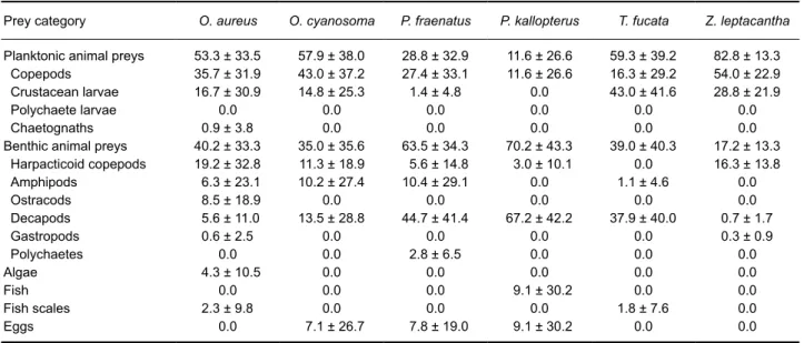
Table 3. Mean percent composition of all dietary categories in the six species of apogonids collected in
2014. Results are presented as Mean (%) ± SD. O. = Ostorhinchus, P. = Pristiapogon, T. = Taeniamia, Z. =
Zoramia
Prey category O. aureus O. cyanosoma P. fraenatus P. kallopterus T. fucata Z. leptacantha Planktonic animal preys 53.3 ± 33.5 57.9 ± 38.0 28.8 ± 32.9 11.6 ± 26.6 59.3 ± 39.2 82.8 ± 13.3
Copepods 35.7 ± 31.9 43.0 ± 37.2 27.4 ± 33.1 11.6 ± 26.6 16.3 ± 29.2 54.0 ± 22.9 Crustacean larvae 16.7 ± 30.9 14.8 ± 25.3 1.4 ± 4.8 0.0 43.0 ± 41.6 28.8 ± 21.9
Polychaete larvae 0.0 0.0 0.0 0.0 0.0 0.0
Chaetognaths 0.9 ± 3.8 0.0 0.0 0.0 0.0 0.0
Benthic animal preys 40.2 ± 33.3 35.0 ± 35.6 63.5 ± 34.3 70.2 ± 43.3 39.0 ± 40.3 17.2 ± 13.3 Harpacticoid copepods 19.2 ± 32.8 11.3 ± 18.9 5.6 ± 14.8 3.0 ± 10.1 0.0 16.3 ± 13.8 Amphipods 6.3 ± 23.1 10.2 ± 27.4 10.4 ± 29.1 0.0 1.1 ± 4.6 0.0 Ostracods 8.5 ± 18.9 0.0 0.0 0.0 0.0 0.0 Decapods 5.6 ± 11.0 13.5 ± 28.8 44.7 ± 41.4 67.2 ± 42.2 37.9 ± 40.0 0.7 ± 1.7 Gastropods 0.6 ± 2.5 0.0 0.0 0.0 0.0 0.3 ± 0.9 Polychaetes 0.0 0.0 2.8 ± 6.5 0.0 0.0 0.0 Algae 4.3 ± 10.5 0.0 0.0 0.0 0.0 0.0 Fish 0.0 0.0 0.0 9.1 ± 30.2 0.0 0.0 Fish scales 2.3 ± 9.8 0.0 0.0 0.0 1.8 ± 7.6 0.0 Eggs 0.0 7.1 ± 26.7 7.8 ± 19.0 9.1 ± 30.2 0.0 0.0
benthic compartment than P. kallopterus and P.
fraenatus (Tables 3 and 4). No significant variation
was shown for the other species (Table 4).
Stable isotopes
Zooplankton δ13C was comparable in 2011
and 2012, but less negative in 2014 (Fig. 1A). Carbon isotopic composition of zoobenthos was variable according to sampling year (Fig. 1A), but it was more 13C-enriched than zooplankton in both
2011 and 2014. The difference between mean δ13C
of the two food items varied drastically according to sampling year, as it was 5.73‰ in 2011 but only 0.97‰ in 2014. δ15N of food items did not seem to
follow a consistent temporal variation pattern, and was quite comparable for both food items in every sampling year (Fig. 1A).
Carbon isotopic composition of cardinalfishes was spread over a large interval (Fig. 1A), with values ranging from -11.14 ± 0.45‰ (Ostorhinchus
cookii in 2011; mean ± SD) to -16.97 ± 0.37‰
(Taeniamia fucata in 2014; mean ± SD). Nitrogen isotopic composition also showed considerable dispersion (Fig. 1A), as values ranged from 6.61 ± 0.19‰ (O. cookii in 2011; mean ± SD) to 10.14 ± 0.61‰ (P. kallopterus in 2014; mean ± SD). This isotopic variability was partly related to the sampling year, as δ13C and δ15N seemed to
shift towards more negative and higher values throughout time, respectively. However, species-specific trends were also present. For example, δ15N of P. kallopterus and P. fraenatus were
identical in 2011 (Mann-Whitney test: U = 19,
P = 0.113; Fig. 1A), but P. kallopterus showed
significantly higher δ15N than P. fraenatus in 2014
(Mann-Whitney test: U = 72.5, P < 0.001; Fig. 1A). In 2011, δ13C of fishes showed significant
interspecific variation (Kruskal-Wallis test: H = 34.12, P < 0.001). Post-hoc multiple comparisons
(Dunn’s test) showed that two groups were present (Fig. 1A): one composed of P. fraenatus and O.
cookii, and another composed of P. kallopterus
and O. cyanosoma. The latter group had more negative δ13C than the former, suggesting that, in
2011, zooplankton was more important in the diet of P. kallopterus and O. cyanosoma than in the diet of P. fraenatus and O. cookii. In 2014, significant variation in δ13C was also present (Kruskal-Wallis
test: H = 109.9, P < 0.001). Three groups were present (Dunn’s multiple comparison tests: P < 0.05 in each case): one composed of both species of Pristiapogon (P. fraenatus and P. kallopterus), one composed of both species of Ostorhinchus (O. cookii and O. aureus), and one composed of T. fucata and Z. leptacantha (Fig. 1A). δ13C
decreased, and contribution of zooplankton to diet therefore presumably increased, when going from the first to the third group (Fig. 1A).
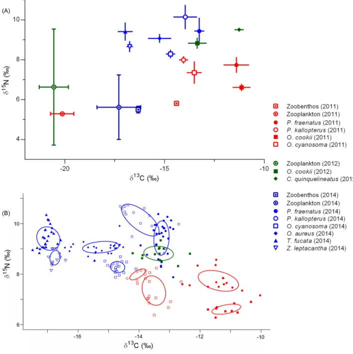
Bivariate standard ellipses of all fish groups were markedly separated (Fig. 1B). This suggests that all cardinalfishes occupy distinct isotopic niches. The only niche overlap found was between
P. fraenatus and P. kallopterus in 2014, and it was
very small (0.04‰2, i.e. 8.46% of the SEAC of P. fraenatus and 5.05% of the SEAC of P. kallopterus;
Fig. 1B). Moreover, there was no overlap between standard ellipses associated with different years for fishes sampled in more than one period (O. cookii, O. cyanosoma, P. fraenatus and P.
kallopterus; Fig. 1B). Isotopic niche width was quite
variable, with SEAC values ranging from 0.13‰2
(P. kallopterus in 2011) to 0.89‰2 (P. kallopterus
in 2014; Fig. 2). Pairwise comparisons of model-estimated ellipse areas (SEAB) suggested niche
width differences among species were robust, as many relative probabilities exceeded 95% (Table 5). Trends for species sampled in successive years were not consistent. Standard ellipse area of P.
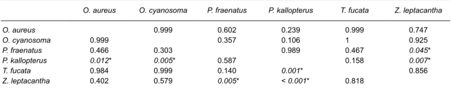
kallopterus showed a drastic increase from 2011 Table 4. Results from Tukey multiple comparisons tests when using data on planktonic (below the diagonal)
and benthic animal preys (above the diagonal). Significant results are highlighted in italics and marked with an asterisk. O. = Ostorhinchus, P. = Pristiapogon, T. = Taeniamia, Z. = Zoramia
O. aureus O. cyanosoma P. fraenatus P. kallopterus T. fucata Z. leptacantha
O. aureus 0.999 0.602 0.239 0.999 0.747 O. cyanosoma 0.999 0.357 0.106 1 0.925 P. fraenatus 0.466 0.303 0.989 0.467 0.045* P. kallopterus 0.012* 0.005* 0.587 0.158 0.007* T. fucata 0.984 0.999 0.140 0.001* 0.856 Z. leptacantha 0.402 0.579 0.005* < 0.001* 0.818
to 2014 (SEAB, 2011 < SEAB, 2014 in 99.94% of model
solutions; Fig. 2 and Table 5). On the other hand, the isotopic niche of O. cyanosoma showed a width decrease from 2011 to 2014 (SEAB, 2014 < SEAB, 2011
in 100% of model solutions; Fig. 2 and Table 5). Probabilities of standard ellipse area differences in
O. cookii (SEAB, 2011 < SEAB, 2012 in 87.58% of model
solutions) and P. fraenatus (SEAB, 2011 < SEAB, 2014
in 11.21% of model solutions; Fig. 2 and Table 5) were inferior to 95%, suggesting no meaningful temporal trend in niche width in these taxa. Finally, there was no relation between SEAC and the
size range of sampled fishes (linear regression analysis, R2 = 0.15, P = 0.24), suggesting that the
Fig. 1. (A) Mean values (± SD) of δ13C (‰) and δ15N (‰) of cardinalfishes. (B) Isotopic niches of cardinalfishes. Points are individual
measurements, and solid lines represent the bivariate standard ellipses associated to each group Species and sampling years are represented by different symbols and colors, respectively.
(A)
isotopic niche size was not related to variation in size ranges of the studied species (Table 1).
Linear regression analyses revealed that the variation of carbon or nitrogen isotopic compositions was size-related in most of the apogonids (0.22 ≤ R2 ≤ 0.90; Fig. 3). However, size
range varied greatly among species samples (Table
1) and that could have impacted the results of linear models. For example, Z. leptacantha was the only species for which the isotopic compositions were unexplained by body size but its size range was the smallest from all studied species (size range = 5.5 mm; Table 1). In P. fraenatus, P.
kallopterus and T. fucata, there was a strong,
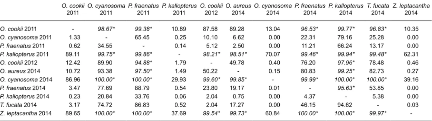
Table 5. Pairwise comparisons of standard ellipses areas of cardinalfishes estimated through Bayesian
modeling (SEAB). Each cell contains the relative probability (%) that the standard ellipse of the fish group
listed as line is smaller than the standard ellipse of the fish group listed as column, based on 106 model
runs. Values highlighted in italics and marked with an asterisk are probabilities higher than 95%. O. =
Ostorhinchus, P. = Pristiapogon, T. = Taeniamia, Z. = Zoramia
O. cookii
2011 O. cyanosoma2011 P. fraenatus 2011 P. kallopterus 2011 O. cookii 2012 O. aureus2014 O. cyanosoma 2014 P. fraenatus 2014 P. kallopterus2014 T. fucata 2014 Z. leptacantha2014
O. cookii 2011 - 98.67* 99.38* 10.89 87.58 89.28 13.04 96.53* 99.77* 96.83* 10.35 O. cyanosoma 2011 1.33 - 65.45 0.25 10.10 6.62 0.00 22.31 79.16 25.28 0.00 P. fraenatus 2011 0.62 34.55 - 0.14 5.12 2.50 0.00 11.21 66.24 13.17 0.00 P. kallopterus 2011 89.11 99.75* 99.86* - 98.21* 98.51* 70.07 99.46* 99.94* 99.48* 62.31 O. cookii 2012 12.42 89.90 94.88* 1.79 - 49.78 0.40 76.20 97.96* 78.48 0.46 O. aureus 2014 10.72 93.38 97.50* 1.49 50.22 - 0.15 80.83 99.25* 82.73 0.27 O. cyanosoma 2014 86.96 100.00* 100.00* 29.93 99.60* 99.85* - 99.99* 100.00* 100.00* 39.16 P. fraenatus 2014 3.47 77.69 88.79 0.54 23.80 19.17 0.01 - 95.63* 53.85 0.00 P. kallopterus 2014 0.23 20.84 33.76 0.06 2.04 0.75 0.00 4.37 - 5.38 0.00 T. fucata 2014 3.17 74.72 86.83 0.52 2.04 17.27 0.00 46.15 94.62 - 0.03 Z. leptacantha 2014 89.65 100.00* 100.00* 37.69 99.54* 99.73* 60.84 100.00* 100.00* 99.97*
-Fig. 2. Boxplots of model-estimated bivariate standard ellipse area (SEAB). Dark, median and light grey boxes are respectively the
50%, 75% and 95% credibility intervals of the probability of density function distributions of the model solutions, and black dots are the modes of these distributions. Red dots represent the standard ellipse areas computed using a frequentist algorithm adapted for small sample sizes (SEAC).
Fig. 3. Relationship between body size (SL, mm) and isotopic values (A: δ13C; B: δ15N) in studied apogonids. Only significant
relationships are illustrated.
48 54 60 66 -12.0 -11.5 -11.0 -10.5 37.5 40.0 42.5 45.0 -14.0 -13.6 -13.2 -12.8 42.5 45.0 47.5 50.0 -15.00 -14.75 -14.50 -14.25 44 48 52 56 -14.4 -14.2 -14.0 -13.8 64 72 80 88 -14.5 -14.0 -13.5 -13.0 (A) (B) 50 60 70 80 90 8.4 8.8 9.2 9.6 48 56 64 72 6.25 6.50 6.75 7.00 36 39 42 45 48 6.6 7.2 7.8 8.4 60 70 80 90 7.2 8.0 8.8 9.6 10.4 60 70 80 90 8.4 9.0 9.6 10.2 10.8 64 68 72 76 8.4 9.0 9.6 10.2 R2 = 0.61 P = 0.01 R 2= 0.32 P = 0.03 R 2 = 0.22 P = 0.04 R2 = 0.83 P = 0.04 R 2 = 0.44 P = 0.006 R2 = 0.31 P = 0.004 R2 = 0.69 P = 0.008 P = 0.04 R2 = 0.86 P = 0.0001 R 2 = 0.90 P = 0.0001 R 2 = 0.46 P = 0.001 δ 15N δ 15N δ 15N δ 15N δ 15N δ 15N R2 = 0.29 δ 13C δ 13C δ 13C δ 13C δ 13C
O. cookii (2011) O. cyanosoma (2011) O. cyanosoma (2014)
SL (mm)
P. kallopterus (2011) P. kallopterus (2014)
O. aureus (2014) O. cookii (2011) O. cyanosoma (2011)
P. fraenatus (2014) P. kallopterus (2014) T. fucata (2014)
SL (mm) SL (mm) SL (mm) SL (mm) SL (mm) SL (mm) SL (mm) SL (mm) SL (mm) SL (mm)
significant positive relationship between fish size and δ15N (Fig. 3). Possibilities of comparisons
between sampling years were limited but, in P.
kallopterus, the positive relationship between
fish size and δ13C observed in 2011 shifted to a
negative one in 2014 (Fig. 3). In the great majority of species, the δ13C and the δ15N values were
unrelated to the proportion of zooplankton found in stomach contents (Linear regressions: R2 ≤ 0.21, P > 0.05; data not shown). Only in P. kallopterus
from 2014 was the percentage of zooplankton slightly related to δ13C values (R2 = 0.37, P = 0.04).
DISCUSSION
Stomach content analyses show that cardinalfishes from Toliara lagoon have somehow similar carnivorous diets. On the other hand, the stable isotope analyses provide some evidences for fine-scale niche partitioning in apogonids, because no overlap among species was observed in the isotopic space. Size-related variation in stable isotope composition of fishes also suggests niche partitioning within some species.
Both stomach contents and isotope data show that cardinalfishes feed on planktonic and benthic animal prey in various proportions, which is in agreement with previous studies (Vivien 1975; Marnane and Bellwood 2002; Barnett et al. 2006). Except some small fishes encountered in the stomachs of Pristiapogon kallopterus, we found low evidence of piscivory in the studied species. Vivien (1975) was able to delineate three trophic groups: strict planktivorous species, strict benthic feeders, and species eating both types of animal prey. This discrimination is not obvious in the present study and we argue in favor of generalist, carnivorous diets in cardinalfishes with some feeding preferences (see also Marnane and Bellwood 2002; Barnett et al. 2006). For example, stable isotope ratios suggest that Pristiapogon
fraenatus and P. kallopterus mainly forage on
benthic prey but zooplankton or even small fishes were found in their stomachs (Fig. 1A; Table 2).
Large intra-specific variation in the stomach contents (Table 3) and temporal variation in the relative contribution of prey to diet (Fig. 1) are further arguments to characterize the feeding ecology of apogonids as generalist, carnivorous fishes. To date, relatively few studies have illustrated temporal variation in the diet of coral reef fishes and most of them focused on diurnal fishes (e.g. Letourneur et al. 1997; Frédérich et
al. 2016). Stomach contents provide information on the most recent meal only, making this method much more sensitive to temporal variation (Hyslop 1980). Here, frequency of occurrence of dietary categories suggested that Ostorhinchus cookii consumed a larger proportion of planktonic prey in 2012 than in 2011. This trend was confirmed by isotopic compositions, revealing that this variation in feeding habits might persist for longer periods. At the Great Reef of Toliara (GRT), Vivien (1975) classified Ostorhinchus cyanosoma as a zooplankton specialist while Marnane and Bellwood (2002) found that zoobenthos may account for a large proportion of its diet at One Tree Island (Australia). Our data suggest that, at the Toliara Reef, O. cyanosoma has a mixed diet (e.g. intermediate δ13C values in 2014; Fig. 1A)
and feeds on both zoobenthos and zooplankton. The diet of apogonids may vary at smaller spatial scales. Indeed, Vivien (1975) illustrated considerable variations in the diet of Ostorhinchus
endekataenia and P. kallopterus living in different
biotopes from the GRT. For example, P. kallopterus ingests a large proportion of isopods in seagrass beds when it feeds largely on shrimps on the reef slopes (Vivien 1975). All these examples of temporal and spatial variation in the feeding preferences clearly demonstrate opportunism and diet plasticity in cardinalfishes.
Nevertheless, the present study is the first, to our knowledge, that illustrates a segregation of isotopic niches in an assemblage of cardinalfishes. For each sampling year, fish δ13C values were
scattered over a ~4‰ range. Carbon stable isotope ratios are mostly influenced by consumer preferences in prey type or foraging habitat. Indeed, as illustrated in previous studies on the trophic ecology of damselfishes from the GRT (Frédérich et al. 2009, 2010; Lepoint et al. 2016), the δ13C axis represents a continuum of food
sources from plankton (the most negative values) to zoobenthos (the least negative values; Fig. 1A). Differences in the C isotopic values were also demonstrated for fish species living in different areas (Frédérich et al. 2012; Letourneur et al. 2013) or different micro-habitats (Lepoint et al. 2016) of the same coral reef. δ15N is well known
for showing a stepwise increase with increasing trophic level (DeNiro and Epstein 1981) and this second niche axis is therefore related to trophic position. Here, δ15N values varied within a
~2-3‰ interval among apogonids of each sampling year. As evidenced by the lack of overlap of standard ellipses (Fig. 1B), all the cardinalfish
species showed distinct isotopic niches that differ by at least one of the two niche axes. This suggests ecological niche segregation within the assemblage. Differences in these isotopic niches may be related to different diet (i.e. varied prey species) but also to different trophic behavior (e.g. pelagic vs. benthic), different foraging habitat (e.g. water column, coral boulders, sandy areas) or different foraging location in the same habitat, as stable isotope composition may vary spatially. Relatively high similarity in the composition of stomach contents among species (Tables 2 and 3) does not support that the variation in isotopic niches is mainly related to strong short-term differences in the type of prey selected. Nevertheless, we cannot reject the possibility that an analysis of stomach contents with higher resolution (i.e. identification of prey to lower taxonomic levels – e.g. family or species) could help to refine such an assumption. On the other hand, we argue that differences in isotopic niches reflect a partitioning of foraging locations and/or behaviors among species. Indeed, isotopic niche variability is also determined by isotopic variability of sources (so-called baseline shifts; Boecklen et al. 2011), that could in turn be related to spatial variability (Flaherty and Ben-David 2010). Thus, species differ significantly in their isotopic niches because the isotopic composition of their food sources differs spatially. This hypothesis is in total agreement with the visual surveys of Marnane and Bellwood (2002) revealing that different apogonid species share restricted resting habitats by day but they segregate spatially at night, both horizontally and vertically in the water column. By reporting different foraging locations in six species of Hawaiian cardinalfishes at night, the observations of Chave (1978) strengthen our statement. Thus, apogonids may forage in the water column, over horizontal substrates, over vertical substrates or near holes in isolated coral heads. In the same habitat, apogonids may segregate spatially, feeding on the same food resource but in various places.
The ecological niche (sensu Hutchinson 1957) of a species is defined as a n-dimensional hypervolume whose axes represent environmental and/or resource requirements of this organism. The isotopic niche must be seen as a proxy of this ecological niche, integrating two of its axes subsets, i.e. both trophic and habitat-related information (Flaherty and Ben-David 2010). Here, isotopic niche width (i.e. standard ellipse area) was quite variable among species and also varied
temporally. No major interspecific differences in stomach content compositions of apogonids suggest that the breadth of isotopic niches could be more related to the diversity of foraging locations (i.e. microhabitat segregation) than to diversity of consumed prey species. Species showing small standard ellipse areas (e.g. Z.
leptacantha and O. cyanosoma [2014]) could be
considered as specialists in their foraging areas, when others are feeding on prey dispersed on various locations (e.g. T. fucata, P. fraenatus, P.
kallopterus). Although there were considerable
differences in the size ranges of sampled fishes for each species, the lack of relation between size ranges and standard ellipse areas suggest that potential sampling biases related to fish size are unlikely.
Hutchinson (1957) distinguished the funda-mental and realized ecological niches. The fundamental niche of a species may be assessed when the effects of biotic interactions (competition and predation) are excluded. Conversely, the realized niche is obtained when the biotic interactions are included in the calculation of the niche. The realized niche is typically a smaller volume than the fundamental region within a multidimensional hyperspace (Kearney 2006). The fundamental trophic niche of most cardinalfishes is a carnivorous diet made of small pelagic and benthic animal prey. The niche differentiation in the isotopic space conceptualizes their realized niche. Segregation is likely to operate through a combination of different factors, including morphological, physiological and behavioral adaptations. To date, ecomorphological studies did not find morphological traits explaining dietary segregation in apogonids (Barnett et al. 2006) but behavioral adaptations might certainly support it (Chave 1978; Marnane and Bellwood 2002). Our temporal datasets demonstrate that the realized trophic niche of cardinalfishes is dynamic both spatially and temporally, and contextualized. Indeed, the relative position of every species in the isotopic space varied across time and sampled populations. For example, in 2011, P. kallopterus was significantly more 13C-depleted than P. fraenatus, while in 2014 the two species showed
statistically identical δ13C values. Conversely, the
δ15N of these two species were identical in 2011,
but different in 2014 (Fig. 1A). In addition, the isotopic niche width of one species may greatly vary between two time periods. Accordingly, O.
cyanosoma showed one of the smallest standard
alongside P. fraenatus in 2011. Inter-specific and inter-guild competition, food abundance and habitat structural complexity are probably main factors shaping resource segregation and associated feeding ecology of cardinalfishes on the Great Reef of Toliara.
The majority of studied apogonids showed size-related variation of isotopic compositions. These relationships may be interpreted as diet shift (Frédérich et al. 2010), habitat shift (Frédérich et al. 2012) or temporal variability of food sources (Matthews and Mazumder 2005). Linear models revealed that the variation in isotopic compositions is often poorly related to diet changes in the type of prey but we argue that the variation of δ15N
could be at least related to changes in the size of prey (Frédérich et al. 2010). Size-variation of the isotopic values could be an evidence of some partitioning in foraging locations among individuals of the same species. On the other hand, we also need to be cautious about the ecological interpretation of these variations. In some species, the isotopic compositions varied less than 1-1.5‰ across body size range (e.g. O. cookii 2011, O.
cyanosoma 2014, P. kallopterus 2011; Fig. 3)
and such variation could be influenced by age-related variability in diet-tissue fractionation and/or physiology (Sweeting et al. 2007a, b; Gajdzik et al. 2015).
To conclude, the present study provides some evidence of niche partitioning in an assemblage of Apogonidae. All species feed on small benthic and planktonic animal prey in variable proportions but the isotopic data suggest a segregation of their foraging locations. The trophic niche partitioning among cardinalfishes is dynamic, changing across time and it is shaped by various factors determining a niche segregation context. Further studies are needed to explore the drivers of feeding ecology in Apogonidae and to question the redundancy of their functional roles in coral reef ecosystems.
Acknowledgments: Authors wish to thank the
staff of the Institut Halieutique et des Sciences Marines (IH.SM) of Toliara for their welcome and their logistical help. Prof. Igor Eeckhaut is also acknowledged for giving us the opportunity to use BIOMAR facilities. We also warmly thank Pierre Vandewalle and our Vezo crew captain Noëlson for help during field works. B.F. and L.N.M. are BELSPO (Belgian Federal Science Policy Office) post-doctoral fellows. G.L. is a Research Associate from the “Fonds National de la Recherche
Scientifique of Belgium” (F.R.S-FNRS). Field campaigns on the Great Reef of Toliara were funded by the “Agathon De Potter” funds from the Royal Academy for Sciences of Belgium and F.R.S.-FNRS travel grants (“short stay abroad” grants nr. 2014/V3/5/233 and 2014/V3/5/234).
REFERENCES
Annese DM, Kingsford MJ. 2005. Distribution, movements and diet of nocturnal fishes on temperate reefs. Environ Biol Fishes 72(2):161-174. doi:10.1007/s10641-004-0774-7.
Barnett A, Bellwood DR, Hoey AS. 2006. Trophic ecomorphology of cardinalfish. Mar Ecol Prog Ser
322:249-257. doi:10.3354/meps322249.
Bearhop S, Adams CE, Waldron S, Fuller RA, Macleod H. 2004. Determining trophic niche width: a novel approach using stable isotope analysis. J Anim Ecol
73(5):1007-1012. doi:10.1111/j.0021-8790.2004.00861.x.
Boecklen WJ, Yarnes CT, Cook BA, James AC. 2011. On the use of stable isotopes in trophic ecology. Annu Rev Ecol Evol Syst 42:411-440.
doi:10.1146/annurev-ecol-sys-102209-144726.
Chave EH. 1978. General ecology of six species of Hawaiian cardinalfishes. Pac Sci 32(3):245-270.
Clarke KR, Warwick RM. 2001. Change in marine communities: an approach to statistical analysis and interpretation. PRIMER-E, Plymouth, UK.
Coplen TB. 2011. Guidelines and recommended terms for expression of stable-isotope-ratio and gas-ratio measurement results. Rapid Commun Mass Spectrom
25:2538-2560. doi:10.1002/rcm.5129.
DeNiro MJ, Epstein S. 1981. Influence of diet on the distribution of nitrogen isotopes in animals. Geochim Cosmochim Acta 45(3):341-351.
doi:https://doi.org/10.1016/0016-7037(81)90244-1.
Eschmeyer WN, Fricke R, van der Laan R. 2016. Catalog of fishes. http://research.calacademy.org/research/ ichthyology/catalog/fishcatmain.asp Accessed 15 July 2016.
Flaherty EA, Ben-David M. 2010. Overlap and partitioning of the ecological and isotopic niches. Oikos
119(9):1409-1416. doi:10.1111/j.1600-0706.2010.18259.x.
Frédérich B, Colleye O, Lepoint G, Lecchini D. 2012. Mismatch between shape changes and ecological shifts during the post-settlement growth of the surgeonfish, Acanthurus triostegus. Front Zool 9:8. doi:10.1186/1742-9994-9-8.
Frédérich B, Fabri G, Lepoint G, Vandewalle P, Parmentier E. 2009. Trophic niches of thirteen damselfishes (Pomacentridae) at the Grand Récif of Toliara, Madagascar. Ichthyol Res 56(1):10-17. doi:10.1007/
s10228-008-0053-2.
Frédérich B, Lehanse O, Vandewalle P, Lepoint G. 2010. Trophic Niche Width, Shift, and Specialization of Dascyllus aruanus in Toliara Lagoon, Madagascar. Copeia
2010(2):218-226.
doi:http://dx.doi.org/10.1643/CE-09-031.
Frédérich B, Olivier D, Gajdzik L, Parmentier E. 2016. Trophic ecology of damselfishes. In: Frédérich B, Parmentier E (eds) Biology of Damselfishes. CRC Press, Boca Raton, pp. 153-167.
Gajdzik L, Lepoint G, Lecchini D, Frédérich B. 2015. Comparison of isotopic turnover dynamics in two different muscles of a coral reef fish during the settlement phase. Sci Mar 79(3):325-333. doi: http://dx.doi.org/10.3989/
scimar.04225.31A.
Gladfelter WB, Johnson WS. 1983. Feeding niche separation in a guild of tropical reef fishes (Holocentridae). Ecology
64(3):552-563. doi:10.2307/1939975.
Hammer O, Harper DAT, Ryan PD. 2001. PAST: Paleontological Statistics software package for education and data analysis. Palaeontol Electron 4:1-9.
Harmelin-Vivien M. 2002. Energetics and fish diversity on coral reefs. In: Sale PF (ed) Coral reef fishes Dynamics and diversity in a complex ecosystem Academic Press, Boston, pp. 265-274.
Hobson ES. 1965. Diurnal-nocturnal activity of some inshore fishes in the Gulf of California. Copeia 1965(3):291-302.
doi:10.2307/1440790.
Hobson ES. 1972. Activity of Hawaiian reef fishes during the evening and during transition between daylight and darkness. Fish Bull 70:715-740.
Hutchinson GE. 1957. Concluding remarks. Cold Spring Harbor Symp 22:415-427.
Hyslop EJ. 1980. Stomach contents analysis – a review of methods and their application. J Fish Biol 17:411-429.
doi:10.1111/j.1095-8649.1980.tb02775.x.
Jackson AL, Inger R, Parnell AC, Bearhop S. 2011. Comparing isotopic niche widths among and within communities: SIBER - Stable Isotope Bayesian Ellipses in R. J Anim Ecol 80(3):595-602. doi:10.1111/j.1365-2656.2011.01806.
x.
Kearney M. 2006. Habitat, environment and niche: What are we modelling? Oikos 115(1):186-191. doi:10.1111/
j.2006.0030-1299.14908.x.
Layman CA, Allgeier JE. 2012. Characterizing trophic ecology of generalist consumers: a case study of the invasive lionfish in The Bahamas. Mar Ecol Prog Ser 448:131-141.
doi:https://doi.org/10.3354/meps09511.
Layman CA, Araujo MS, Boucek R, Hammerschlag-Peyer CM, Harrison E, Jud ZR, Matich P, Rosenblatt AE, Vaudo JJ, Yeager LA, Post DM, Bearhop S. 2012. Applying stable isotopes to examine food-web structure: An overview of analytical tools. Biol Rev 87(3):545-562. doi:10.1111/
j.1469-185X.2011.00208.x.
Lepoint G, Michel LN, Parmentier E, Frédérich B. 2016. Trophic ecology of the seagrass-inhabiting footballer demoiselle Chrysiptera annulata (Peters, 1855); comparison with three other reef-associated damselfishes. Belg J Zool
146(1):21-32.
Letourneur Y, Galzin R, Harmelin-Vivien M. 1997. Temporal variations in the diet of the damselfish Stegastes nigricans
(Lacepede) on a Reunion fringing reef. J Exp Mar Biol Ecol 217(1):1-18.
doi:https://doi.org/10.1016/S0022-0981(96)02730-X.
Letourneur Y, Lison de Loma T, Richard P, Harmelin-Vivien ML, Cresson P, Banaru D, Fontaine MF, Gref T, Planes S. 2013. Identifying carbon sources and trophic position of coral reef fishes using diet and stable isotope (δ15N and δ13C) analyses in two contrasted bays in Moorea, French Polynesia. Coral Reefs 32(4):1091-1102. doi:10.1007/
s00338-013-1073-6.
Marnane MJ, Bellwood DR. 2002. Diet and nocturnal foraging in cardinalfishes (Apogonidae) at One Tree Reef, Great Barrier Reef, Australia. Mar Ecol Prog Ser 231:261-268.
Matthews B, Mazumder A. 2005. Consequences of large temporal variability of zooplankton δ15N for modeling fish trophic position and variation. Limnol Oceanogr
50(5):1404-1414.
Michel L, Lepoint G, Dauby P, Sturaro N. 2010. Sampling methods for amphipods of Posidonia oceanica meadows: A comparative study. Crustaceana 83(1):39-47.
doi:10.1163/156854009X454630.
Peterson BJ, Fry B. 1987. Stable isotopes in ecosystem studies. Annu Rev Ecol Syst 18:293-320. doi:10.1146/
annurev.es.18.110187.001453.
Pratchett MS. 2005. Dietary overlap among coral-feeding butterflyfishes (Chaetodontidae) at Lizard Island, northern Great Barrier Reef. Mar Biol 148(2):373-382. doi:10.1007/
s00227-005-0084-4.
R Development Core Team. 2015. R: A language and environment for statistical computing. Vienna, Austria. http://www.R-project.org.
Randall JE. 1967. Food habits of reef fishes of the West Indies. Studies in Tropical Oceanography 5:665-847.
Schoener TW. 1974. Resource partitioning in ecological communities. Science 185:27-39. doi:10.1126/
science.185.4145.27.
Sweeting CJ, Barry J, Barnes C, Polunin NVC, Jennings S. 2007a. Effects of body size and environment on diet-tissue δ15N fractionation in fishes. J Exp Mar Biol Ecol
340(1):1-10. doi:http://doi.org/340(1):1-10.1016/j.jembe.2006.07.023. Sweeting CJ, Barry JT, Polunin NVC, Jennings S. 2007b.
Effects of body size and environment on diet-tissue δ13C fractionation in fishes. J Exp Mar Biol Ecol
352(1):165-176. doi:http://doi.org/10.1016/j.jembe.2007.07.007. Vivien ML. 1975. Place of apogonid fish in the food webs of a
Malagasy coral reef. Micronesica 11(2):185-196.
Wainwright PC, Bellwood DR. 2002. Ecomorphology of feeding in coral reef fishes. In: Sale PF (ed) Coral reef fishes: dynamics and diversity in a complex ecosystem. Academic Press, San Diego, pp. 33-56.
Supplementary Material
Table S1. Isotopic compositions of food sources.