A Supervised Machine Learning Approach to
Variable Branching in Branch-And-Bound
Alejandro Marcos Alvarez, Quentin Louveaux, and Louis Wehenkel⋆
Universit´e de Li`ege, Department of EE&CS, Sart-Tilman B28, Li`ege, Belgium {amarcos,q.louveaux,l.wehenkel}@ulg.ac.be
Abstract. We present in this paper a new approach that uses supervised machine learning techniques to improve the performances of optimization algorithms in the context of mixed-integer programming (MIP). We fo-cus on the branch-and-bound (B&B) algorithm, which is the traditional algorithm used to solve MIP problems. In B&B, variable branching is the key component that most conditions the efficiency of the optimization. Good branching strategies exist but are computationally expensive and usually hinder the optimization rather than improving it. Our approach consists in imitating the decisions taken by a supposedly good branching strategy, strong branching in our case, with a fast approximation. To this end, we develop a set of features describing the state of the ongoing optimization and show how supervised machine learning can be used to approximate the desired branching strategy. The approximated function is created by a supervised machine learning algorithm from a set of ob-served branching decisions taken by the target strategy. The experiments performed on randomly generated and standard benchmark (MIPLIB) problems show promising results.
Keywords: branch-and-bound, variable branching, supervised learning
1
Introduction
Mixed-Integer Programming (MIP) problems are optimization problems in which some, or all, of the variables can only take integral values. This type of prob-lems is ubiquitous in many areas such as operations research and power systems. Scheduling [8], shortest path finding [23] and power systems security manage-ment [16] are some typical applications modeled in the form of MIP problems.
Most MIP solvers are based on the branch-and-bound (B&B) algorithm [18]. B&B constructs an optimization tree that enumerates only the interesting can-didate solutions. Each node of the tree corresponds to a version of the initial problem in which some integrality constraints on the variables have been relaxed.
⋆This work was funded by the Biomagnet IUAP network of the Belgian Science Policy
Office and the Pascal2 network of excellence of the EC. AMA’s thesis is funded by a FRIA scholarship from the F.R.S.-FNRS. The scientific responsibility rests with the authors.
The optimization tree is built in such a way that each node has one additional integrality constraint, i.e. one variable is forced to an integral value, than its parent node. Therefore, the solutions of the initial problem (respecting all initial integrality constraints) are traditionally found in the deeper nodes. For a given problem, there exist many possible optimization trees, of different sizes, because there are usually several possible integrality constraints that can be added to one node to create its children. A branching strategy is a function that arbitrates between those possible choices with the goal of yielding a tree that is as small as possible.
Over the years, numerous fundamental features, such as cutting planes, pre-solve, heuristics or advanced branching strategies, have been added to the solvers in order to improve their performances [4]. However, among those additional fea-tures, branching, i.e. the process that divides the feasible region into two or more subproblems, is probably the key component that most conditions the efficiency of a solver [4].
Different branching strategies create different optimization trees, of different sizes, and a good branching strategy is typically designed such that the number of nodes of the tree that it induces is as small as possible. However, taking branching decisions that minimize the total number of explored nodes is usually time consuming. Accordingly, branching strategies need to find a good tradeoff between the time spent to take a decision and the overall optimization time that is directly influenced by the number of explored nodes. One of the most effective strategy in terms of the size of the optimization tree is known as strong branching. This heuristic is however very time consuming and therefore unusable in practice.
Our goal is to overcome the large computational overhead resulting from a strong branching decision, while keeping the size of the tree as small as possible. Speeding up strong branching-like decisions is not a new idea, as it is already be-hind other branching heuristics such as reliability branching [2] or non-chimerical branching [13]. In this paper, we propose an alternative approach that uses ma-chine learning techniques to imitate the strong branching decisions in an efficient way. More specifically, we propose a two-phased approach that yields a ‘learned’ branching strategy that can be used within B&B as an approximation of strong branching. The first phase consists in optimizing a set of training problems with strong branching as branching heuristic in order to generate a set of branching decisions. During this phase, each branching decision is recorded in a learning set that will then be used by a supervised machine learning algorithm to learn a function imitating strong branching decisions. In the second phase, we introduce, as any other branching heuristic, the learned heuristic into B&B, and evaluate its efficiency on a set of standard benchmark problems, the MIPLIB [3,9]. Although the performances of the learned branching strategy are still a little below state-of-the art methods, the results show that our approach succeeds in efficiently approximating strong branching decisions.
The idea of observing past branching decisions in order to improve the branching choices made by B&B has already received some attention in the
integer programming literature [12,17]. The main differences between our ap-proach and previous work are that, in this paper, the ‘learning’ phase is done in an off-line fashion and that we use a ‘real’ machine learning algorithm. Indeed, once the branching heuristic is learned from the learning set with a learning algorithm, the learned heuristic can be included directly into B&B, without re-quiring a new learning phase each time a problem needs to be solved. This stands in contrast with other ‘learning-based’ approaches to variable branching [12,17] that require for each problem to solve a new time-consuming ‘learning’ phase.
2
Preliminaries
In this paper, we address binary Mixed-Integer Linear Programming (MILP) problems of the form
min c⊤
x (1)
s.t. Ax ≤ b
xj ∈ {0, 1} ∀j ∈ I
xj ∈ R+∀j ∈ C,
where c ∈ Rn, A ∈ Rm×n and b ∈ Rmrespectively denote the cost coefficients,
the coefficient matrix and the right-hand side. I and C are two sets containing the indices of the integer and continuous variables respectively. We denote the solution at a given node of the B&B by x∗ and we will call, with a little abuse,
the variable xi, with i ∈ I, a fractional variable if it has a fractional value in
the current solution x∗. The set of fractional variables of x∗ is denoted F . The
value c⊤x′ is called the objective value of the solution x′.
The branch-and-bound (B&B) algorithm [18] is the traditional approach to solve problems that can be reformulated in the form of (1). For the reader unfamiliar with B&B, we concisely explain in the following its main mechanics in the case of binary MIP problems1.
B&B builds an optimization tree in which each node represents a version of the initial optimization problem where some integrality constraints of the variables in I have been relaxed, i.e. xi ∈ [0, 1] for some i ∈ I. Because some
integrality constraints are relaxed, the problem contained in each node is called a linear programming relaxation (LP-relaxation) of the initial problem, and is solved with a traditional linear programming method, e.g. the simplex [10]. If the solution found at one node, i.e. the solution of one LP-relaxation, violates some of the initial integrality constraints that remain relaxed at the current node, i.e. the set F is non empty, the algorithm creates two nodes, corresponding to two new subproblems. To create them, B&B adds to the current subproblem additional constraints for variable i ∈ F such that these constraints cut, from the current set of feasible solutions, the current value of variable i, i.e. x∗
i ∈ Z./
1
We present the B&B in the case of a minimization problem, but a similar reasoning applies when the problem is a maximization problem.
In the case of binary problems, one subproblem is created by adding to the current subproblem one constraint of the form xi≤ 0 and the other subproblem
is created by the addition of xi≥ 1, such that variable i is forced to an integral
value in the descendants of those nodes. This operation is called branching on variable i. On the other hand, when the solution found at one node respects all initial integrality constraints, i.e. the set F is empty at that node, then the algorithm has found a solution (not necessarily optimal) of the problem and the exploration of that branch of the tree is stopped. The optimization tree is built so that such solutions are found in deeper nodes of the tree. B&B can also decide not to explore one node if the objective value at that node is greater than the objective value of the best (integral) solution found thus far. Once the tree has been entirely explored, the integral solution with the smallest objective value is returned as the optimal solution of the initial problem.
The branching strategy, i.e. the function that chooses a variable i in the set F , is probably the component of B&B that most influences the efficiency of the optimization. Indeed, the branching strategy directly influences the number of nodes that the algorithm has to explore before terminating. This number of nodes has of course to be as small as possible so as to minimize the time required to solve a problem. The most common branching strategies are presented in Section 3.
3
Related work
Branching strategies have been extensively studied in the literature, and we briefly review here some key contributions to that field. The simplest criterion, known as most-infeasible branching, consists in branching on the variable that has the greatest fractional part, i.e. the variable whose fractional part is clos-est to 0.5. However, most-infeasible branching is known to perform poorly in practice and other methods, such as pseudocost branching [6], have later been developed. Pseudocost branching keeps a history of the dual bound increases2
observed during previous branchings, and uses this information to estimate the dual bound improvements for each candidate variable at the current node. Al-though pseudocost branching is very efficient in terms of computation time, the branchings performed at the very beginning of the B&B tree might be inefficient as no reliable history has been recorded at that time. Later, Applegate et al. [5] proposed a strategy, known as strong branching, that overcome this limitation. Strong branching explicitly evaluates the dual bound increase for each fractional variable by actually computing the LP-relaxations resulting from the branching on that variable. The variable that leads to the largest increases is chosen as branching variable for the current node. Despite its apparent simplicity, strong
2
The dual bound refers to the smallest objective value of all open nodes in the op-timization tree. In the context of branching, the dual bound increase refers to the difference between the objective value at the current node and the objective value at one child node. The dual bound increase thus reflects the price one has to pay, in terms of the objective value, to enforce the integrality constraint of a variable.
branching is, up to now, the most efficient branching strategy in terms of the number of B&B nodes. However, this efficiency is achieved at the expense of computation time, and strong branching is unfortunately intractable in prac-tice. More recently, Achterberg et al. [2] proposed to combine the advantages of both pseudocost and strong branching in a branching strategy called reliability branching. Many other branching strategies have been developed for the past 15 years, such as inference branching [19], non-chimerical branching [13], active constraint branching [22] or cloud branching [7], but their thorough description is beyond the scope of this paper. Finally, let us mention hybrid branching [1], which is probably today’s state-of-the-art branching strategy. Hybrid branching efficiently combines five scores obtained from other common branching strate-gies, and is used as the main branching strategy in CPLEX 12.5 [4].
Following the ideas introduced by pseudocost branching, researchers have recently started investigating branching strategies that rely on information col-lected through multiple B&B restarts. Backdoor branching [12] and information-based branching [17] are two key contributions to this aspect. The mechanism of these strategies is two-phased. During the first phase, the optimization of the current problem is restarted from the beginning multiple times, and the algorithm harvests some statistics about each run. In the second phase, the real optimization starts and the harvested information is used to take efficient branching decisions. The idea behind those methods is to quickly and briefly explore different parts of the B&B tree and to decide, based on those shallow explorations, which part it is better to focus on. The work presented in this paper relies on the very same basic idea: explore the search space (in some way or another) and, based on this exploration, quickly decide which branchings are good, and which are not.
Machine learning has already been used to improve optimization algorithms in other contexts. For example, the idea has been applied in the context of SAT solvers to automatically tune the parameters of an algorithm to the instance being solved [15]. Machine learning has also been used to learn search heuristics able to efficiently explore the search space in specific contexts, such as special instances of combinatorial problems [21,24], and protein structure prediction [20]. However, this is the first time, to our knowledge, that machine learning is used in the context of branching in B&B.
4
Problem statement
4.1 Functional form of branching strategies
Any branching heuristic can be formulated in a generic functional form B such that B : (i, ·) 7→ R, where i represents the candidate branching variable, and · represents undefined parameters. The branching variable i∗ is chosen as the one
that maximizes the scores given by B, i.e. i∗= arg max
The functional form B is different for every branching criterion, and proposing a new branching heuristic merely consists in providing a new B, including its implementation and the specification of its arguments.
For example, in the case of most-infeasible branching (MIB), Bmib only
re-quires the current fractional solution to output a score for a variable. Then, the functional form of MIB is written Bmib(i, x∗) = min (x∗i − ⌊x∗i⌋, ⌈x∗i⌉ − x∗i).
An-other example is strong branching (SB), which requires more input arguments as it needs more information to take a decision. The functional form of strong branching is Bsb(i, c, A, b, x∗, l∗, u∗), where l∗and u∗respectively represent the
lower and upper bounds of the variables at the current node. The implementa-tion of Bsb consists in creating two subproblems by changing the upper and
lower bounds of variable i (∈ F ) in the current problem respectively to ⌊x∗ i⌋ and
⌈x∗
i⌉. The LP-relaxations of these subproblems are then solved and, for each
sub-problem, the difference between the objective value of the subproblem and the current problem is computed. These differences represent the objective increases observed between the current node and the subproblems when tighter bounds are used for the variable i. The output of Bsb is finally given by the product of
the computed differences.
4.2 Learning branching decisions
We propose to use machine learning to create a branching heuristic that approx-imates strong branching. In other words, the branching heuristic Blearned(i, φi)
that we suggest is such that
Blearned(i, φi) ≈ Bsb(i, c, A, b, x∗, l∗, u∗) , (2)
where φi is a feature vector describing the state of the optimization problem at
the current node from the perspective of variable i. The feature vector φi does
not describe the current node of the B&B, but rather describes variable i in the current node. Those features need to be computationally efficient and have to well represent the problem at the current B&B node from the perspective of variable i. Section5explains in more details how the features are designed.
In order to apply a supervised machine learning algorithm to create Blearned,
we need a dataset of input-output pairs observed from the function we are trying to approximate. The inputs are given by the features φidescribed in the next
sec-tion and the output is simply the strong branching score Bsb(i, c, A, b, x∗, l∗, u∗).
Once the inputs and the output are specified, a dataset Dsb of strong
branch-ing decisions can be created, before bebranch-ing fed to the learnbranch-ing algorithm. Such a dataset is created by simply recording all the pairs (φi, Bsb(i, ·)) generated for
each fractional variable encountered during the optimization of a set of problems with strong branching as branching strategy.
5
Features describing a variable in the current state of
the problem
The features are the key component of our approach as they critically condition the efficiency of the method. On the one hand, the features need to be complete and precise in order to describe the state of the problem as accurately as possible. On the other hand, they need to be efficient to compute. It is important to keep this tradeoff in mind, because there are many good features that could have a great positive impact on the efficiency of the method, but that are too expensive to compute. An example of such features is the objective increase obtained when branching is performed on a variable, i.e. the numbers that are actually used by strong branching to take a decision. Using such features in our approach is prohibited because of the huge computational overhead required by their computation.
Before describing the features that we used, we need to emphasize the three properties that these features should have. First, the number of features need to be independent of the size of the problem. Indeed, the learning algorithm that we selected can cope only with datasets in which all the feature vectors φi have the same number of elements. If this number depends on the size of the problem, a different branching strategy must be learned for each problem size. This is of course an impractical situation, and enforcing the size-independency is the best way to obtain a single learned branching strategy that can be used for any problem size. This might seem a straightforward requirement, but the size-independency is not trivial to achieve. Elementary features such as c, A or b can not be used directly in that case. Another important requirement is that the features should be invariant with respect to irrelevant changes in the problem, such as row or column permutation. Finally, the developed features need to be independent of the scale of the problem.
The features φi that we describe assume that the problem is in the
canon-ical form (1). Each feature vector φi is computed for variable i at the current
node, before being fed to Blearned. The features are divided into three subsets
representing different aspects of the optimization state, namely ‘static problem features’, ‘dynamic problem features’ and ‘dynamic optimization features’.
5.1 Static problem features
The first set of features is computed from the sole parameters c, A and b. They are calculated once and for all and they represent the static state of the variable i in the problem. Their goal is to give an overall description of the variable in the problem. These features are designed such that the aforementioned requirements are fulfilled. The first three of them are devoted to the description of the current variable in terms of the cost function. Besides the sign of the element ci, we
also use |ci| /Pj:cj≥0|cj| and |ci| /Pj:cj<0|cj|. Distinguishing both is important
because the sign of the coefficient in the cost function is of utmost importance to evaluate the impact of a variable on the objective value.
The second class of static features is meant to represent the influence of the coefficients of variable i in the coefficient matrix A. We develop three measures, namely M1
j(i), Mj2(i) and Mj3(i), that describe variable i within the problem in
terms of the constraint j. Once the values of the measure Mk
j(i) are computed for
k ∈ {1, 2, 3}, the features added to the feature vector φiare given by minjMjk(i)
and maxjMjk(i) for k ∈ {1, 2, 3}. The rationale behind this choice is that, when
it comes to describing the constraints of a given problem, only the extreme values are relevant.
The first measure Mj1(i) is composed of two parts, namely M 1+ j (i) and
Mj1−(i), respectively given by
Mj1+(i) = Aji/ |bj| , ∀j such that bj≥ 0;
Mj1−(i) = Aji/ |bj| , ∀j such that bj< 0.
The minimum and maximum values (with respect to j) of Mj1+(i) and Mj1−(i) are then added to the features of variable i, to indicate by how much that variable contributes to the constraint violations.
Measure M2
j(i) models the relationship between the cost of a variable and
the coefficients of that same variable in the constraints. Similarly to the first measure, M2
j(i) is split into M 2+
j (i) and M 2−
j (i) that are given by
Mj2+(i) = |ci| /Aji, ∀j with ci ≥ 0;
Mj2−(i) = |ci| /Aji, ∀j with ci < 0.
As for the previous measure, the feature vector φi contains both the minimum and the maximum values of Mj2+(i) and Mj2−(i).
Finally, the third measure M3
j(i) represents the inter-variable relationships
within the constraints. The measure is split into four components according to the signs of the elements of A. These values are computed according to
Mj3++(i) = |Aji| / X k:Ajk≥0 |Ajk| , for Aji≥ 0; Mj3+−(i) = |Aji| / X k:Ajk≥0 |Ajk| , for Aji< 0; Mj3−+(i) = |Aji| / X k:Ajk<0 |Ajk| , for Aji≥ 0; Mj3−−(i) = |Aji| / X k:Ajk<0 |Ajk| , for Aji< 0.
Again, the minimum and maximum of the four M3
j(i) computed for all
con-straints are added to the features.
5.2 Dynamic problem features
The second type of features is related to the solution x∗ of the problem at the
the current solution; the up and down fractionalities of variable i; the up and down Driebeek penalties [11] corresponding to variable i, normalized by the objective value at the current node, i.e. c⊤x∗; and the sensitivity range of the
objective function coefficient of variable i, also normalized by |ci|.
5.3 Dynamic optimization features
The last set of features is meant to represent the effect of variable i in the overall optimization. When branching is performed on a variable, the objective increases are stored for that variable. From these numbers, we extract statistics for each variable: the minimum, the maximum, the mean, the standard deviation and the quartiles of the objective increases. As those features should be independent of the scale of the problem, we divide each objective increase by the objective value at the current node, such that the computed statistics correspond to the relative objective increase for each variable. Similarly, we compute the pseudo-costs throughout the entire optimization, and the pseudopseudo-costs associated with the current variable are added to the features. Again, because we need to be independent of the scale of the problem, the pseudocosts are divided by the objective value of the initial LP-relaxation, i.e. the objective value at the root node. Finally, the last feature added to this subset is the number of times vari-able i has been chosen as branching varivari-able, normalized by the total number of branchings performed.
6
Experiments
6.1 Problem setsThe typical evaluation procedure in machine learning consists in evaluating a function learned from a dataset on a different dataset. If the function is both learned and evaluated on the same dataset, the estimated performance might be too optimistic and might thus not reflect the overall performance of the learned function. To prevent this, the datasets are usually separated in two parts: one part is used for learning (training set), and the second part is used for assessing the results (test set).
The MIPLIB problems constitute the standard benchmark in the integer programming community to compare different branching strategies. However, the number of problems in the MIPLIB sets that meet our requirements (binary MIP problems and reasonable size) is rather small. Splitting those problems into a set of training problems and a set of test problems will thus yield two sets with too few problems inside. To settle this problem in such a way that the number of problems in the training and test sets is sufficient, we use the entire MIPLIB set to assess the branching strategies (test set) and use a different set of problems to learn the branching strategy. In order to populate this set of training problems, we randomly generated binary MIP problems.
In our experiments, we use those two types of problems, namely randomly generated problems, and MIPLIB problems. The random problem sets are used
for both learning (steps 1 and 2) and assessing (step 3) the learned branching heuristic, whereas the MIPLIB problems are only used for assessment (step 3).
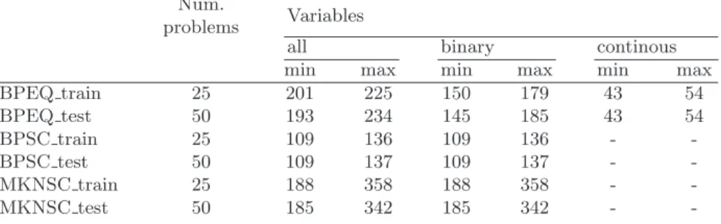
Random problems We randomly generate three sets of binary-integer or mixed binary-integer minimization problems that each contain two different types of constraints. The possible constraints are chosen among set cover (SC), multi-knapsack (MKN), bin packing (BP), and equality constraints (EQ). We generated problems that contain constraints of type BP-EQ, BP-SC and MKN-SC. The number of variables, the number of constraints, and the values of the elements in the matrices c, A and b are randomly generated. The number of vari-ables in these problems is of the order of a couple of hundreds, and the number of constraints is of the order of one hundred. As some of those problems are going to be used to generate the learning dataset, we split each family into a ‘train’ and a ‘test’ set. In the end, we have six datasets ‘BPEQ train’, ‘BPEQ test’, ‘BPSC train’, ‘BPSC test’, ‘MKNSC train’ and ‘MKNSC test’. The test sets contain 50 problems each, while the training sets each contain 25. Tables1and2
summarize statistics about the randomly generated problems. More specifically, those tables respectively contain the bounds on the number of variables and on the number of constraints of the problems contained in each randomly gener-ated set. Those datasets will be made available online or can be provided upon request.
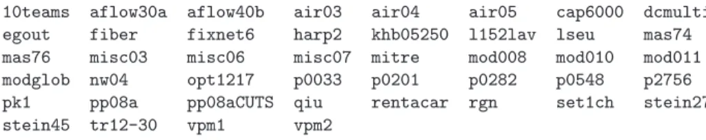
MIPLIB To compare the different branching strategies, we use the MIPLIB3 [9] and the MIPLIB2003 [3] problem sets. Indeed, in the integer programming com-munity, the MIPLIB problems are considered as the standard benchmark to compare different integer programming methods. From those two sets, we elim-inated the non-binary problems and the problems that were too big. Our final test set contains 44 problems. The complete list is given in Table3.
6.2 Experimental procedure
Our experimental procedure is composed of three steps: (1) we generate a dataset Dsb of pairs composed of features and strong branching scores, (2) we learn
from Dsba branching heuristic, and (3) we compare the learned branching
heuris-tic with other branching strategies on various problems.
Step 1: dataset generation In order to create a dataset of pairs (φi, si), we
apply the B&B with strong branching as branching heuristic on the problems contained in the sets ‘BPEQ train’, ‘BPSC train’ and ‘MKNSC train’, which we call training problems. At each node explored by B&B during the optimization of those problems, the strong branching score Bsb(i, c, A, b, x∗, l∗, u∗) = si is
computed for each fractional variable i ∈ F , together with the features φi asso-ciated with that variable at the current node. The computed strong branching score siis then normalized by the objective value at the current node, i.e. c⊤x∗,
Table 1. Random problem sets. ‘all’, ‘binary’ and ‘continuous’ respectively indicate the total number, and the number of binary and continuous variables in the problems.
Num.
problems Variables
all binary continous min max min max min max
BPEQ train 25 201 225 150 179 43 54 BPEQ test 50 193 234 145 185 43 54 BPSC train 25 109 136 109 136 - -BPSC test 50 109 137 109 137 - -MKNSC train 25 188 358 188 358 - -MKNSC test 50 185 342 185 342 -
-Table 2.Random problem sets. ‘all’, ‘EQ’, ‘BP’, ‘SC’ and ‘MKN’ respectively specify the total number, and the number of equality, bin packing, set covering and multi-knapsack constraints in the problem sets.
Constraints
all EQ BP SC MKN
min max min max min max min max min max BPEQ train 94 138 39 50 55 89 - - - -BPEQ test 94 135 39 50 53 89 - - - -BPSC train 80 110 - - 50 73 28 40 - -BPSC test 80 112 - - 50 75 27 39 - -MKNSC train 108 156 - - - - 61 77 42 84 MKNSC test 108 160 - - - - 58 77 43 89
such that the resulting normalized score represents a relative increase of the dual bound at the current node when variable i is selected for branching. This normal-ization is required to make sure that the score is independent of the scale of the problem. The pairs composed of features and normalized scores are then saved in the dataset Dsb, which is then used as input of the learning algorithm to
gen-erate the learned branching strategy Blearned(i, φi). Because strong branching is
a very slow heuristic, optimizing each training problem with strong branching until optimality is reached is intractable. We therefore limit the optimization time of each training problem to one hour. When it comes to generating the learning dataset, the size and the difficulty of the problems also matter. Indeed, the learned branching heuristic can only reflect the branching decisions found in the dataset. It is important that the dataset contains branching decisions from the beginning of the optimization as well as from the very bottom of the B&B tree. This consideration has to be taken into account when choosing the training problems. Indeed, as the learning dataset Dsbis generated with strong branching
(which is very slow) and because of the time limit, choosing a problem too hard or too big will produce a dataset in which branching decisions taken at the end of the optimization are missing. This is the reason why the problems that we consider in this work are rather small.
Table 3.List of problems from MIPLIB3 and MIPLIB2003
10teams aflow30a aflow40b air03 air04 air05 cap6000 dcmulti egout fiber fixnet6 harp2 khb05250 l152lav lseu mas74 mas76 misc03 misc06 misc07 mitre mod008 mod010 mod011 modglob nw04 opt1217 p0033 p0201 p0282 p0548 p2756 pk1 pp08a pp08aCUTS qiu rentacar rgn set1ch stein27 stein45 tr12-30 vpm1 vpm2
The dataset Dsb originally contains around 107 learning examples. Due to
memory limitations, we reduce this number to 105learning examples, randomly
selected from the original Dsb, which are then used to learn Blearned(i, φi).
Step 2: learning a branching heuristic We now apply a supervised machine learning algorithm to the dataset Dsb to learn a branching heuristic. In this
work, we use Extremely Randomized Trees [14], or ExtraTrees. Our choice is motivated by the simplicity and the computational efficiency of the ExtraTrees. Indeed, the performances of ExtraTrees are very robust against the choice of their parameters, and the default values provided in [14] work very well in practice. The ExtraTrees actually have three parameters: N , which is the number of trees in the method; k, which is the number of features evaluated at each node during the creation of the trees; and nmin, which is the number of training samples
contained in a node below which that node becomes a leaf. The number of trees is set to the default value of N = 100 in our experiments. The parameter k, which represents the number of features that are considered for the creation of the next node in the ExtraTrees, is also set to the default value of k = |φ|. The parameter nmincontrols the complexity of the trees. A small nmin yields bigger
trees, thus slowing down the prediction of a branching score from the features. Moreover, a small nmin might lead to overfitting the training set. On the other
hand, a larger nmin produces smaller trees that allow quicker predictions and
that reduce the amount of overfitting. We empirically set the value of nmin to
nmin= 20. The exact understanding of these parameters is beyond the scope of
this paper, and we refer the reader to [14] for a deeper explanation.
Step 3: comparing branching heuristics After having generated the dataset Dsb and applied the ExtraTrees, we compare our learned branching strategy
(learned) to five other branching heuristics namely random branching (ran-dom), most-infeasible branching (MIB), non-chimerical branching (NCB) [13], full strong branching (FSB) and reliability branching (RB) [2]. Random branch-ing is a branchbranch-ing strategy in which the branchbranch-ing variable is randomly chosen among the fractional variables. We use the perseverant version of non-chimerical branching [13], and the default parameter values λ = 4 and η = 8 for reliability branching [2]. The strong branching LP-relaxations are solved to optimality, and there is no limit on the number of candidate fractional variables at each node.
Two types of experiments are performed, where the optimization is early stopped based on a limit either on the number of explored nodes or on the time spent. The rationale behind those two experiments is to evaluate different aspects of the branching strategies. When the optimization is limited by the number of explored nodes, we can compare the branching strategies based on the closed gap3and on the time spent to actually explore that given number of nodes. This
sheds some light on how good the decisions taken by a branching strategy are compared to other branching strategies. This experiment also reveals the time needed to actually take a decision. In these conditions, FSB is usually the best in terms of closed gap and the worst in terms of time spent. On the other hand, the time limit is useful to assess different strategies in practical conditions where the number of nodes matters less than the time required to solve a problem. The closed gap is also used in that experiment to assess how far from the optimum the optimization is after a given amount of time. In this case, FSB is typically outperformed, in terms of closed gap, by other strategies.
The computations have been performed on a 16 cores computer composed of two Intel Xeon E5520 (2.27GHz, 8 cores) with 8MB cache and 32GB RAM running CPLEX 12.2. To assess only the performances of the different branching strategies, we disable heuristics, cuts and presolve in CPLEX. Furthermore, for each optimization, only one core is made available so that parallelism is disabled as well.
7
Results
We now present a selection of results comparing our approach to the other branching strategies (random, MIB, NCB, FSB, and RB). Tables 4, 5 and 6
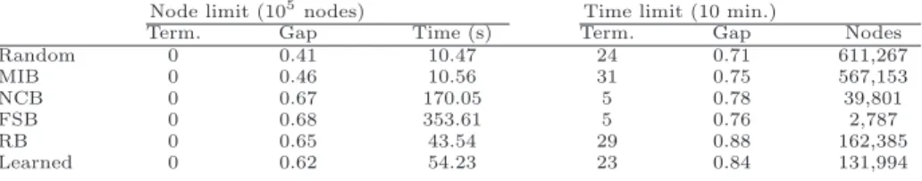
show these results. In these tables, ‘gap’ refers to the closed gap, and ‘term.’ in-dicates the number of problems that terminated within the given nodes or time limit. ‘Nodes’ and ‘time’ respectively represent the number of explored nodes and the time spent (in seconds) before the optimization either finds the opti-mal solution, or stops earlier because of one stopping criterion. Those values are measured separately for each problem and are averaged in the tables. We applied the six branching strategies on the random test problems (‘BPEQ test’, ‘BPSC test’ and ‘MKNSC test’) and on the selected MIPLIB problems.
7.1 Results for the randomly generated problems
Table4first shows the overall results achieved on the random test problem sets for both stopping criteria. Those results show that our approach succeeds in efficiently imitating FSB. Indeed, the experiments performed with a limit on the number of nodes show that the closed gap is only 9% smaller, while the
3
The closed gap (∈ [0; 1]) is the ratio of the difference between the current dual bound and the objective value of the initial LP-relaxation, to the difference between the optimal objective value and the objective value of the initial LP-relaxation. A value close to 1 indicates that the optimization is almost finished.
Table 4.Results for the problems of BPEQ test, BPSC test and MKNSC test.
Node limit (105
nodes) Time limit (10 min.)
Term. Gap Time (s) Term. Gap Nodes
Random 0 0.41 10.47 24 0.71 611,267 MIB 0 0.46 10.56 31 0.75 567,153 NCB 0 0.67 170.05 5 0.78 39,801 FSB 0 0.68 353.61 5 0.76 2,787 RB 0 0.65 43.54 29 0.88 162,385 Learned 0 0.62 54.23 23 0.84 131,994
Table 5.Results for the MIPLIB problems. Node limit = 105
nodes.
Solved by all methods Not solved by at least one method
Term. Nodes Time (s) Term. Gap Nodes Time (s)
Random 9 1,974 2.24 0 0.43 10,000 124.50 MIB 9 2,532 6.03 6 0.50 9,274 233.19 NCB 9 879 10.70 11 0.72 7,322 232.74 FSB 9 692 14.48 12 0.73 7,184 629.87 RB 9 1,123 15.78 10 0.64 7,806 219.39 Learned 9 1,194 2.73 10 0.62 8,073 162.87
Table 6.Results for the MIPLIB problems. Time limit = 10 min.
Solved by all methods Not solved by at least one method
Term. Nodes Time (s) Term. Gap Nodes Time (s)
Random 19 29,588 30.50 0 0.47 867,837 600.01 MIB 19 14,931 14.68 3 0.52 764,439 561.27 NCB 19 7,051 41.55 5 0.73 101,408 513.00 FSB 19 5,687 70.84 3 0.66 49,008 534.65 RB 19 6,895 27.38 7 0.69 257,375 515.40 Learned 19 14,008 34.12 5 0.63 130,081 512.72
time spent is reduced by 85% compared to FSB. The experiments with a time limit show that the reduced time required to take a decision allows the learned strategy to explore more nodes, and to thus further close the gap than FSB. While these results are encouraging, they are still slightly worse than the results obtained with RB, which is both closer to FSB and faster than our approach.
7.2 Results for the MIPLIB problems
Tables5and6show the results obtained respectively with a node limit and a time limit on the MIPLIB problems. In those experiments, we separated the prob-lems that were solved by all methods, from the probprob-lems that were not solved by at least one of the compared methods. Similarly to the results obtained on the random problem sets of Table4, the proposed branching strategy compares favorably with strong branching both on the node limit and time limit experi-ment. Nonetheless, the results obtained with the learned branching strategy are still a little below the results obtained with reliability branching.
8
Conclusion
In this paper, we proposed a new approach to design branching strategies for MILP problems that is based on supervised machine learning. The approach
consists in observing branching decisions taken by a supposedly good strategy, full strong branching (FSB) in our case, and to imitate those decisions. To this end, we develop a set of features that are used to characterize the current state of the problem in the B&B tree from the perspective of a particular variable. This set of features is then used as the input of the learned branching heuristic in order to predict the expected increase of the objective value that a branching on this variable would produce. The experiments show that our approach succeeds in approximating strong branching and in speeding up the decision process. However, the performances of our approach are still a little below state-of-the-art methods.
The underlying mechanism of our approach is not different from other pop-ular branching heuristics. Indeed, in both cases, features are computed from the current state of the problem, and then used to decide which variable to branch on. In our approach, however, we may include many types of features, including those used by the popular strategies. The approach is able to sort out which of those features are useful, and to automatically determine how to combine them to rank branching decisions. In that sense, we can see our method as a very general branching strategy that can imitate any other heuristic, as long as the appropriate features are provided. Our method can also discover novel heuristics by combining the features used by several popular methods with novel ones.
Further research orientations include the development of more relevant fea-tures that would allow the learned branching policy to get closer to strong branching. Another potential improvement direction could be to consider other more efficient and potentially more time-consuming branching strategies that could favorably replace strong branching as model for the machine learning al-gorithm.
Although our study in this paper is totally devoted to the imitation of FSB in the context of B&B on MILP problems, the same framework can be trans-posed to imitate any search heuristic deemed appropriate for solving any class of optimization problems.
References
1. Achterberg, T., Berthold, T.: Hybrid branching. In: Integration of AI and OR techniques in constraint programming for combinatorial optimization problems, pp. 309–311. Springer (2009)
2. Achterberg, T., Koch, T., Martin, A.: Branching rules revisited. Operations Re-search Letters 33(1), 42–54 (2005)
3. Achterberg, T., Koch, T., Martin, A.: Miplib 2003. Operations Research Letters 34(4), 361–372 (2006)
4. Achterberg, T., Wunderling, R.: Mixed integer programming: analyzing 12 years of progress. In: Facets of Combinatorial Optimization, pp. 449–481. Springer (2013) 5. Applegate, D., Bixby, R., Chv´atal, V., Cook, W.: Finding cuts in the tsp (a
pre-liminary report). Tech. Rep. 05, DIMACS (1995)
6. Benichou, M., Gauthier, J., Girodet, P., Hentges, G., Ribiere, G., Vincent, O.: Experiments in mixed-integer linear programming. Mathematical Programming 1(1), 76–94 (1971)
7. Berthold, T., Salvagnin, D.: Cloud branching. In: Integration of AI and OR Tech-niques in Constraint Programming for Combinatorial Optimization Problems, pp. 28–43. Springer (2013)
8. Bertsimas, D., Weismantel, R.: Optimization over integers, vol. 13. Dynamic Ideas Belmont (2005)
9. Bixby, R., Ceria, S., McZeal, C., Savelsbergh, M.: An updated mixed integer pro-gramming library: Miplib 3.0 (1996)
10. Dantzig, G.B.: Origins of the simplex method. Tech. rep., DTIC Document (1987) 11. Driebeek, N.J.: An algorithm for the solution of mixed integer programming
prob-lems. Management Science 12(7), 576–587 (1966)
12. Fischetti, M., Monaci, M.: Backdoor branching. In: Integer Programming and Com-binatoral Optimization, pp. 183–191. Springer (2011)
13. Fischetti, M., Monaci, M.: Branching on nonchimerical fractionalities. Operations Research Letters 40(3), 159–164 (2012)
14. Geurts, P., Ernst, D., Wehenkel, L.: Extremely randomized trees. Machine learning 63(1), 3–42 (2006)
15. Hutter, F., Hamadi, Y., Hoos, H.H., Leyton-Brown, K.: Performance prediction and automated tuning of randomized and parametric algorithms. In: Principles and Practice of Constraint Programming-CP 2006, pp. 213–228. Springer (2006) 16. Karangelos, E., Panciatici, P., Wehenkel, L.: Whither probabilistic security
man-agement for real-time operation of power systems? In: Bulk Power System Dynam-ics and Control-IX Optimization, Security and Control of the Emerging Power Grid (IREP), 2013 IREP Symposium. pp. 1–17. IEEE (2013)
17. Karzan, F.K., Nemhauser, G.L., Savelsbergh, M.W.: Information-based branching schemes for binary linear mixed integer problems. Mathematical Programming Computation 1(4), 249–293 (2009)
18. Land, A.H., Doig, A.G.: An automatic method of solving discrete programming problems. Econometrica: Journal of the Econometric Society pp. 497–520 (1960) 19. Li, C.M., Anbulagan, A.: Look-ahead versus look-back for satisfiability problems.
In: Smolka, G. (ed.) Principles and Practice of Constraint Programming-CP97, Lecture Notes in Computer Science, vol. 1330, pp. 341–355. Springer Berlin Hei-delberg (1997)
20. Marcos Alvarez, A., Maes, F., Wehenkel, L.: Supervised learning to tune simulated annealing for in silico protein structure prediction. In: ESANN 2012 proceedings, 20th European Symposium on Artificial Neural Networks, Computational Intelli-gence and Machine Learning. Ciaco (2012)
21. Moll, R., Barto, A.G., Perkins, T.J., Sutton, R.S.: Learning instance-independent value functions to enhance local search. In: Advances in Neural Information Pro-cessing Systems (1998)
22. Patel, J., Chinneck, J.W.: Active-constraint variable ordering for faster feasibility of mixed integer linear programs. Mathematical Programming 110(3), 445–474 (2007)
23. Schrijver, A.: On the history of combinatorial optimization (till 1960). Handbooks in Operations Research and Management Science: Discrete Optimization 12, 1 (2005)
24. Zhang, W., Dietterich, T.G.: A reinforcement learning approach to job-shop scheduling. In: IJCAI. vol. 95, pp. 1114–1120 (1995)