1/30 BEEF CATTLE METHANE EMISSION ESTIMATION USING THE EDDY COVARIANCE TECHNIQUE IN 1
COMBINATION WITH GEOLOCATION 2
P. Dumortier1, L. Gourlez de la Motte1, A.L.H. Andriamandroso1, M. Aubinet1, Y. Beckers1, J. Bindelle1,
3
N. De Cock1, F. Lebeau1 and B. Heinesch1
4
1University of Liege, Gembloux Agro Bio-Tech, TERRA Teaching and Research Center, Belgium
5
6
Abstract
7Methane emissions of a grazing herd of Belgian Blue cattle were estimated per individual on the field 8
by combining eddy covariance measurements with geolocation of the cattle and a footprint model. 9
This method allows the measurement of outdoor non-invasive methane emissions but is complex and 10
subject to methodological issues. Estimated emissions were 220 ±35 g CH4 LU−1 day−1 (grams of
11
methane per livestock unit per day), where the uncertainty corresponds to the random error and does 12
not include any possible systematic error. Cattle behavior was also monitored and presented a clear 13
daily pattern of activity with more intense grazing after sunrise and before sunset. However, no 14
significant methane emission pattern could be associated with it, the diurnal emission variation being 15
lower than the measurement precision. 16
Key-words: eddy covariance, methane, cattle, footprint, geolocation 17
Graphical Abstract
182/30 19
1 Introduction
20Ruminants are able to digest cellulose which makes them incredibly apt to transform raw forage, like 21
grass, into high quality products. This digestive characteristic is due to an association with a very 22
specific microbial flora present in the rumen or hindgut which allows the transformation of complex 23
plant material into digestible fatty acids (acetate, lactate, propionate or butyrate). However, this 24
transformation is accompanied by the co-production of methane, a potent greenhouse gas, which is 25
mostly released through eructation (Broucek, 2014). 26
The current standard measurement method for cattle methane emissions is the metabolic chamber. 27
This method calculates a mass balance between methane entering and leaving a sealed ventilated 28
chamber containing an animal. Tracer methods are the major alternative for grazing ruminants; they 29
involve the use of an external (e.g., SF6 released by an ingested canister) or internal (e.g., metabolic
30
CO2 emissions) tracer released at a known rate from the animal’s rumen. Measuring tracer and
31
methane concentration ratios in excreted gases allows the computation of methane fluxes. Both 32
techniques are accurate with a precision commonly higher than 90%, but require lots of animal 33
Each cow is equipped with a GPS unit and an accelerometer Eddy covariance mast Footprint function 220 ±35 g CH4 LU−1day−1 Estimation of cattle methane emissions
3/30 handling (Storm et al., 2012), are rather invasive and could impact the natural grazing behavior of 34
cattle. Emerging methods rely on the use of proxies; they are based on the relationship between 35
methane emissions and the composition of matrices that are easy to sample such as feces or milk 36
(Dehareng et al., 2012; Vanlierde et al., 2018). This method is valid as long as the composition of the 37
proxies and the characteristics of the sampled animals (i.e., breed, intake level, physiological status, 38
etc.) remain within the range of variability of the database that was used to develop the relationship. 39
In addition to these animal-centered approaches, measurement methods have been developed that 40
work at the scale of the environment in which the animals evolve. Some of these techniques simply 41
reproduce lower scale methods (i.e., by considering the barn or the feeding trough as a chamber or by 42
adding a tracer gas in a ventilated barn at a known rate and measuring the methane/tracer ratio) while 43
others involve micro-meteorological methods (Johnson and Johnson, 1995; Storm et al., 2012). The 44
latter are promising because they allow measurements to be recorded of the emission rate of the 45
whole herd, on the field, with a half-hour time resolution, little animal handling and without disturbing 46
the cow’s natural behavior. Among micrometeorological methods, eddy-covariance (EC) is well suited 47
for measurements in a pasture with low cattle density over large areas, and has become more 48
affordable with the release of fast and precise optical methane analyzers. Nevertheless, applying this 49
measurement method to grazed pastures is challenging due to a combination of source complexity 50
(i.e., spatial and temporal variation in animal locations and emission intensities) and limitations in 51
methodology specific to EC (Dumortier et al., 2017; Wohlfahrt et al., 2012). 52
Cattle emissions are not constant over time. Most of the CH4 produced escapes through the mouth,
53
with 83% of emissions associated with eructation and 15% associated with respiration (Hammond et 54
al., 2016). Cattle eruct 15 to 28 times each hour (every 130 to 230 s) according to the composition of 55
their diet, feed intake levels and physiology (Blaise et al., 2018). Moreover, methane emissions vary 56
throughout the day, peaking approximately 2 hours after feeding followed by a decrease until the next 57
feeding event (Blaise et al., 2018). Cattle methane emissions thus present a 24-hour emission pattern 58
which can be related to their feeding behavior (Hammond et al., 2016; Hegarty, 2013). 59
4/30 When using EC, the measured covariance corresponds to the vertical flux at one specific point that is 60
representative of exchanges within the footprint, the area “sensed” by the flux measurement device. 61
This footprint can be modeled through a set of functions that weight the respective contribution of 62
each element of the surface to the measured vertical flux (Rannik et al., 2012), known as a footprint 63
model. However, animals act as moving CH4 sources which may wander in or out of the footprint.
64
Therefore, fluxes measured through eddy covariance must be combined with a footprint model as well 65
as information about the cattle’s location on the pasture in order to estimate the animals’ contribution 66
to the measured flux. The ability of this approach to provide reliable emission estimates was previously 67
tested using artificial sources (Dumortier et al., 2019). Previous investigations by Heidbach et al. (2017) 68
showed that the FFP (Flux Footprint Prediction) model presented by Kljun et al. (2015) was the most 69
efficient of the four tested models as long as the artificial source was located further from the mast 70
carrying the sensors than the footprint peak (maximum of the footprint function). One of the main 71
drawbacks of this model is that sources are assumed to be at ground level, while cattle emissions are 72
emitted at muzzle height (i.e., up to 1 m height). To tackle this issue, Coates et al. (2017) simulated 73
free-range cattle with artificial methane sources scattered on a field at a height of 0.8 m. They were 74
able to estimate artificial source emissions with an error of 10% regardless of the distance between 75
the source and the mast by using a Lagrangian stochastic model which could consider source heights. 76
Because stochastic approaches require high computational power, Dumortier et al. (2019) tried to 77
assess to what extent ready-to-use footprint models, that do not consider source height, could be 78
stretched beyond the conditions for which they were designed in order to estimate methane emissions 79
from elevated artificial sources. They concluded that emissions could be correctly estimated (error of 80
less than 15%) using the analytical Kormann & Meixner (2001) footprint model when the artificial 81
source was located further from the mast than the footprint peak. 82
These results strengthen the idea that EC can be used to estimate point source emissions of methane 83
from cattle in field conditions. Felber et al. (2015) were the first to put this idea into practice. They 84
calculated an emission per dairy cow by combining EC with cow geolocation data and the Kormann & 85
5/30 Meixner (2001) footprint model. The experiment was run on a 3.6 ha pasture divided into 6 paddocks 86
which were either very close to or distant from the mast. Every few days animals were transferred 87
from one paddock to another (rotational grazing). This resulted in high stocking densities at the pasture 88
level (5.5 LU ha−1; LU, livestock unit) but very high stocking densities in the occupied paddock (up to
89
33 LU ha−1). For paddocks close to the mast (less than 60 m), measured methane emission levels
90
compared reasonably well (difference of less than 5%) with those obtained from metabolic chambers 91
hosting dairy cows with similar milk production levels and body weights. However, for paddocks more 92
distant from the mast, measured emissions per animal were lower and compared poorly to metabolic 93
chambers, suggesting an imprecision of the footprint model. Other authors have successfully used a 94
similar approach in different contexts (Prajapati and Santos, 2017), researching different gases 95
(Gourlez de la Motte et al., 2019) or using different footprint tools (Coates et al., 2018). 96
In this work, free ranging cattle methane emissions on the pasture are estimated by combining eddy 97
covariance with geolocation. This approach provides a variety of situations with the herd at rest, 98
gathered at various distances from the mast, and cows more dispersed on the pasture during grazing. 99
Moreover, we are able to rely on a methane emission estimation method previously validated on the 100
same site with an artificial tracer (Dumortier et al., (2019). Our main objectives are: 101
To adapt an existing method combining the EC technique and a footprint model (Dumortier et 102
al., 2019) with cattle geolocation data in order to estimate mean enteric emissions per 103
livestock unit (LU). The validity of this approach is estimated by the internal consistency of the 104
results (stability of emissions, uncertainties and impact of meteorological conditions). 105
To estimate methane emissions of Belgian Blue cattle on a typical Belgian commercial farm 106
and to compare these with existing estimates (including IPCC default values). 107
To investigate the relation between methane emissions and cattle behavior. 108
6/30
2 Materials and Methods
109
2.1 Experimental site
110The ICOS-candidate Dorinne Ecosystem Station (BE-Dor) is a 4.2 ha pasture located in Dorinne, Belgium 111
(location: 50˚18’42.84”N; 4˚58’4.8”E; 248 m above sea level). The site is the location of previous 112
investigations and is fully described in Dumortier et al. (2017) and in Gourlez de la Motte et al. (2019). 113
The pasture is situated on a loamy plateau with a calcareous and/or clay substrate. Its species 114
composition is: 66% grasses, 16% legumes and 18% other species. The dominant species are perennial 115
ryegrass (Lolium perenne L.) and white clover (Trifolium repens L.). The pasture is used for cow-calf 116
grazing operations with Belgian Blue cattle with a mean annual stocking density in the pasture (SDp) of
117
2.0 LU ha−1 (livestock unit per ha). An eddy-covariance measuring mast is located in the center of the
118
pasture (Figure 1). Wind speed and direction are measured on this mast using a sonic anemometer 119
(CSAT3, Campbell Scientific Ltd, UT, USA) at a height of 2.6 m. Air sampled near the anemometer 120
(0.216 m N, 0.125 m E and 0.23 cm below) is carried through a 2 µm filter (SS-4FW4-2, Swagelok 121
Company, OH, USA) and a heated PTFE tube (inner diameter 3.18 mm, length 6.85 m, flow rate 9 122
10−5 m3 s−1) to the fast methane analyzer (G2311-f, Picarro, Inc, CA, USA).
7/30 124
Figure 1. Satellite view from the Dorinne Ecosystem Station. The pasture is highlighted in white, the red cross indicates the 125
mast and the black ellipse indicates the location of the barn. 126
Four measurement campaigns were organized involving 8 to 19 cows weighing between 700 and 127
850 kg, up to one breeding bull (±1300 kg) and up to 19 calves (Table 1). During each of these 128
campaigns, cattle positions and behavior were monitored as described in §2.2, fluxes were measured 129
as described in §2.3, and cattle emissions were computed as described in §2.4. 130
Table 1. Description of the four measurement campaigns. 131
Campaign Start and end date Number of cows /calves Stocking density [LU ha−1] Main wind direction Spring 2014 27 May 2014 – 25 Jun 2014 17-19 /17-19 6 N-E N
8/30 Spring 2015 14 Apr 2015 – 7 May 2015 12 /0 2.8 S-W Summer 2015 14 Aug 2015 – 2 Sept 2015 12 /10 3.8 S-W Autumn 2015 19 Oct 2015 – 2 Nov 2015 8 /0 1.9 S-E
2.2 Position and behavior monitoring
132During the four measurement campaigns, the position and behavior of each adult cow were monitored 133
using a homemade tracking device consisting of a GPS unit and an accelerometer which was located 134
on the top of the cow’s neck (Figure 2). Data were collected by a GPS antenna module (Fastrax UP 501, 135
Fastrax Ltd., Finland) and a low power 3 axis accelerometer (ADXL335, Analog Devices Inc., MA, USA) 136
and were stored on a micro SD card. Power was supplied by four batteries (3.8 V, 4 × 2000 mAH). The 137
tracker could work for approximately 30 days on a single charge, avoiding too frequent handling of 138
cows for battery replacement. In order to reach this autonomy, the data collection had to be 139
discontinuous. Every 5 minutes, the tracker would wake up, wait for the acquisition of at least 3 140
satellite signals (which typically took about 30 s), record the position and acceleration components 141
(used to detect behavior) in 3 dimensions at 20 Hz for 20 s, and then return to sleep mode. Neither the 142
calves nor the bull were equipped with tracking devices. The GPS module precision was assessed by 143
leaving the device motionless at a known position in the pasture for 41 days. During this period, 50% 144
of the points were found within 3 m of the true location, 76% within 5 m and 95% within 11 m. 145
For animals which were not correctly geolocated (GPS malfunctions, representing 3.7 to 18.8% of the 146
dataset from one campaign to another, or calves), their contribution to the footprint had to be 147
estimated, resulting in an additional correction. Cattle footprint contributions were corrected by a 148
geolocation correction factor (GCF) using Equation 1, with a cow corresponding to 1 LU and a calf (4 to 149
10 months) to 0.4 LU. Data were excluded from the dataset when the GCF was larger than 1.5 (up to 150
9/30 56% of the dataset for the Spring 2014 campaign). The calves’ conversion factor of 0.4 is based on the 151
Walloon region criteria for the Common Agriculture Policy (“Arrêté ministériel exécutant l’arrêté du 152
Gouvernement wallon du 3 septembre 2015 relatif aux aides agro-environnementales et climatiques”) 153
and is in agreement with the estimated emission levels of calves which should be between 30 and 40% 154
of an adult cow (Basarab et al., 2012; Dämmgen et al., 2013; Lockyer, 1997). 155
𝐺𝐶𝐹 =∑ 𝐿𝑈 𝑜𝑛 𝑡ℎ𝑒 𝑝𝑎𝑠𝑡𝑢𝑟𝑒∑ 𝐷𝑒𝑡𝑒𝑐𝑡𝑒𝑑 𝐿𝑈 (1)
156
157
Figure 2. Position and activity tracking device represented with the three axis system of the accelerometer. 158
Cattle behavior was sorted into three categories (grazing, ruminating and other) on the basis of the 159
acceleration mean value and standard deviation along the x-axis as represented in Figure 2. The use of 160
the x-axis was selected because it was discriminating and had a physical interpretation. The measured 161
acceleration can be divided into two terms: a low frequency component which corresponds to gravity 162
projection along each axis and allows identification of the cattle’s neck position, and a high frequency 163
component due to the cattle’s movements (Andriamandroso et al., 2016). During grazing, the cow’s 164
neck is oriented downward (positive values of ax,the mean x acceleration component) and is moving
165
abruptly for each bite (high ax, the standard deviation of this value), while during rumination the cow’s
166
neck is horizontal or raised slightly upwards (ax, values close to 0 ms‒² or slightly negative) with small
167
movements related to mastication (low ax). Other behaviors are characterized by a large array of ax
168
and ax values, which sometimes overlap with rumination or grazing characteristic values
169
(Andriamandroso et al., 2017). Attributing a behavior using universal absolute thresholds of ax and ax
170
x
z
y
10/30 was not possible due to the specific positioning of the device on each cow. However, as cattle spend 171
approximately 60% of their time grazing and 15% ruminating (Braghieri et al., 2011), these behaviors 172
were detected by an algorithm which was looking for combinations of ax and ax occurring more
173
frequently. For each cow-collar combination, a 2D histogram was created with 20 categories of ax and
174
20 categories of ax. For each of these 400 categories (20 × 20), the ones with the highest occurrence
175
(threshold set at 3 times the average occurrence) were considered as rumination or grazing according 176
to ax and ax (Figure 3).
177
178
Figure 3. Scatterplot of acceleration characteristics along the x-axis for a single cow and during a single measurement 179
campaign. The horizontal axis corresponds to the mean acceleration and the vertical axis corresponds to the standard 180
deviation. Each point represents a 20 s sample and is automatically associated with a behavior by an algorithm. 181
The precision of the behavior detection method was assessed by comparison to the behavior of cows 182
which were visually observed for two hours, resulting in the acquisition of 115 5-minute measures. 183
Those results are presented in Table 2. Detected behaviors agreed with observations in 85, 80 and 23% 184
of the time for grazing, rumination and other behaviors respectively, while observations agreed with 185
11/30 detections 96, 45 and 38% of the time for grazing, rumination and other behaviors respectively. This 186
means that the grazing behavior was well characterized, while rumination and other behaviors where 187
poorly distinguished. 188
Table 2. Confusion matrix of the behavior detection algorithm. Each row of the matrix represents the instances in a 189
predicted class while each column represents the instances in an observed class. 190
Observation
Prediction
Grazing Rumination Other Total
Observation corresponding to prediction Grazing 48 0 2 50 96% Rumination 0 20 24 44 45% Other 8 5 8 21 38% Total 56 25 34 115 Prediction corresponding to observation 86% 80% 24%
2.3 Flux measurement and processing
191Turbulent methane fluxes were calculated using EddyPro® version 6.2.2 open source software (Li-Cor 192
Inc., NE, USA). The computation was the same as the method used by Dumortier et al. (2019) with the 193
exception of the averaging period (30 minutes instead of 15 minutes) due to the presence of outliers 194
that could not be filtered for the 15-minute averaging interval. The main differences from the default 195
calculation method were the use of a running mean with a 120 s time constant, and the absence of 196
stationarity filtering because animals could cause sudden fluctuations in the methane dry mixing ratio. 197
12/30 Time lags between measured vertical velocity and methane dry mixing ratio were calculated using a 198
covariance maximization method with a default value of 2.3 s and a window size of 1 s (79% of the 199
records were found within this time window for methane). A correction for high-frequency losses was 200
applied using an in situ spectral correction method (Fratini et al., 2012). Data were also filtered on the 201
basis of friction velocity, using a u* threshold of 0.13 m s−1 (Dumortier et al., 2017; Gourlez de la Motte
202
et al., 2016). Among the statistical tests for raw data screening proposed by Vickers and Mahrt (1997), 203
some choices were made. The spike filtering, drop-out, absolute limit and discontinuities tests were 204
applied using the default settings proposed in EddyPro®. These tests removed less than 3% of the 205
dataset. Amplitude resolution, skewness and kurtosis tests were disabled as in a previous artificial 206
source campaign (Dumortier et al., 2019); they induced a removal of almost all periods involving the 207
artificial source in the footprint, although these signal characteristics were obviously generated by a 208
real phenomenon. 209
An additional filter was added to remove data associated with poorly defined footprint functions 210
(z/L>0.05). Moreover, as cattle muzzles are not found solely at ground level but at a height ranging 211
from ground level to approximately 0.8 m high, a minimum distance between the source and the mast 212
was defined. The impact of the source height had been tested using FIDES (Loubet et al., 2010), a 213
pseudo Gaussian footprint model which includes the height of the source as an input variable. The 214
conclusion was that for a source located further than 12 m from the mast for unstable conditions and 215
16 m from the mast for neutral conditions, the source height impact on the footprint function was 216
below 15% if the source is found below 0.8 m. These distances were therefore selected for data 217
filtering. 218
The footprint function extended well beyond the pasture borders (Figure 4) which means that events 219
occurring outside of the pasture could be unintentionally detected. This was the case during the Spring 220
2015 campaign which started early in the season (14 April), resulting in contaminated fluxes originating 221
from the barn (Figure 1) which was a strong methane source when cattle were still housed indoors, 222
13/30 and from a manure heap located 500 m south-west from the mast. For this campaign, contaminated 223
wind directions (5 to 50 and 200 to 230° N, clockwise) were thus removed from the dataset. Other 224
campaigns were not affected by these issues as, for later dates, no (or only a few) cows were present 225
in the barn and the manure had been used for crop fertilization. 226
227
Figure 4. Mean cumulative footprint during the whole measurement period using the Kormann & Meixner footprint 228
model. The isopleths represent the area responsible for x% of the measured flux (proportion of the footprint found 229
inside a specific area). The bold line corresponds to the pasture limits. 230
Applied filters and associated data loss are described in Table 3. According to this table, the proportion 231
of high quality flux data (meaning data without instrument malfunctions and with u* above 0.13) was
232
between 40 and 67% from one period to another. Moreover, 60 to 80% of the remaining dataset was 233
eliminated due to poorly defined cattle contribution to the footprint (which corresponds to a z/L ratio 234
above 0.05), unavailable cattle positions (GCF above the threshold), presence of cattle too close to the 235
mast (12 to 16 m according to meteorological conditions) or wind coming from a strong and undesired 236
14/30 methane source (barn or manure heap) for the Spring 2015 campaign. The remaining high quality 237
dataset was used for this study. No filter was associated to a minimum cattle contribution to the 238
footprint. 239
Table 3. Number (and percentage) of half-hours remaining after the application of each filtering step for each 240
measurement campaign. 241
Spring 2014 Spring 2015 Summer 2015 Autumn 2015
Measurement period 1385 1097 913 669
High quality flux data 859 (62%) 730 (67%) 415 (45%) 267 (40%) + Well defined cattle
contribution to the footprint
299 (22%) 136 (12%) 156 (17%) 171 (26%)
242
2.3.1 Enteric emission estimation
243
Methane emissions per LU (fCH4) were estimated according to the method described by Dumortier et
244
al. (2019), which is equivalent to the method proposed by Felber et al. (2015). fCH4 were computed by
245
combining turbulent flux measurements with cattle positions through the use of a footprint function 246
using Equation 2, where 𝐹𝐶𝐻4 is the measured methane flux (nmole m−2 s−1), i corresponds to the cow
247
identification number and 𝜙𝑖 the value of the footprint function at the i cow location (m−2). As cattle
248
locations were recorded every 5 minutes, the one sixth ratio allows the calculation of an average 𝜙𝑖
249
for each 30-minute interval as each animal occupied 6 locations during an averaging interval. 250
𝑓𝐶𝐻4=
𝐹𝐶𝐻4
𝐺𝐶𝐹×16∑ 𝜙𝑖 𝑖 (2)
251
where 𝐺𝐶𝐹 ×16∑ 𝜙𝑖 𝑖 corresponds to the stocking density in the footprint (SDf). The footprint function
252
(𝜙) was calculated according to the footprint model described by Kormann & Meixner (2001)(KM) on 253
15/30 a 30-minute averaging period. However, fCH4 values estimated through this method were subject to
254
high variations, especially for low SDf. A method more robust than a division was therefore considered.
255
Equation 2 implies a direct relationship between measured methane fluxes and cattle density in the 256
footprint. In other words, fCH4 can be calculated as the slope of the linear regression associated with
257
the relation between SDf and the measured methane flux. Different regression methods can be used
258
to infer the slope of the linear regression. The most common one, the Linear Least Square regression 259
(LLS) minimizes residues associated with the vertical axis and supposes no uncertainty associated with 260
the horizontal axis. However, when uncertainties are associated with both axes, as was the case here, 261
functional relations must be used (Webster, 1997). The Reduced Major Axis method (RMA, Matlab 262
code provided by Trujillo-Ortiz & Hernandez-Walls (2020)) minimizes residues along the normalized 263
horizontal and vertical axis, this method is therefore able to deal with uncertainties on both axes. 264
Another way to estimate the slope of the regression is the Median-Median Regression (MMR) which 265
is obtained by dividing the dataset into two groups (based on the median value of the x axis). For each 266
group the central point is calculated as the median value along horizontal and vertical axes. The 267
regression line then corresponds to the line passing through the center of each group. The main 268
advantage of the MMR method is that it doesn’t involve a hypothesis about the distribution shape or 269
the uncertainty associated with each axis. We applied these last two methods (RMA and MMR) to our 270
dataset, resulting in two fCH4 estimates. Both methods were far more robust than a simple division. For
271
both options, the confidence interval of the slope was estimated through a bootstrapping method. 272
This resampling method is adapted to almost any distribution and allows numerical estimation of the 273
uncertainty of the parent population and not only of the sample. The 95% confidence interval was 274
computed as the 2.5 and 97.5 percentile of the slope distribution after 5000 draws, and the 95% 275
uncertainty range corresponded to the half of this confidence interval. 276
16/30
3 Results
277
3.1 Cattle behavior and distribution
278For each campaign, cattle were found to be well spread over the whole pasture when grazing, while 279
they gathered near the water troughs and the trees bordering the pasture when ruminating or idling 280
(Figure 5). We also observed that grazing behaviors followed a diurnal pattern; animals grazed mainly 281
during the day with peak activities just after sunrise and before sunset (Figure 6). This behavior was 282
confirmed by GPS trackers which revealed a strong correlation between cattle movement and grazing 283
behavior. Cows were covering larger distances during the 5-minute interval between two consecutive 284
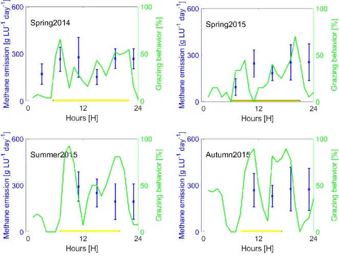
measurements when they were grazing (Figure 6). These results confirm the validity of the animal 285
behavior detection method presented in §2.2. 286
One might wonder if cattle geolocation was really necessary in order to estimate fCH4. Without
287
information about cattle’s location, fCH4 could be estimated for each campaign considering a
288
homogeneous cattle disposition in the pasture as done by Dumortier et al. (2017). However, as showed 289
in Figure 5, cattle disposition on the pasture is generally heterogeneous. The only notable exception is 290
during grazing events which are observed at sunrise and sunset. These periods could thus be used to 291
estimate cattle emissions without requiring any knowledge about cattle location. 292
17/30 293
Figure 5. Density maps of cows’ positions when grazing (A) or expressing other behaviors (B) for all four campaigns 294
combined. The black line represents the limits of the pasture. The occupancy is calculated as the percentage of the time 295
18/30 spent by cattle in each square meter. A homogeneous cattle distribution would result in a 0.06% occupancy over the whole 296
pasture. 297
298
Figure 6. Average percentage of the herd grazing (green) and distance covered between each measurement (black; each 5 299
minutes) according to the time of day for all four campaigns combined. 300
3.2 Enteric methane emissions
301Enteric methane emissions were estimated by the slope of the linear regression associated with the 302
relation between SDf and measured methane fluxes. In Figure 7, the two selected regression lines are
303
drawn for the Spring 2014 campaign, along with the LLS regression line for comparison purposes. The 304
slope of these regression lines were used to estimate fCH4. For each campaign, fCH4 values are
305
represented in Table 4. As slopes estimated using the RMA method were more stable and associated 306
with smaller confidence intervals, this method was selected for the rest of the paper. Over the course 307
of all four campaigns, fCH4 obtained using RMA was found to be between 184 and 255 (95% confidence
308
intervals) which corresponds to 220 ±35 g CH4 LU−1 day−1. This indicates an estimated random error of
19/30 16%. No significant differences in methane emission levels were observed between campaigns 310
(overlapping confidence intervals). 311
312
313
Figure 7. Relation between measured methane flux and stocking density in the footprint (SDf) calculated according to the 314
Kormann & Meixner footprint model for the Spring 2014 campaign with each point corresponding to a 30-minute 315
measurement interval. The different regression lines correspond to the reduced major axis method (RMA), the linear least 316
square (LLS) and the median-median regression method (MMR) (see §2.3.1 for more details about each method). 317
Table 4. Estimated cattle emissions per livestock unit (fCH4) for each campaign using two different methods: reduced 318
major axis regression (RMA) and median-median regression (MMR). All estimations are presented through a 95% 319
confidence interval and a 95% uncertainty range. 320 Campaign RMA [g CH4 LU−1 day−1] MMR [g CH4 LU−1 day−1] Spring 2014 188 – 268 168 – 266
20/30 228 ± 40 217 ± 49 Spring 2015 158 – 237 197.5 ± 39.5 93 – 415 254 ± 161 Summer 2015 137 – 321 229 ± 92 125 – 426 275.5 ± 150.5 Autumn 2015 172 – 270 221 ± 49 166 – 409 287.5 ± 121.5 All seasons 185 – 255 220 ± 35 183 – 254 218.5 ± 35.5
The uncertainty associated to a measurement method is critical when assessing its ability to quantify 321
emissions and, more importantly, to identify the impact of any mitigation of this emission. The error 322
associated with fCH4 estimates can be divided into two categories: the precision, which can be dealt
323
with by increasing the size of the dataset, and the accuracy, which is associated with the method and 324
was previously analyzed at the same site by Dumortier et al. (2019). In order to investigate the impact 325
of the size of the dataset on the random error associated with cattle CH4 emissions estimates, a
326
bootstrapping method was used (a random part of the dataset was sub-sampled) (Figure 8). Using this 327
method, we observed that at least 480 valid half-hours are needed in order to obtain a 95% uncertainty 328
range below 20%, while only 190 measures are needed in order to obtain an uncertainty range below 329
30%. 330
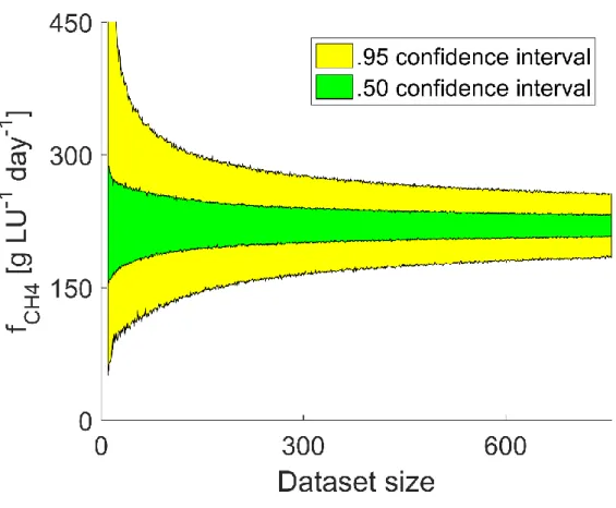
21/30 331
Figure 8. Impact of the size of the dataset on methane emissions per livestock unit (fCH4) confidence intervals estimated 332
using a bootstrapping method. For each possible size of the dataset, 5000 sub-samples were analyzed in order to compute 333
associated fCH4 estimates. For x% of those runs, estimated fCH4 values were found within the .x confidence interval, x 334
corresponding to 95 (yellow) or 50 (green). 335
Quantifying the relation between the uncertainty range and the size of the dataset allows an 336
estimation to be made of the amount of data required when designing an experiment. If one wishes 337
to be able to distinguish a significant impact of a specific mitigation action, the amount of data required 338
to observe differences above a certain threshold can be estimated. However, this uncertainty 339
estimation method is numeric and only based on our dataset. Other sites may provide different 340
relations between methane fluxes and stocking densities in the footprint, leading to different curves. 341
This result is thus difficult to extrapolate to other datasets. 342
3.3 Relations between cattle behavior and emissions
343During each campaign cattle mainly grazed after sunrise and before sunset, with intermediate grazing 344
events during the day when the photoperiod was long or during the night on shorter days (Figure 9). 345
However, significant fCH4 variations throughout the day were only observed for the Spring 2014 and
22/30 Spring 2015 campaigns where emissions were significantly lower for one 4-hour period (2 to 6 pm and 347
6 to 10 am respectively). Due to this very weak fCH4 diurnal variation, no detection of any significant
348
impact of cattle behaviors on methane emissions was possible. 349
350
Figure 9. Methane emission per livestock unit (fCH4) evolution throughout the day for each measurement campaign 351
computed with the reduced major axis (RMA) regression method and the Kormann & Meixner footprint model. The 352
whiskers indicate the 95% uncertainty range of fCH4 for each 4-hour period (bootstrapping). The green line indicates the 353
percentage of animal grazing and the yellow strip indicates the photoperiod for this specific time of year. Whiskers are 354
only represented when more than 10 points were available for a given interval. 355
An impact of the time since grazing peak was assessed when all campaigns were grouped together 356
(Figure 10). However, no significant impact of this time on cattle methane emissions was observed. 357
23/30 358
Figure 10. Methane emissions per livestock unit (fCH4) according to time since grazing peak for all campaigns together. 359
Times since grazing peak were organized into 3 categories containing the same number of samples and plotted as the 360
category mean. The error bars correspond to the 95% confidence intervals of fCH4 (bootstrapping method). The dotted line 361
indicates the fCH4 estimated using all data. All values have been computed with the RMA regression method and the KM 362
footprint model. 363
3.4 Cattle methane emissions bias analysis
364Atmospheric conditions or cattle movements on the pasture should not have any impact on estimated 365
fCH4. Nevertheless, in order to detect possible biases, such relations were examined. We observed no
366
significant impact (largely overlapping confidence intervals) of the distance between the closest cow 367
and the mast, atmospheric stability, u*, average distance covered by animals and wind direction on
368
estimated fCH4. For each variable and when using the complete dataset (all four campaigns grouped
369
together), significant relations were assessed after dividing the dataset into 3 equal size categories of 370
the selected variable. The absence of an impact of u* (even for values below 0.13 m s−1), of the distance
371
between cattle and the mast (even when below 12 m) or atmospheric conditions (even for z/L values 372
24/30 above 0.05) does not indicate the absence of bias from any of the previously listed variables on fCH4
373
but rather that the bias is lower than the uncertainty range associated with the measurements (relative 374
95% uncertainty ranges around 27% when the dataset was subdivided into 3 categories). 375
4 Discussion
3764.1 Validity of the method
377The first objective was to provide estimates of the mean enteric CH4 emissions per livestock unit by
378
combining the EC technique with a footprint model and cattle geolocation data. The combination of 379
EC with geolocation allows stable and realistic estimations of cattle methane emissions to be made 380
with measurement campaigns as short as one month (197 to 229 g CH4 LU−1 day−1). Obtained methane
381
emissions were realistic and the regression slope 95% uncertainty range was estimated between 18 382
and 40% for each campaign, despite the heterogeneous distribution of cattle on the pasture. As already 383
highlighted by Gourlez de la Motte et al. (2019), cattle were not homogeneously dispersed on the 384
pasture at all times (Figure 5). Therefore the use of GPS trackers was a great improvement compared 385
with the homogeneous cattle distribution hypothesis. As a result, the assumption used in Dumortier 386
et al. (2017) that cattle are spread homogeneously over the pasture is only valid when cattle are 387
grazing. This might explain why the homogeneous cattle distribution hypothesis can lead to good 388
results if cattle are confined in a delimited area, upwind from the mast, whose average footprint 389
contribution is known (Dengel et al., 2011; Dumortier et al., 2017; Felber et al., 2015). 390
4.2 Belgian Blue CH
4emissions
391
The second objective was to estimate methane emissions for the Belgian Blue breed on a typical 392
Belgian commercial farm and to compare these values with existing estimates. When averaging all four 393
campaigns, estimated emissions were 220 ±35 g CH4 LU−1 day−1 or 80 ±13 kg CH4 LU−1 yr−1. These
394
values are very close to tier 2 IPCC emission estimates (IPCC, 2006) of 205 ±41 g CH4 LU−1 day−1,
395
considering a measured average dry matter ingestion of 9.5 kg per day (Gourlez de la Motte et al., 396
2016), a default raw energy content of 18.45 MJ kg−1, a default methane conversion factor of 6.5% and
25/30 a default uncertainty range of 20%. The values are also very close to a previous measurement of 398
223 ±16 g CH4 LU−1 day−1 obtained by De Mulder et al. (2018) on the same breed using metabolic
399
chambers (indoor-housed Belgian Blue heifers). On the whole, the random error associated with fCH4
400
estimates was 16% (35 g CH4 LU−1 day−1).
401
The random error associated with emission estimates does not give any information about the 402
measurement accuracy. Our best estimate of this accuracy is obtained from the artificial source 403
experiment run on the same site (Dumortier et al., 2019). A recovery rate between 90% and 113% was 404
obtained, according to the distance between the source and the mast. For comparison, a 13% 405
systematic error on fCH4 estimates would translate to approximately 30 g CH4 LU−1 day−1.
406
4.3 Impact of cattle behavior on CH
4emissions
407
The third objective was to investigate the relation between methane emissions and cattle behavior. 408
The 95% confidence interval of fCH4 estimates depends on the number of observations. Therefore,
409
when the dataset was subdivided, uncertainty on binned estimations increased, making it difficult to 410
demonstrate the dependency of emissions on the cattle’s behavior. For instance, when averaged over 411
4-hour periods, fCH4 uncertainty ranges were estimated between 20 to 60% according to the time of
412
the day and the campaign. The confidence interval was thus simply too large to detect any link between 413
fCH4 and cattle behavior. This high uncertainty might be due to the fact that we were working with
414
relatively low stocking densities (1.9 to 6 LU ha−1) in a real production environment where cattle do
415
not always exhibit the same behavior simultaneously. In these conditions about 480 valid half-hours 416
were needed in order to limit the 95% relative uncertainty range to 20%. 417
No significant differences in fCH4 appeared between campaigns, with 95% confidence intervals largely
418
overlapping. Therefore, no impact of the season or of grass intake, both in terms of quantity or quality, 419
can be inferred from the present dataset. We can say that the impact of the season on cattle methane 420
emissions at our site was lower than the uncertainty range associated with our measurements. 421
26/30 Moreover, cattle methane emissions might be relatively stable as the farmer adjusts cattle stocking 422
density according to grass availability and quality variations throughout the year. 423
Cattle positions in the pasture as well as micro-meteorological variables like the minimal distance from 424
the mast, atmospheric stability, u* or wind direction variation had no significant impact on estimated
425
methane emissions. This means that the precision associated with the measures was insufficient for 426
their detection. Filters (u* and z/L) were nevertheless applied to reduce the variability associated with
427
fCH4 as these filters were theoretically justified.
428
5 Conclusions
429Estimated methane emissions from cattle raised at the BE-Dor site were 220 ±35 g CH4 LU−1 day−1,
430
where the uncertainty corresponds to the random error and does not include any possible systematic 431
error. This figure corresponds to previous estimates and should be representative of common rearing 432
practices in south Belgium. 433
The present technique is not limited to methane and, provided the appropriate analyzers are available, 434
can be used to estimate other gaseous animal emissions like CO2 (Felber et al., 2016; Gourlez de la
435
Motte et al., 2019). Some European pastures are already monitored using eddy covariance (Flechard 436
et al., 2007; Hörtnagl et al., 2018), most of them without tracking the cattle’s location on the pasture. 437
However, measured fluxes on a pasture (CO2, CH4, volatile organic compounds, N2O, etc.) are
438
intrinsically biased as these fluxes are impacted by cattle. As cattle distribution on the pasture is 439
fundamentally heterogeneous, the use of geolocation can greatly help in the interpretation of the 440
measurements. Alternatively, CH4 fluxes could be used as proxies of cattle presence in the footprint
441
(Gourlez de la Motte et al., 2019). Altogether, the combination of eddy covariance with a footprint 442
model has the advantages of working outdoors with minimal impacts on cattle raising conditions, but 443
is costly and labor intensive. 444
27/30 Several improvements could be brought to the technique. The most labor-intensive step of the work 445
was to equip cattle with GPS trackers in order to obtain their positions. More easily automatable 446
solutions could be developed with the help of active RFID tags or infra-red cameras. Eddy covariance 447
footprint models could also be improved by considering source height using a 3D footprint model or 448
by working with backward stochastic Lagrangian models. Additionally, individual fluxes measured 449
through eddy covariance are often discarded due to stationarity issues. The use of recently explored 450
alternative flux calculation methods such as a wavelet transform (Göckede et al., 2019; Schaller et al., 451
2017) could increase methane flux measurement accuracy in non-stationary conditions, which is of 452
great importance at the half-hour scale. In conclusion, the combination of a methane flux 453
quantification method with cattle geolocation is a promising way to measure cattle methane emissions 454
on the field in real commercial conditions, but substantial improvements are still required for optimal 455
efficiency. 456
6 Acknowledgments:
457The research site activities were supported by the Walloon region (Direction Générale Opérationnelle 458
de l’Agriculture, des Ressources naturelles et de l’Environnement, Département du Développement, 459
Direction de la Recherche, Belgium), through projects D31-1235 and D31-1278. The authors wish to 460
thank Frédéric Wilmus who was in charge of the site maintenance during the experiment, Yves 461
Brostaux who provided statistical insight into functional analysis and error quantification and Adrien 462
Paquet who welcomed us to his farm and helped us whenever he could. 463
28/30
7 References
464
Andriamandroso, A.L.H., Bindelle, J., Mercatoris, B., Lebeau, F., 2016. A review on the use of sensors 465
to monitor cattle jaw movements and behavior when grazing. Biotechnol. Agron. Soc. 466
Environ. https://doi.org/10.25518/1780-4507.13058 467
Andriamandroso, A.L.H., Lebeau, F., Beckers, Y., Froidmont, E., Dufrasne, I., Heinesch, B., Dumortier, 468
P., Blanchy, G., Blaise, Y., Bindelle, J., 2017. Development of an open-source algorithm based 469
on inertial measurement units (IMU) of a smartphone to detect cattle grass intake and 470
ruminating behaviors. Computers and Electronics in Agriculture 139, 126–137. 471
https://doi.org/10.1016/j.compag.2017.05.020 472
Arrêté ministériel exécutant l’arrêté du Gouvernement wallon du 3 septembre 2015 relatif aux aides 473
agro-environnementales et climatiques, 2015. 474
Basarab, J., Baron, V., López-Campos, Ó., Aalhus, J., Haugen-Kozyra, K., Okine, E., 2012. Greenhouse 475
Gas Emissions from Calf- and Yearling-Fed Beef Production Systems, With and Without the 476
Use of Growth Promotants. Animals (Basel) 2, 195–220. https://doi.org/10.3390/ani2020195 477
Blaise, Y., Andriamandroso, A.L.H., Beckers, Y., Heinesch, B., Muñoz, E.C., Soyeurt, H., Froidmont, E., 478
Lebeau, F., Bindelle, J., 2018. The time after feeding alters methane emission kinetics in 479
Holstein dry cows fed with various restricted diets. Livestock Science 217, 99–107. 480
https://doi.org/10.1016/j.livsci.2018.07.004 481
Braghieri, A., Pacelli, C., Girolami, A., Napolitano, F., 2011. Time budget, social and ingestive 482
behaviours expressed by native beef cows in Mediterranean conditions. Livestock Science 483
141, 47–52. https://doi.org/10.1016/j.livsci.2011.05.001 484
Broucek, J., 2014. Production of Methane Emissions from Ruminant Husbandry: A Review. Journal of 485
Environmental Protection 5, 1482–1493. https://doi.org/10.4236/jep.2014.515141 486
Coates, T.W., Benvenutti, M.A., Flesch, T.K., Charmley, E., McGinn, S.M., Chen, D., 2018. Applicability 487
of Eddy Covariance to Estimate Methane Emissions from Grazing Cattle. Journal of 488
Environmental Quality 47, 54–61. https://doi.org/10.2134/jeq2017.02.0084 489
Coates, T.W., Flesch, T.K., McGinn, S.M., Charmley, E., Chen, D., 2017. Evaluating an eddy covariance 490
technique to estimate point-source emissions and its potential application to grazing cattle. 491
Agricultural and Forest Meteorology 234–235, 164–171. 492
https://doi.org/10.1016/j.agrformet.2016.12.026 493
Dämmgen, U., Meyer, U., Rösemann, C., 2013. Methane emissions from enteric fermentation as well 494
as nitrogen and volatile solids excretions of German calves – a national approach. 495
Landbauforschung - applied agricultural and forestry research 37–46. 496
https://doi.org/10.3220/LBF_2013_37-46 497
De Mulder, T., Peiren, N., Vandaele, L., Ruttink, T., De Campeneere, S., Van de Wiele, T., Goossens, K., 498
2018. Impact of breed on the rumen microbial community composition and methane 499
emission of Holstein Friesian and Belgian Blue heifers. Livestock Science 207, 38–44. 500
https://doi.org/10.1016/j.livsci.2017.11.009 501
Dehareng, F., Delfosse, C., Froidmont, E., Soyeurt, H., Martin, C., Gengler, N., Vanlierde, A., 502
Dardenne, P., 2012. Potential use of milk mid-infrared spectra to predict individual methane 503
emission of dairy cows. animal 6, 1694–1701. https://doi.org/10.1017/S1751731112000456 504
Dengel, S., Levy, P.E., Grace, J., Jones, S.K., Skiba, U.M., 2011. Methane emissions from sheep 505
pasture, measured with an open-path eddy covariance system. Global Change Biology 17, 506
3524–3533. https://doi.org/10.1111/j.1365-2486.2011.02466.x 507
Dumortier, P., Aubinet, M., Beckers, Y., Chopin, H., Debacq, A., Gourlez de la Motte, L., Jérôme, E., 508
Wilmus, F., Heinesch, B., 2017. Methane balance of an intensively grazed pasture and 509
estimation of the enteric methane emissions from cattle. Agricultural and Forest 510
Meteorology 232, 527–535. https://doi.org/10.1016/j.agrformet.2016.09.010 511
Dumortier, P., Aubinet, M., lebeau, F., Naiken, A., Heinesch, B., 2019. Point source emission 512
estimation using eddy covariance: Validation using an artificial source experiment. 513
29/30 Agricultural and Forest Meteorology 266–267, 148–156.
514
https://doi.org/10.1016/j.agrformet.2018.12.012 515
Felber, R., Münger, A., Neftel, A., Ammann, C., 2015. Eddy covariance methane flux measurements 516
over a grazed pasture: effect of cows as moving point sources. Biogeosciences 12, 3925– 517
3940. https://doi.org/10.5194/bg-12-3925-2015 518
Felber, R., Neftel, A., Ammann, C., 2016. Discerning the cows from the pasture: Quantifying and 519
partitioning the NEE of a grazed pasture using animal position data. Agricultural and Forest 520
Meteorology 216, 37–47. https://doi.org/10.1016/j.agrformet.2015.09.018 521
Flechard, C.R., Ambus, P., Skiba, U., Rees, R.M., Hensen, A., van Amstel, A., Dasselaar, A. van den P., 522
Soussana, J.-F., Jones, M., Clifton-Brown, J., Raschi, A., Horvath, L., Neftel, A., Jocher, M., 523
Ammann, C., Leifeld, J., Fuhrer, J., Calanca, P., Thalman, E., Pilegaard, K., Di Marco, C., 524
Campbell, C., Nemitz, E., Hargreaves, K.J., Levy, P.E., Ball, B.C., Jones, S.K., van de Bulk, 525
W.C.M., Groot, T., Blom, M., Domingues, R., Kasper, G., Allard, V., Ceschia, E., Cellier, P., 526
Laville, P., Henault, C., Bizouard, F., Abdalla, M., Williams, M., Baronti, S., Berretti, F., Grosz, 527
B., 2007. Effects of climate and management intensity on nitrous oxide emissions in 528
grassland systems across Europe. Agriculture, Ecosystems & Environment, The Greenhouse 529
Gas Balance of Grasslands in Europe 121, 135–152. 530
https://doi.org/10.1016/j.agee.2006.12.024 531
Fratini, G., Ibrom, A., Arriga, N., Burba, G., Papale, D., 2012. Relative humidity effects on water 532
vapour fluxes measured with closed-path eddy-covariance systems with short sampling lines. 533
Agricultural and Forest Meteorology 165, 53–63. 534
https://doi.org/10.1016/j.agrformet.2012.05.018 535
Göckede, M., Kittler, F., Schaller, C., 2019. Quantifying the impact of emission outbursts and non-536
stationary flow on eddy-covariance CH4 flux measurements using wavelet techniques.
537
Biogeosciences 16, 3113–3131. https://doi.org/10.5194/bg-16-3113-2019 538
Gourlez de la Motte, L., Dumortier, P., Beckers, Y., Bodson, B., Heinesch, B., Aubinet, M., 2019. Herd 539
position habits can bias net CO2 ecosystem exchange estimates in free range grazed 540
pastures. Agricultural and Forest Meteorology 268, 156–168. 541
https://doi.org/10.1016/j.agrformet.2019.01.015 542
Gourlez de la Motte, L., Jérôme, E., Mamadou, O., Beckers, Y., Bodson, B., Heinesch, B., Aubinet, M., 543
2016. Carbon balance of an intensively grazed permanent grassland in southern Belgium. 544
Agricultural and Forest Meteorology 228–229, 370–383. 545
https://doi.org/10.1016/j.agrformet.2016.06.009 546
Hammond, K.J., Crompton, L.A., Bannink, A., Dijkstra, J., Yáñez-Ruiz, D.R., O’Kiely, P., Kebreab, E., 547
Eugène, M.A., Yu, Z., Shingfield, K.J., Schwarm, A., Hristov, A.N., Reynolds, C.K., 2016. Review 548
of current in vivo measurement techniques for quantifying enteric methane emission from 549
ruminants. Animal Feed Science and Technology 219, 13–30. 550
https://doi.org/10.1016/j.anifeedsci.2016.05.018 551
Hegarty, R.S., 2013. Applicability of short-term emission measurements for on-farm quantification of 552
enteric methane. Animal 7, 401–408. https://doi.org/10.1017/S1751731113000839 553
Heidbach, K., Schmid, H.P., Mauder, M., 2017. Experimental evaluation of flux footprint models. 554
Agricultural and Forest Meteorology 246, 142–153. 555
https://doi.org/10.1016/j.agrformet.2017.06.008 556
Hörtnagl, L., Barthel, M., Buchmann, N., Eugster, W., Butterbach‐Bahl, K., Díaz‐Pinés, E., Zeeman, M., 557
Klumpp, K., Kiese, R., Bahn, M., Hammerle, A., Lu, H., Ladreiter‐Knauss, T., Burri, S., Merbold, 558
L., 2018. Greenhouse gas fluxes over managed grasslands in Central Europe. Global Change 559
Biology 24, 1843–1872. https://doi.org/10.1111/gcb.14079 560
IPCC, 2006. Guidelines for National Greenhouse Gas Inventories, in: Guidelines for National 561
Greenhouse Gas Inventories. Volume 4, Chapter 10: Emissions from Livestock and Manure 562
Management. 563
Johnson, K.A., Johnson, D.E., 1995. Methane emissions from cattle. Journal of Animal Science 73, 564
2483–92. 565
30/30 Kljun, N., Calanca, P., Rotach, M.W., Schmid, H.P., 2015. A simple two-dimensional parameterisation 566
for Flux Footprint Prediction (FFP). Geosci. Model Dev. 8, 3695–3713. 567
https://doi.org/10.5194/gmd-8-3695-2015 568
Kormann, R., Meixner, F., 2001. An Analytical Footprint Model For Non-Neutral Stratification. 569
Boundary-Layer Meteorology 99, 207–224. https://doi.org/10.1023/A:1018991015119 570
Lockyer, D.R., 1997. Methane emissions from grazing sheep and calves. Agriculture, Ecosystems & 571
Environment 66, 11–18. https://doi.org/10.1016/S0167-8809(97)00080-7 572
Loubet, B., Génermont, S., Ferrara, R., Bedos, C., Decuq, C., Personne, E., Fanucci, O., Durand, B., 573
Rana, G., Cellier, P., 2010. An inverse model to estimate ammonia emissions from fields. 574
European Journal of Soil Science 61, 793–805. https://doi.org/10.1111/j.1365-575
2389.2010.01268.x 576
Prajapati, P., Santos, E.A., 2017. Estimating methane emissions from beef cattle in a feedlot using the 577
eddy covariance technique and footprint analysis. Agricultural and Forest Meteorology. 578
https://doi.org/10.1016/j.agrformet.2017.08.004 579
Rannik, Ü., Sogachev, A., Foken, T., Göckede, M., Kljun, N., Leclerc, M.Y., Vesala, T., 2012. Footprint 580
Analysis, in: Aubinet, M., Vesala, T., Papale, D. (Eds.), Eddy Covariance: A Practical Guide to 581
Measurement and Data Analysis. Springer Netherlands, Dordrecht, pp. 211–261. 582
https://doi.org/10.1007/978-94-007-2351-1_8 583
Schaller, C., Göckede, M., Foken, T., 2017. Flux calculation of short turbulent events – 584
comparison of three methods. Atmos. Meas. Tech. 10, 869–880. 585
https://doi.org/10.5194/amt-10-869-2017 586
Storm, I.M.L.D., Hellwing, A.L.F., Nielsen, N.I., Madsen, J., 2012. Methods for Measuring and 587
Estimating Methane Emission from Ruminants. Animals 2, 160–183. 588
Trujillo-Ortiz, A., 2020. Geometric Mean Regression (Reduced Major Axis Regression). 589
Vanlierde, A., Soyeurt, H., Gengler, N., Colinet, F.G., Froidmont, E., Kreuzer, M., Grandl, F., Bell, M., 590
Lund, P., Olijhoek, D.W., Eugène, M., Martin, C., Kuhla, B., Dehareng, F., 2018. Short 591
communication: Development of an equation for estimating methane emissions of dairy 592
cows from milk Fourier transform mid-infrared spectra by using reference data obtained 593
exclusively from respiration chambers. Journal of Dairy Science 101, 7618–7624. 594
https://doi.org/10.3168/jds.2018-14472 595
Vickers, D., Mahrt, L., 1997. Quality Control and Flux Sampling Problems for Tower and Aircraft Data. 596
Journal of Atmospheric and Oceanic Technology 14, 512–526. https://doi.org/10.1175/1520-597
0426(1997)014<0512:QCAFSP>2.0.CO;2 598
Webster, R., 1997. Regression and functional relations. European Journal of Soil Science 48, 557–566. 599
https://doi.org/10.1111/j.1365-2389.1997.tb00222.x 600
Wohlfahrt, G., Klumpp, K., Soussana, J.-F., 2012. Eddy Covariance Measurements over Grasslands, in: 601
Aubinet, M., Vesala, T., Papale, D. (Eds.), Eddy Covariance, Springer Atmospheric Sciences. 602
Springer Netherlands, pp. 333–344. https://doi.org/10.1007/978-94-007-2351-1_13 603