Atomic structure, radiative lifetime and
oscillator strength calculations in doubly
ionized molybdenum (Mo
III
)
Pascal Quinet
Astrophysique et Spectroscopie, Université de Mons, B-7000 Mons, Belgium IPNAS, Université de Liège, B15 Sart Tilman, B-4000 Liège, Belgium
E-mail:[email protected]
Received 11 June 2014, revised 15 September 2014 Accepted for publication 23 September 2014 Published DD MM 2014
Abstract
Radiative lifetimes, transition probabilities and oscillator strengths in doubly ionized
molybdenum (MoIII) are reported for thefirst time in the present paper. This new set of atomic
data has been obtained by using a semi-empirical computational technique based on the pseudo-relativistic Hartree–Fock approach in which a large amount of intravalence and core–valence electron correlations were included. In view of the lack of theoretical and experimental data available in the literature for this ion, the reliability of the results obtained in our work is discussed on the basis of comparisons with the isoelectronic ion NbIIfor which an investigation
was recently performed using a similar method (Nilsson et al 2010 Astron. Astrophys.511 A16).
S Online supplementary data available fromstacks.iop.org/ps/0/000000/mmedia
Keywords: atomic structure, radiative rates, Hartree–Fock calculations
1. Introduction
Molybdenum, the forty-second chemical element of the per-iodic table (Z = 42) has many applications in different sci-entific fields. For example, in astrophysics, the abundance of molybdenum in some metal-poor stars was found to be extremely enhanced, as high or higher than the neighboring even-Z elements ruthenium and zirconium (Peter-son 2011, 2013) constraining the possible nucleosynthesis scenarios envisioned for the production of nuclei in this mass range. In fusion research, molybdenum is used as component of plasma-facing material in different devices such as Alcator C-Mod reactor (Lipschultz et al 2006) or the experimental advanced superconducting tokamak, EAST (Liu et al2013). These applications require a large number of spectroscopic parameters characterizing the different ionization degrees of molybdenum but so far, unfortunately, for lowly charged states, radiative data were only published for the first two spectra.
More precisely, in MoI, relative transition probabilities
for some lines were measured by Dickerman and Deuel (1964) using a high current argon arc plasma mixed with
molybdenum in dust form. The lifetimes of some levels of the 4d55p and 4d45s5p configurations were determined by zero-field level-crossing technique by Baumann et al (1978). These measurements were then extended to additional levels by Duquette et al (1981) and Kwiatkowski et al (1981) with selective laser excitation and time-resolved observation of the reemitted fluorescence. Oscillator strengths of 174 MoIlines
in the range 2470–5570 Å were obtained by Schnehage et al (1983) from wall-stabilized arc and hollow cathode mea-surements. The radiative lifetimes of 56 and 14 excited levels were respectively measured by Whaling (1984,1986) using time-resolved laser fluorescence spectroscopy. Emission branching ratios for the decay of these levels were measured to determine absolute transition probabilities for a total of about 700 lines in the wavelength range 2600–9767 Å. Decay rates for 2835 MoI lines between 2548 and 10565 Å were
also published by Whaling and Brault (1988) who combined level lifetimes, excited level populations measured in an inductively coupled plasma (ICP) source, and emission branching ratios measured with the ICP source and with a hollow cathode discharge source. Later, thefine structure and transition probabilities were studied by Palmeri and Wyart
| Royal Swedish Academy of Sciences Physica Scripta
Phys. Scr. 00 (2014) 000000 (9pp)
(1998) in the semi-empirical Racah–Slater framework by means of the relativistic Hartree–Fock (HFR) and fitting methods developed by Cowan (1981). Finally, radiative lifetimes for 14 odd-parity levels with the energy range between 31654.79 and 47184.52 cm−1of MoIwere measured
by Jiang et al (2013) using the time-resolved laser-induced fluorescence technique. Branching fraction measurements of these levels were performed based on the emission spectrum of a hollow cathode lamp. By combining the measured life-times and branching fractions, new absolute transition prob-abilities and oscillator strengths for 130 transitions in the wavelength range extending from 2754 to 6005 Å were derived.
In the case of MoII, Hannaford and Lowe (1983)
mea-sured lifetimes for 15 levels using the laser induced fluores-cence technique applied to a sputtered metal vapour. Later on, Sikström et al (2001) reported experimental radiative life-times for 10 levels by the same method. With the HFR approach including core-polarization effects, theoretical life-times for 37 levels of MoIIand the oscillator strengths of the
depopulating transitions were calculated by Quinet (2002). More recently, Lundberg et al (2010) measured new radiative lifetimes for 14 odd levels in the energy range 48000–61000 cm−1while Jiang et al (2012) reported experi-mental values for 13 odd levels between 48022 and 63497 cm−1. In these two latter works, new transition prob-abilities were also obtained using the HFR method.
To our best knowledge, no experimental neither theore-tical radiative parameters have been published so far for MoIII. In order to fill in this gap, in the present paper, we
report on calculations of oscillator strengths and transition probabilities in this ion performed using the HFR approach including core-polarization effects. This work is an extension of our recent investigations of the fifth row elements RbIII
(Zhang et al 2014), YII, YIII (Biémont et al 2011), ZrII
(Malcheva et al 2006), NbI (Malcheva et al 2011), NbII,
NbIII (Nilsson et al 2010), MoII (Quinet 2002, Lundberg
et al2010, Jiang et al2012), TcII(Palmeri et al2007), RuI
(Fivet et al 2009), RuII, RuIII (Palmeri et al 2009), RhII
(Quinet et al2011,2012), RhIII(Zhang et al2013a), PdI(Xu
et al 2006), PdIII (Zhang et al 2013a), AgII (Biémont
et al2005, Campos et al 2005), AgIII (Zhang et al2013a),
SnI (Zhang et al 2008, 2009, 2010), Sb I (Hartman
et al2010), TeIIand TeIII(Zhang et al2013b).
2. The MoIIIspectrum
The most recent and complete analysis of the MoIIIspectrum
was published by Iglesias et al (1990) who classified approximately 3100 lines in the range 800–2100 Å, extending in this way their previous data of 679 lines covering the range 1100–3250 Å (Iglesias et al 1988). These observations were performed under similar conditions using molybdenum spectra produced in a sliding spark discharge and recorded photographically on the NIST (National Institute of Standards
and Technology) 10.7 m normal-incidence vacuum
spectrograph equipped with a 1200 l mm−1grating blazed at
1200 Å. The wavelength uncertainty of the observed lines was estimated to be ±0.005 Å. Altogether both investigations led to the establishment of 149 energy levels in the 4d4, 4d35s, 4d25s2, 4d35d and 4d36s even configurations and 181 energy levels in the 4d35p and 4d25s5p odd configurations. According to Iglesias et al (1990), the uncertainties of the energy level values listed in their tables are generally less than ±0.10 cm−1 and no greater than ±0.20 cm−1. Semi-empirical HFR calculations were also carried out by the same authors for each of the following rather limited interacting configuration groups : (1) 4d4+ 4d35s + 4d25s2, (2) 4d35d + 4d36s, and (3) 4d35p + 4d25s5p. This allowed them to give LS designations to the experimental levels with average purities of 83%, 59% and 63% for the three groups of con-figurations mentioned above, respectively.
3. Atomic structure calculations 3.1. Pseudo-HFR model
The pseudo-HFR approach described by Cowan (1981) was used for modeling the atomic structure and calculating the radiative parameters in MoIII. The interacting configurations
explicitly included in the physical model were exactly the same as those considered in our recent study related to the isoelectronic ion NbII(Nilsson et al2010), i.e. 4d4+ 4d35s +
4d36s + 4d35d + 4d25s2 + 4d25p2 + 4d25d2 + 4d26s2 + 4d25s6s + 4d25s5d + 4d24f5p + 4d25p5f + 4d25d6s + 4d25p6p for the even parity and 4d35p + 4d36p + 4d34f + 4d35f + 4d25s5p + 4d25s6p + 4d24f5s + 4d24f5d + 4d25s5f + 4d25p6s + 4d25p5d + 4d26s6p for the odd parity. The relativistic corrections were the mass–velocity and the one-body Darwin terms, as well as the Blume–Watson spin–orbit interaction. The latter contribution includes the part of the Breit interac-tion that can be reduced to a one-body operator.
3.2. Core-polarization effects
Core–valence interactions were taken into account using a polarization model potential and a correction to the dipole operator following a well-established procedure giving rise to the HFR + CPOL method (see e.g. Quinet et al1999,2002). In the present work, similarly to our previous work on NbII
ion (Nilsson et al 2010), the polarization model adopted for MoIII was based on a Mo4+ ionic core surrounded by two
valence electrons. In this model, the CPOL effects were thus included using the dipole polarizability of MoV given by
Fraga et al (1976), i.e. αd= 3.71 a03while the cut-off radius was chosen to be equal to rc= 1.60 a0which corresponds to the mean value < r > of the outermost 4d core orbital com-puted with the HFR Cowanʼs code.
3.3. Semi-empirical optimization of radial parameters
The HFR + CPOL method was then combined with a least-squares optimization routine that minimize the discrepancies between calculated and experimental energy levels published by Iglesias et al (1990). In the even parity, all the 149
experimentally known levels werefitted using, as adjustable parameters, the average energies, the electrostatic interaction integrals, and the spin–orbit parameters corresponding to the 4d4, 4d35s, 4d36s, 4d35d and 4d25s2 configurations. In the case of odd-parity levels, the 159 experimental values below 143000 cm−1were included in thefitting procedure using the radial parameters of the 4d35p and 4d25s5p configurations as variable parameters. The levels situated above 143000 cm−1 were excluded from the semi-empirical adjustment because it was found that many of those might be expected to overlap unknown levels belonging to higher configurations such as 4d36p and 4d34f, these two latter configurations being pre-dicted to start around 144000 and 149000 cm−1, respectively, in our calculations. The mean deviations,ΔE, obtained when fitting the levels were found to be equal to 65 and 81 cm−1for even and odd parities, respectively. It was also found that LS-coupling was quite satisfactory for characterizing most of the levels considered in the present work, the average LS purities being calculated equal to 75% for the 149 levels of even parity and to 60% for the 159 levels of the odd parity. This confirms the results obtained previously by Iglesias et al (1990) using very limited theoretical models. The full lists of energy levels are given as supplementaryfiles in table S1and S 2 for even and odd parities, respectively (available from…).
4. Results and discussion 4.1. Radiative lifetimes
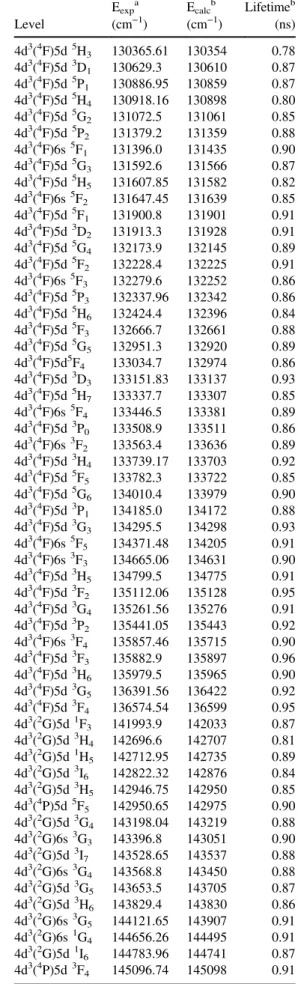
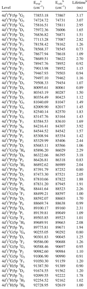
Radiative lifetimes obtained in the present work are reported in table 1 for energy levels belonging to the 4d35d, 4d36s even-parity configurations and in table2for energy levels of the 4d35p, 4d25s5p odd-parity configurations. Unfortunately, no experimental neither theoretical values in MoIII were
previously published in the literature for comparison. How-ever, an argument for assessing the reliability of the present results can be obtained from isoelectronic comparisons, par-ticularly from results obtained recently in NbII (Nilsson
et al 2010), the HFR + CPOL model adopted in this work being the same as that chosen for this isoelectronic ion. More precisely, in this latter work, radiative lifetimes of 17 states belonging to the 4d35p configuration in NbIIwere measured
using the time-resolved laser-inducedfluorescence technique. The comparison of these accurate laboratory measurements with the HFR + CPOL calculations showed that the computed values were in excellent agreement (within 10%) with experimental lifetimes. An excellent agreement (within a few %) was also found when comparing the calculations with the experimental laser spectroscopy measurements obtained by Salih and Lawler (1983) for seven 4d35p levels of NbII.
Consequently, a similar accuracy can also be expected for most of the radiative lifetimes obtained in the present work for MoIII.
Table 1.Calculated radiative lifetimes for levels belonging to the even-parity configurations of MoIII.
Eexpa Ecalcb Lifetimeb
Level (cm−1) (cm−1) (ns) 4d3(4F)5d5H3 130365.61 130354 0.78 4d3(4F)5d3D1 130629.3 130610 0.87 4d3(4F)5d5P1 130886.95 130859 0.87 4d3(4F)5d5H4 130918.16 130898 0.80 4d3(4F)5d5G2 131072.5 131061 0.85 4d3(4F)5d5P2 131379.2 131359 0.88 4d3(4F)6s5F1 131396.0 131435 0.90 4d3(4F)5d5G3 131592.6 131566 0.87 4d3(4F)5d5H5 131607.85 131582 0.82 4d3(4F)6s5F2 131647.45 131639 0.85 4d3(4F)5d5F 1 131900.8 131901 0.91 4d3(4F)5d3D2 131913.3 131928 0.91 4d3(4F)5d5G4 132173.9 132145 0.89 4d3(4F)5d5F2 132228.4 132225 0.91 4d3(4F)6s5F3 132279.6 132252 0.86 4d3(4F)5d5P3 132337.96 132342 0.86 4d3(4F)5d5H6 132424.4 132396 0.84 4d3(4F)5d5F3 132666.7 132661 0.88 4d3(4F)5d5G5 132951.3 132920 0.89 4d3(4F)5d5F 4 133034.7 132974 0.86 4d3(4F)5d3D3 133151.83 133137 0.93 4d3(4F)5d5H7 133337.7 133307 0.85 4d3(4F)6s5F4 133446.5 133381 0.89 4d3(4F)5d3P0 133508.9 133511 0.86 4d3(4F)6s3F2 133563.4 133636 0.89 4d3(4F)5d3H4 133739.17 133703 0.92 4d3(4F)5d5F 5 133782.3 133722 0.85 4d3(4F)5d5G6 134010.4 133979 0.90 4d3(4F)5d3P1 134185.0 134172 0.88 4d3(4F)5d3G3 134295.5 134298 0.93 4d3(4F)6s5F5 134371.48 134205 0.91 4d3(4F)6s3F3 134665.06 134631 0.90 4d3(4F)5d3H5 134799.5 134775 0.91 4d3(4F)5d3F2 135112.06 135128 0.95 4d3(4F)5d3G4 135261.56 135276 0.91 4d3(4F)5d3P 2 135441.05 135443 0.92 4d3(4F)6s3F4 135857.46 135715 0.90 4d3(4F)5d3F3 135882.9 135897 0.96 4d3(4F)5d3H6 135979.5 135965 0.90 4d3(4F)5d3G5 136391.56 136422 0.92 4d3(4F)5d3F4 136574.54 136599 0.95 4d3(2G)5d1F3 141993.9 142033 0.87 4d3(2G)5d3H 4 142696.6 142707 0.81 4d3(2G)5d1H5 142712.95 142735 0.89 4d3(2G)5d3I 6 142822.32 142876 0.84 4d3(2G)5d3H5 142946.75 142950 0.85 4d3(4P)5d5F5 142950.65 142975 0.90 4d3(2G)5d3G4 143198.04 143219 0.88 4d3(2G)6s3G3 143396.8 143051 0.90 4d3(2G)5d3I7 143528.65 143537 0.88 4d3(2G)6s3G4 143568.8 143450 0.88 4d3(2G)5d3G 5 143653.5 143705 0.87 4d3(2G)5d3H6 143829.4 143830 0.86 4d3(2G)6s3G5 144121.65 143907 0.91 4d3(2G)6s1G4 144656.26 144495 0.91 4d3(2G)5d1I6 144783.96 144741 0.87 4d3(4P)5d3F4 145096.74 145098 0.91
4.2. Transition rates
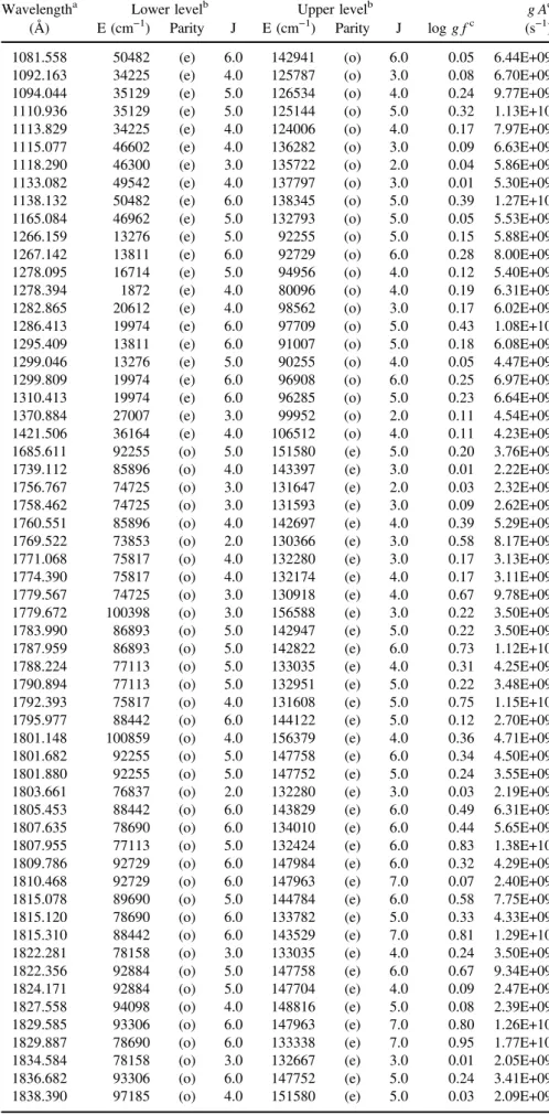
Oscillator strengths and transition probabilities were com-puted for MoIIIspectral lines using our HFR + CPOL model.
Due to space limitations, only a small sample of results cor-responding to the strongest g f-values, i.e. log g f > 0, is presented in table 3. This corresponds to 172 lines in the ultraviolet region from 1081 to 2634 Å. The full set of data containing transition rates for 7555 lines in the wavelength range from extreme ultraviolet to mid-infrared (724 Å–9.32 μm) is reported in table S 3 given as supplementary file (available from …). Note that, in those two tables, the wavelengths (given in vacuum below 2000 Å and in air above that limit) were deduced from experimental energy level values published by Iglesias et al (1990). Laboratory mea-surements of accurate radiative lifetimes and branching frac-tions in MoIIIwould now be welcome to definitely assess the
accuracy of the new theoretical results obtained in the present work. However, in view of the very good agreement observed when comparing available experimental data with our pre-vious calculations performed in many other similar ions using the same HFR + CPOL approach (see reference quoted in the last paragraph of introduction), one can expect uncertainties of the order of 10–20% for the computed transition rates listed in the present paper, at least for the most intense lines.
Acknowledgments
The author is Research Director of the Belgian National Fund for Scientific Research F.R.S.-FNRS. Financial support from this organization is acknowledged.
Table 1. (Continued.) Eexp a Ecalc b Lifetimeb Level (cm−1) (cm−1) (ns) 4d3(2H)5d1H 5 145904.28 145927 0.89 4d3(2H)5d3I7 146257.14 146257 0.87 4d3(2H)5d3I6 146277.52 146260 0.86 4d3(2H)5d3I5 146342.74 146317 0.86 4d3(2D)5d3G4 147431.23 147379 0.88 4d3(2H)6s3H4 147703.6 147730 0.90 4d3(2H)6s3H5 147752.1 147814 0.90 4d3(2H)5d3K 6 147758.2 147753 0.83 4d3(2H)5d3K7 147963.3 147947 0.87 4d3(2H)6s3H6 147984.1 148082 0.90 4d3(2H)5d1K7 148595.3 148584 0.92 4d3(2H)6s1H5 148816.1 148818 0.89 4d3(2H)5d3H5 151580.2 151588 0.84 4d3(2F)6s3F4 156378.82 156256 0.88 4d3(2F)6s3F3 156587.8 156362 0.87 4d3(2F)6s1F3 157546.6 157385 0.92 a From Iglesias et al (1990). b This work.
Table 2.Calculated radiative lifetimes for levels belonging to the odd-parity configurations of MoIII.
Eexpa Ecalcb Lifetimeb
Level (cm−1) (cm−1) (ns) 4d3(4F)5p5G2 73853.18 73867 3.17 4d3(4F)5p5G3 74724.72 74731 3.07 4d3(4F)5p5G4 75816.51 75811 2.95 4d3(4F)5p3D1 75972.36 76006 1.65 4d3(4F)5p3D2 76836.82 76871 1.51 4d3(4F)5p5G5 77113.28 77087 2.82 4d3(4F)5p5F3 78158.42 78162 1.26 4d3(4F)5p5D0 78568.37 78545 0.73 4d3(4F)5p5F1 78677.94 78618 1.09 4d3(4F)5p5G6 78689.51 78622 2.70 4d3(4F)5p5D 1 78947.76 78952 0.92 4d3(4F)5p5F2 79013.98 78952 1.15 4d3(4F)5p5D2 79467.93 79503 0.94 4d3(4F)5p5F4 79497.10 79462 1.16 4d3(4F)5p5D3 79508.33 79454 1.07 4d3(4F)5p5D4 80095.61 80061 0.89 4d3(4F)5p5F5 80343.19 80287 1.50 4d3(4F)5p3D3 80354.49 80423 1.12 4d3(4F)5p3G3 81040.69 81047 1.49 4d3(4F)5p3G 4 82009.90 82017 1.45 4d3(4F)5p3F2 82540.14 82570 1.83 4d3(4F)5p3G5 83147.76 83164 1.43 4d3(4F)5p3F3 83584.53 83610 1.69 4d3(2P)5p1S0 84216.41 84307 3.92 4d3(4F)5p3F4 84544.52 84542 1.57 4d3(4P)5p5P1 85308.94 85354 1.42 4d3(4P)5p3P 2 85329.99 85406 2.44 4d3(4P)5p5D1 85683.11 85566 1.06 4d3(2G)5p3H4 85896.20 86029 2.29 4d3(4P)5p5D0 86322.66 86395 3.18 4d3(4P)5p5P2 86426.81 86318 0.83 4d3(2G)5p3H5 86892.62 86989 2.04 4d3(4P)5p5P3 87391.79 87252 0.80 4d3(4P)5p5D2 87473.30 87521 2.05 4d3(4P)5p5D3 87810.66 87822 1.88 4d3(4P)5p3P 1 87831.20 87945 1.91 4d3(2G)5p3H6 88441.64 88523 2.26 4d3(2G)5p1F3 88499.21 88597 1.00 4d3(2P)5p1D2 88592.07 88603 1.70 4d3(2P)5p3P0 88669.74 88638 0.99 4d3(4P)5p5D4 89100.17 89160 2.31 4d3(2P)5p3P1 89139.81 89049 1.09 4d3(2G)5p3F 4 89503.85 89523 1.01 4d3(2G)5p1H5 89689.91 89663 2.08 4d3(4P)5p3P 0 89775.81 89671 1.94 4d3(2G)5p3G4 90255.05 90292 0.80 4d3(2P)5p3D1 90301.83 90045 1.25 4d3(2G)5p3F2 90586.00 90688 1.26 4d3(2G)5p3G3 90588.46 90697 0.95 4d3(2P)5p3P2 90982.60 90984 1.10 4d3(2G)5p3G5 91006.90 90990 0.91 4d3(2G)5p3F 3 91050.30 91159 1.20 4d3(2H)5p3H4 91387.50 91389 0.90 4d3(2P)5p3D2 91674.55 91562 1.20 4d3(4P)5p5S2 92099.55 92222 1.78 4d3(2H)5p3H5 92254.52 92162 1.02 4d3(2H)5p3H6 92728.95 92619 1.00
Table 2. (Continued.) Eexp a Ecalc b Lifetimeb Level (cm−1) (cm−1) (ns) 4d3(2P)5p3D 3 92758.61 92667 0.98 4d3(2H)5p3I5 92884.18 92841 1.76 4d3(2G)5p1G4 93102.01 93198 1.05 4d3(2P)5p3S1 93222.37 92904 0.94 4d3(2H)5p3I6 93306.10 93224 2.20 4d3(2D)5p3F2 93642.52 93696 0.82 4d3(2D)5p1P1 93709.46 93668 0.81 4d3(2H)5p1G 4 94098.26 94258 1.35 4d3(2D)5p3F3 94117.58 94132 0.80 4d3(2D)5p3D1 94292.66 94396 0.88 4d3(4P)5p3D2 94387.70 94479 0.93 4d3(2H)5p3I7 94424.07 94335 2.47 4d3(4P)5p3D3 94676.73 94698 0.95 4d3(2D)5p3F4 94955.85 94999 0.88 4d3(4P)5p3D1 95016.32 94975 0.88 4d3(2D)5p3D2 95551.80 95534 0.84 4d3(2D)5p3D3 95856.45 95884 1.09 4d3(2H)5p3G5 96285.38 96170 0.68 4d3(2D)5p3P2 96589.89 96592 0.90 4d3(2D)5p3P1 96736.45 96826 0.94 4d3(2H)5p3G3 96838.34 96850 0.79 4d3(2H)5p1I6 96907.92 96762 1.14 4d3(2D)5p3P0 97135.60 97189 0.92 4d3(2H)5p3G 4 97184.77 97192 0.83 4d3(2H)5p1H5 97709.08 97709 0.60 4d3(2D)5p1F3 98562.38 98589 0.68 4d3(2P)5p1P1 99313.02 99336 0.94 4d3(2F)5p3F2 99952.26 99960 0.74 4d3(4P)5p3S1 100184.65 100178 1.06 4d3(2D)5p1D2 100219.97 100213 1.24 4d3(2F)5p3F3 100397.67 100389 1.28 4d3(2F)5p3F4 100858.67 100842 1.30 4d3(2F)5p3G3 102557.67 102504 1.60 4d3(2F)5p3G4 103276.74 103211 1.51 4d3(2F)5p1D2 103303.98 103501 1.14 4d3(2F)5p3G5 103621.4 103536 1.54 4d3(2F)5p3D3 103667.40 103744 1.10 4d3(2F)5p3D2 104511.12 104626 1.07 4d3(2F)5p3D1 105041.26 105175 1.05 4d3(2F)5p1G4 106511.94 106530 1.15 4d3(2F)5p1F3 106803.63 106726 0.90 4d3(2D)5p3D1 114014.74 114042 0.87 4d3(2D)5p3D2 114083.06 114080 0.90 4d3(2D)5p3D3 114591.26 114538 0.90 4d3(2D)5p3F2 115794.02 115799 1.28 4d3(2D)5p3F3 116497.95 116385 1.25 4d3(2D)5p3F4 117287.80 117164 1.38 4d3(2D)5p1D2 117336.75 117392 0.95 4d3(2D)5p3P 2 118451.23 118432 1.21 4d2(3F)5s5p5G2 119170.3 119106 7.73 4d3(2D)5p3P1 119206.22 119230 1.22 4d3(2D)5p1F3 119479.53 119402 1.01 4d3(2D)5p3P0 119559.55 119602 1.22 4d2(3F)5s5p5G3 120064.7 120027 7.27 4d2(3F)5s5p5G4 121118.4 121255 6.94 4d2(3F)5s5p5F1 121723.8 121620 0.90 4d2(3F)5s5p5F2 122229.55 122149 0.90 4d2(3F)5s5p5G5 122817.2 122755 6.82 Table 2. (Continued.) Eexp a Ecalc b Lifetimeb Level (cm−1) (cm−1) (ns) 4d2(3F)5s5p5F 3 123007.56 122959 0.90 4d2(3F)5s5p5F4 124005.8 123990 0.90 4d3(2D)5p1P1 124221.46 124295 0.91 4d2(3F)5s5p5G6 124605.7 124526 8.13 4d2(3F)5s5p5D0 124982.8 125009 0.59 4d2(3F)5s5p5D1 125107.68 125145 0.61 4d2(3F)5s5p5F5 125143.67 125160 0.90 4d2(3F)5s5p5D 2 125359.42 125422 0.63 4d2(3F)5s5p5D3 125786.8 125890 0.66 4d2(3F)5s5p5D4 126533.5 126667 0.64 4d2(3F)5s5p3F2 127336.03 127442 1.79 4d2(3F)5s5p3F3 127795.88 127844 1.52 4d2(3F)5s5p3D2 129055.2 129157 1.05 4d2(3F)5s5p3D1 129065.63 129235 1.11 4d2(3F)5s5p3F4 129383.82 129439 1.54 4d2(3F)5s5p3D3 129964.64 130072 1.10 4d2(3P)5s5p5S2 130073.7 130105 0.61 4d2(3F)5s5p3G3 130453.9 130373 1.22 4d2(3F)5s5p3G4 131570.80 131567 1.14 4d2(3P)5s5p5D1 131782.5 131744 2.35 4d2(3P)5s5p3S1 132164.6 132104 0.86 4d2(3P)5s5p5D2 132439.5 132402 2.08 4d2(3F)5s5p3G5 132792.84 132832 1.13 4d2(3P)5s5p5D 3 133255.4 133143 1.48 4d2(3F)5s5p1D2 133422.2 133372 1.20 4d2(3F)5s5p1F3 133818.4 133760 1.44 4d2(3P)5s5p5D4 134502.10 134420 1.61 4d2(3P)5s5p5P2 134695.4 134824 0.89 4d2(3P)5s5p5P1 134844.9 134869 1.15 4d2(1D)5s5p3F2 135721.81 135589 0.68 4d2(1D)5s5p3P2 135963.7 135956 1.14 4d2(3P)5s5p5P3 136281.5 136182 0.68 4d2(1D)5s5p3P1 136300.2 136373 0.97 4d2(1D)5s5p3F3 136402.5 136321 1.53 4d2(3F)5s5p1G4 136575.7 136451 0.78 4d2(1G)5s5p3G4 137605.1 137524 0.70 4d2(1G)5s5p3G3 137796.5 137777 0.72 4d2(1G)5s5p3G5 138344.9 138162 0.64 4d2(1D)5s5p3F4 138688.1 138672 0.70 4d2(1D)5s5p3D3 139243.0 139257 1.35 4d2(1G)5s5p3H4 141176.2 141222 1.68 4d2(1G)5s5p3H5 141967.4 142045 1.86 4d2(3P)5s5p3D1 142845.9 142974 0.93 4d2(1G)5s5p3H6 142940.8 143056 1.90 a From Iglesias et al (1990). b This work.
Table 3.Oscillator strengths and transition probabilities for strong MoIIIlines (log g f > 0.0).
Wavelengtha Lower levelb Upper levelb g Ac
(Å) E (cm−1) Parity J E (cm−1) Parity J log g fc (s−1)
1081.558 50482 (e) 6.0 142941 (o) 6.0 0.05 6.44E+09
1092.163 34225 (e) 4.0 125787 (o) 3.0 0.08 6.70E+09
1094.044 35129 (e) 5.0 126534 (o) 4.0 0.24 9.77E+09
1110.936 35129 (e) 5.0 125144 (o) 5.0 0.32 1.13E+10
1113.829 34225 (e) 4.0 124006 (o) 4.0 0.17 7.97E+09
1115.077 46602 (e) 4.0 136282 (o) 3.0 0.09 6.63E+09
1118.290 46300 (e) 3.0 135722 (o) 2.0 0.04 5.86E+09
1133.082 49542 (e) 4.0 137797 (o) 3.0 0.01 5.30E+09
1138.132 50482 (e) 6.0 138345 (o) 5.0 0.39 1.27E+10
1165.084 46962 (e) 5.0 132793 (o) 5.0 0.05 5.53E+09
1266.159 13276 (e) 5.0 92255 (o) 5.0 0.15 5.88E+09
1267.142 13811 (e) 6.0 92729 (o) 6.0 0.28 8.00E+09
1278.095 16714 (e) 5.0 94956 (o) 4.0 0.12 5.40E+09
1278.394 1872 (e) 4.0 80096 (o) 4.0 0.19 6.31E+09
1282.865 20612 (e) 4.0 98562 (o) 3.0 0.17 6.02E+09
1286.413 19974 (e) 6.0 97709 (o) 5.0 0.43 1.08E+10
1295.409 13811 (e) 6.0 91007 (o) 5.0 0.18 6.08E+09
1299.046 13276 (e) 5.0 90255 (o) 4.0 0.05 4.47E+09
1299.809 19974 (e) 6.0 96908 (o) 6.0 0.25 6.97E+09
1310.413 19974 (e) 6.0 96285 (o) 5.0 0.23 6.64E+09
1370.884 27007 (e) 3.0 99952 (o) 2.0 0.11 4.54E+09
1421.506 36164 (e) 4.0 106512 (o) 4.0 0.11 4.23E+09
1685.611 92255 (o) 5.0 151580 (e) 5.0 0.20 3.76E+09
1739.112 85896 (o) 4.0 143397 (e) 3.0 0.01 2.22E+09
1756.767 74725 (o) 3.0 131647 (e) 2.0 0.03 2.32E+09
1758.462 74725 (o) 3.0 131593 (e) 3.0 0.09 2.62E+09
1760.551 85896 (o) 4.0 142697 (e) 4.0 0.39 5.29E+09
1769.522 73853 (o) 2.0 130366 (e) 3.0 0.58 8.17E+09
1771.068 75817 (o) 4.0 132280 (e) 3.0 0.17 3.13E+09
1774.390 75817 (o) 4.0 132174 (e) 4.0 0.17 3.11E+09
1779.567 74725 (o) 3.0 130918 (e) 4.0 0.67 9.78E+09
1779.672 100398 (o) 3.0 156588 (e) 3.0 0.22 3.50E+09
1783.990 86893 (o) 5.0 142947 (e) 5.0 0.22 3.50E+09
1787.959 86893 (o) 5.0 142822 (e) 6.0 0.73 1.12E+10
1788.224 77113 (o) 5.0 133035 (e) 4.0 0.31 4.25E+09
1790.894 77113 (o) 5.0 132951 (e) 5.0 0.22 3.48E+09
1792.393 75817 (o) 4.0 131608 (e) 5.0 0.75 1.15E+10
1795.977 88442 (o) 6.0 144122 (e) 5.0 0.12 2.70E+09
1801.148 100859 (o) 4.0 156379 (e) 4.0 0.36 4.71E+09
1801.682 92255 (o) 5.0 147758 (e) 6.0 0.34 4.50E+09
1801.880 92255 (o) 5.0 147752 (e) 5.0 0.24 3.55E+09
1803.661 76837 (o) 2.0 132280 (e) 3.0 0.03 2.19E+09
1805.453 88442 (o) 6.0 143829 (e) 6.0 0.49 6.31E+09
1807.635 78690 (o) 6.0 134010 (e) 6.0 0.44 5.65E+09
1807.955 77113 (o) 5.0 132424 (e) 6.0 0.83 1.38E+10
1809.786 92729 (o) 6.0 147984 (e) 6.0 0.32 4.29E+09
1810.468 92729 (o) 6.0 147963 (e) 7.0 0.07 2.40E+09
1815.078 89690 (o) 5.0 144784 (e) 6.0 0.58 7.75E+09
1815.120 78690 (o) 6.0 133782 (e) 5.0 0.33 4.33E+09
1815.310 88442 (o) 6.0 143529 (e) 7.0 0.81 1.29E+10
1822.281 78158 (o) 3.0 133035 (e) 4.0 0.24 3.50E+09
1822.356 92884 (o) 5.0 147758 (e) 6.0 0.67 9.34E+09
1824.171 92884 (o) 5.0 147704 (e) 4.0 0.09 2.47E+09
1827.558 94098 (o) 4.0 148816 (e) 5.0 0.08 2.39E+09
1829.585 93306 (o) 6.0 147963 (e) 7.0 0.80 1.26E+10
1829.887 78690 (o) 6.0 133338 (e) 7.0 0.95 1.77E+10
1834.584 78158 (o) 3.0 132667 (e) 3.0 0.01 2.05E+09
1836.682 93306 (o) 6.0 147752 (e) 5.0 0.24 3.41E+09
Table 3. (Continued.)
Wavelengtha Lower levelb Upper levelb g Ac
(Å) E (cm−1) Parity J E (cm−1) Parity J log g fc (s−1)
1842.123 79497 (o) 4.0 133782 (e) 5.0 0.40 4.90E+09
1845.715 78158 (o) 3.0 132338 (e) 3.0 0.05 2.19E+09
1847.081 89690 (o) 5.0 143829 (e) 6.0 0.20 3.11E+09
1850.882 80343 (o) 5.0 134371 (e) 5.0 0.54 6.76E+09
1851.063 92255 (o) 5.0 146278 (e) 6.0 0.33 4.16E+09
1853.589 79497 (o) 4.0 133447 (e) 4.0 0.31 3.92E+09
1856.994 89100 (o) 4.0 142951 (e) 5.0 0.66 8.87E+09
1857.128 89100 (o) 4.0 142947 (e) 5.0 0.11 2.50E+09
1859.529 91007 (o) 5.0 144784 (e) 6.0 0.32 4.02E+09
1863.335 80343 (o) 5.0 134010 (e) 6.0 0.60 7.69E+09
1867.064 94424 (o) 7.0 147984 (e) 6.0 0.40 4.78E+09
1868.175 92729 (o) 6.0 146257 (e) 7.0 0.49 5.93E+09
1872.893 92884 (o) 5.0 146278 (e) 6.0 0.27 3.58E+09
1874.383 80096 (o) 4.0 133447 (e) 4.0 0.02 1.99E+09
1875.692 94118 (o) 3.0 147431 (e) 4.0 0.21 3.09E+09
1875.783 103277 (o) 4.0 156588 (e) 3.0 0.05 2.10E+09
1877.765 81041 (o) 3.0 134296 (e) 3.0 0.10 2.36E+09
1877.876 82010 (o) 4.0 135262 (e) 4.0 0.19 2.93E+09
1878.153 83148 (o) 5.0 136392 (e) 5.0 0.30 3.74E+09
1878.261 93102 (o) 4.0 146343 (e) 5.0 0.26 3.42E+09
1881.171 79508 (o) 3.0 132667 (e) 3.0 0.13 2.55E+09
1885.973 89690 (o) 5.0 142713 (e) 5.0 0.34 4.11E+09
1886.077 92884 (o) 5.0 145904 (e) 5.0 0.24 3.30E+09
1887.493 90588 (o) 3.0 143569 (e) 4.0 0.09 2.27E+09
1887.810 93306 (o) 6.0 146278 (e) 6.0 0.42 4.93E+09
1888.537 93306 (o) 6.0 146257 (e) 7.0 0.22 3.14E+09
1888.824 90255 (o) 4.0 143198 (e) 4.0 0.38 4.44E+09
1891.944 80096 (o) 4.0 132951 (e) 5.0 0.49 5.75E+09
1892.802 83148 (o) 5.0 135980 (e) 6.0 0.76 1.07E+10
1893.133 91007 (o) 5.0 143829 (e) 6.0 0.30 3.68E+09
1893.640 90588 (o) 3.0 143397 (e) 3.0 0.07 2.13E+09
1894.035 80354 (o) 3.0 133152 (e) 3.0 0.12 2.47E+09
1894.313 82010 (o) 4.0 134800 (e) 5.0 0.71 9.58E+09
1895.468 103621 (o) 5.0 156379 (e) 4.0 0.16 2.69E+09
1896.304 91388 (o) 4.0 144122 (e) 5.0 0.18 2.79E+09
1897.184 83148 (o) 5.0 135857 (e) 4.0 0.19 2.83E+09
1897.588 81041 (o) 3.0 133739 (e) 4.0 0.65 8.27E+09
1898.774 79508 (o) 3.0 132174 (e) 4.0 0.48 5.55E+09
1899.149 82010 (o) 4.0 134665 (e) 3.0 0.13 2.51E+09
1899.458 91007 (o) 5.0 143654 (e) 5.0 0.38 4.46E+09
1901.914 79014 (o) 2.0 131593 (e) 3.0 0.33 3.92E+09
1902.156 82540 (o) 2.0 135112 (e) 2.0 0.18 2.76E+09
1903.938 81041 (o) 3.0 133563 (e) 2.0 0.03 1.97E+09
1906.291 90255 (o) 4.0 142713 (e) 5.0 0.28 3.52E+09
1912.105 83585 (o) 3.0 135883 (e) 3.0 0.37 4.27E+09
1914.156 80096 (o) 4.0 132338 (e) 3.0 0.08 2.21E+09
1921.967 84545 (o) 4.0 136575 (e) 4.0 0.55 6.45E+09
1925.304 91007 (o) 5.0 142947 (e) 5.0 0.06 2.07E+09
1926.479 96908 (o) 6.0 148816 (e) 5.0 0.43 4.81E+09
1928.750 84545 (o) 4.0 136392 (e) 5.0 0.56 6.50E+09
1929.270 94424 (o) 7.0 146257 (e) 7.0 0.56 6.55E+09
1930.278 94098 (o) 4.0 145904 (e) 5.0 0.15 2.49E+09
1932.167 82540 (o) 2.0 134296 (e) 3.0 0.24 3.11E+09
1934.708 96908 (o) 6.0 148595 (e) 7.0 0.89 1.40E+10
1935.096 83585 (o) 3.0 135262 (e) 4.0 0.33 3.79E+09
1945.802 92729 (o) 6.0 144122 (e) 5.0 0.17 2.59E+09
1959.453 106512 (o) 4.0 157547 (e) 3.0 0.15 2.43E+09
1968.516 92729 (o) 6.0 143529 (e) 7.0 0.33 3.69E+09
Table 3. (Continued.)
Wavelengtha Lower levelb Upper levelb g Ac
(Å) E (cm−1) Parity J E (cm−1) Parity J log g fc (s−1)
1977.561 97185 (o) 4.0 147752 (e) 5.0 0.07 2.01E+09
1983.340 94677 (o) 3.0 145097 (e) 4.0 0.33 3.58E+09
2074.234 97709 (o) 5.0 145904 (e) 5.0 0.09 1.92E+09
2113.644 49542 (e) 4.0 96838 (o) 3.0 0.03 1.62E+09
2133.072 50319 (e) 5.0 97185 (o) 4.0 0.20 2.32E+09
2170.584 33452 (e) 3.0 79508 (o) 3.0 0.06 1.63E+09
2179.381 34225 (e) 4.0 80096 (o) 4.0 0.02 1.48E+09
2182.544 50482 (e) 6.0 96285 (o) 5.0 0.06 1.58E+09
2184.304 46962 (e) 5.0 92729 (o) 6.0 0.09 1.72E+09
2190.445 43462 (e) 3.0 89100 (o) 4.0 0.23 2.35E+09
2211.028 35129 (e) 5.0 80343 (o) 5.0 0.26 2.47E+09
2214.400 42666 (e) 2.0 87811 (o) 3.0 0.10 1.72E+09
2216.611 72188 (e) 3.0 117288 (o) 4.0 0.36 3.11E+09
2224.649 58730 (e) 4.0 103667 (o) 3.0 0.01 1.37E+09
2226.929 58730 (e) 4.0 103621 (o) 5.0 0.43 3.63E+09
2252.421 58894 (e) 3.0 103277 (o) 4.0 0.30 2.63E+09
2253.197 35129 (e) 5.0 79497 (o) 4.0 0.18 1.97E+09
2257.204 46300 (e) 3.0 90588 (o) 3.0 0.05 1.49E+09
2264.742 72356 (e) 2.0 116498 (o) 3.0 0.22 2.14E+09
2269.714 46962 (e) 5.0 91007 (o) 5.0 0.22 2.13E+09
2275.001 50482 (e) 6.0 94424 (o) 7.0 0.62 5.40E+09
2275.488 34225 (e) 4.0 78158 (o) 3.0 0.05 1.44E+09
2275.637 43462 (e) 3.0 87392 (o) 3.0 0.06 1.45E+09
2289.202 49089 (e) 2.0 92759 (o) 3.0 0.03 1.36E+09
2290.062 46602 (e) 4.0 90255 (o) 4.0 0.09 1.55E+09
2294.974 35129 (e) 5.0 78690 (o) 6.0 0.58 4.80E+09
2296.561 51426 (e) 3.0 94956 (o) 4.0 0.27 2.32E+09
2298.245 59060 (e) 2.0 102558 (o) 3.0 0.14 1.74E+09
2306.494 49542 (e) 4.0 92884 (o) 5.0 0.05 1.41E+09
2325.556 50319 (e) 5.0 93306 (o) 6.0 0.51 3.98E+09
2330.945 34225 (e) 4.0 77113 (o) 5.0 0.40 3.09E+09
2332.694 54853 (e) 5.0 97709 (o) 5.0 0.03 1.31E+09
2349.913 46962 (e) 5.0 89504 (o) 4.0 0.02 1.26E+09
2353.747 64331 (e) 3.0 106804 (o) 3.0 0.16 1.72E+09
2357.584 72188 (e) 3.0 114591 (o) 3.0 0.22 2.00E+09
2359.758 33452 (e) 3.0 75817 (o) 4.0 0.26 2.20E+09
2366.290 50482 (e) 6.0 92729 (o) 6.0 0.28 2.28E+09
2370.025 64331 (e) 3.0 106512 (o) 4.0 0.19 1.83E+09
2372.982 58730 (e) 4.0 100859 (o) 4.0 0.29 2.28E+09
2377.137 54853 (e) 5.0 96908 (o) 6.0 0.49 3.63E+09
2383.876 50319 (e) 5.0 92255 (o) 5.0 0.24 2.02E+09
2384.649 77557 (e) 2.0 119480 (o) 3.0 0.18 1.75E+09
2386.965 32843 (e) 2.0 74725 (o) 3.0 0.13 1.57E+09
2408.682 58894 (e) 3.0 100398 (o) 3.0 0.10 1.46E+09
2410.094 46962 (e) 5.0 88442 (o) 6.0 0.33 2.43E+09
2474.252 52698 (e) 4.0 93102 (o) 4.0 0.12 1.44E+09
2481.192 46602 (e) 4.0 86893 (o) 5.0 0.22 1.79E+09
2487.664 52698 (e) 4.0 92884 (o) 5.0 0.00 1.09E+09
2490.018 49542 (e) 4.0 89690 (o) 5.0 0.00 1.08E+09
2506.187 44655 (e) 4.0 84545 (o) 4.0 0.22 1.78E+09
2524.709 46300 (e) 3.0 85896 (o) 4.0 0.19 1.63E+09
2547.336 54853 (e) 5.0 94098 (o) 4.0 0.04 1.14E+09
2597.134 44655 (e) 4.0 83148 (o) 5.0 0.18 1.50E+09
2633.565 50482 (e) 6.0 88442 (o) 6.0 0.11 1.25E+09
a
Wavelengths deduced from experimental energies reported by Iglesias et al (1990).
b
Iglesias et al (1990).
c
References
Baumann M, Liening H and Lindel H 1978 Phys. Lett. A68 319 Biémont E et al 2005 Proc. SPIE5830 221
Biémont E et al 2011 Mon. Not. R. Astron. Soc.414 3350 Campos J et al 2005 Mon. Not. R. Astron. Soc.363 905 Cowan R D 1981 The Theory of Atomic Structure and Spectra
(Berkeley, CA: University of California Press)
Dickerman P J and Deuel R W 1964 J. Quant. Spectrosc. Radiat. Transfer4 807
Duquette D W, Salih S and Lawler J E 1981 Phys. Lett. A83 214 Fivet V et al 2009 Mon. Not. R. Astron. Soc.396 2124
Fraga S, Karwowski J and Saxena K M S 1976 Handbook of Atomic Data (Amsterdam: Elsevier)
Hannaford P and Lowe R M 1983 J. Phys. B: At. Mol. Phys.16 4539 Hartman H et al 2010 Phys. Rev. A82 052512
Iglesias L, Cabeza M I and Kaufman V 1990 J. Res. Natl Inst. Stand. Technol.95 647
Iglesias L, Cabeza M I, Rico F R and Kaufman V 1988 Phys. Scr.
37 855
Jiang L Y et al 2012 Eur. Phys. J. D66 176 Jiang L Y et al 2013 J. Opt. Soc. Am. B30 489
Kwiatkowski M, Micali G, Werner K and Zimmermann P 1981 Phys. Lett. A85 273
Lipschultz B et al 2006 Phys. Plasmas13 056117 Liu Z X et al 2013 Nucl. Fusion53 073041
Lundberg H et al 2010 J. Phys. B: At. Mol. Opt. Phys.43 085004 Malcheva G et al 2006 Mon. Not. R. Astron. Soc.367 754
Malcheva G et al 2011 Mon. Not. R. Astron. Soc.412 1823 Nilsson H et al 2010 Astron. Astrophys.511 A16
Palmeri P and Wyart J-F 1998 Phys. Scr.58 445 Palmeri P et al 2007 Mon. Not. R. Astron. Soc.374 63 Palmeri P et al 2009 J. Phys. B: At. Mol. Opt. Phys.42 165005 Peterson R C 2011 Astrophys. J742 21
Peterson R C 2013 Astrophys. J. Lett.768 L13 Quinet P 2002 J. Phys. B: At. Mol. Opt. Phys.35 19 Quinet P et al 1999 Mon. Not. R. Astron. Soc.307 934 Quinet P et al 2002 J. Alloys Compd.344 255
Quinet P et al 2011 J. Electron Spectrosc. Relat. Phenom.184 174 Quinet P et al 2012 Astron. Astrophys.537 A74
Salih S and Lawler J E 1983 Phys. Rev. A28 3653
Schnehage S E, Danzmann K, Künnemeyer R and Kock M 1983 J. Quant. Spectrosc. Radiat. Transfer29 507
Sikström et al 2001 J. Phys. B: At. Mol. Opt. Phys.34 477 Whaling W 1984 J. Quant. Spectrosc. Radiat. Transfer32 69 Whaling W 1986 J. Quant. Spectrosc. Radiat. Transfer36 491 Whaling W and Brault J W 1988 Phys. Scr.38 707
Xu H L et al 2006 Astron. Astrophys.452 357 Zhang Y et al 2008 Phys. Rev. A78 022505 Zhang W et al 2009 Eur. Phys. J. D55 1
Zhang W et al 2010 J. Phys. B: At. Mol. Opt. Phys.43 205005 Zhang W, Palmeri P and Quinet P 2013 Phys. Scr.88 065302 Zhang W, Palmeri P, Quinet P and Biémont E 2013 Astron.
Astrophys.551 A136
QUERY FORM
J
OURNAL:
Physica Scripta
A
UTHOR:
P Quinet
T
ITLE:
Atomic structure, radiative lifetime and oscillator strength calculations in doubly ionized
molybdenum (Mo
III)
A
RTICLEID:
ps504644
The layout of this article has not yet beenfinalized. Therefore this proof may contain columns that are not fully balanced/ matched or overlapping text in inline equations; these issues will be resolved once thefinal corrections have been incorporated.