Deliverable D2.4
Scenario 3: Medium-case
30/11/2017
BRAIN-TRAINS
Transversal assessment of new
intermodal strategies
WP2: Optimal corridor and hub development
Christine Tawfik and Sabine Limbourg - QuantOM (HEC-ULg)
BELGIAN RESEARCH ACTION THROUGH
INTERDISCIPLINARY NETWORKS
CONTENTS
CONTENTS ... 2 INTRODUCTION ... 3 1. HYPOTHESES ... 4 1.1 Scenario parameters ... 41.2 Other operational parameters ... 5
2. MODELLING APPROACH ... 6
2.1 Service network design... 6
2.2 Generalized costs... 7
2.3 Costs’ weights estimation ... 7
3. RESULTS AND DISCUSSION ... 9
3.1 Service network design – National flows ... 9
3.2 Generalized costs – RailNetEurope corridors ... 12
4. CONCLUSIONS ... Error! Bookmark not defined. REFERENCES ... 16
INTRODUCTION
WP2: Optimal corridor and hub development aims at providing tools from the operations research domain, in order to highlight the potential efficiency of intermodal rail transport in Belgium. The objective of this package is also to give more insight on the decision-making process of the different stakeholders in the intermodal transport chain. The methods are based on the area of expertise of optimization, which aims at translating a managerial problem into a mathematical model that should be optimized. The main components of the methodology consist in:
1) Identifying the managerial problem,
2) Modelling the problem using mathematical programming, 3) Computing the solutions, and
4) Translating the scenarios.
As previously defined in deliverable D1.3, the general goal of the scenarios, within the present research context, is to identify the impact of different plausible situations on the future development of intermodal rail transport, principally in Belgium. The difference between offering insights into the future, the main scope of the developed scenarios, and attempting to forecast its exact nature is specially highlighted.
As far as WP2 is concerned, the aim is to provide guidelines and outlooks as to the effect of certain operational factors on the competitiveness and the future success of intermodal transport, measured in agreed upon and quantified terms. Indeed, in previous deliverables, the project proposed different important parameters to consider when dealing with intermodal and rail transport in Belgium. These parameters were retrieved out of a SWOT analysis, and selected based on their relevance and plausibility by a panel of experts, using the so-called Delphi method. Different values have been assigned to each parameter, according to the scenario that is used (best-case, worst-(best-case, middle-case).
As a continuation to the two previous deliverables D2.2 and D2.3, depicting the best and worst-case scenarios respectively, we carry on through this document with the last scenario corresponding to the middle case. The results are based on an operational costs’ analysis regarding offering intermodal services with respect to all-road/trucking services. Different instrumental changes (such as, imposing road taxes and offering rail subsidies) are tested and compared against each other in the middle-case scenario and against the reference scenario to identify the most powerful of them or the combination thereof. The analysis is conducted within an optimization framework extending classical service network design models. Having Belgium as a study case of interest, the tests are invoked over real aggregated data within Belgium and the European rail freight corridors passing through it. In what follows, we elaborate on the elements considered for the scenario analysis, the underlying mathematical model, the obtained results for the middle-case scenario and the corresponding differences with respect to the reference case. We conclude with a
discussion of the effectiveness of the instrumental changes and the main recommendations in light of the desired perspectives of the research.
1. HYPOTHESES
1.1.
Scenario parameters
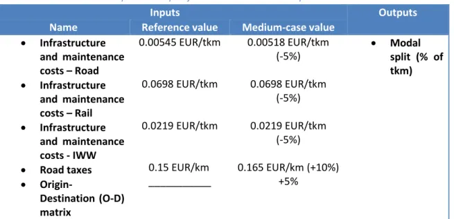
The scenarios are designed in a direct linkage to the goals set by the White Paper on transport from the European Commission (2011): principally achieving a 30% road freight shift by the year 2030, adopted by the transport stakeholders. Contrary to the two previous relatively extreme cases, the medium-case scenario is considered as an in-between scenario, where the White Paper goals are still carried on from the best case, however not required to be completely reached by 2030. A partial achievement represented in a fractional shift from road to intermodal transport would be accepted. Based on the realized SWOT analysis for each WP, the results are translated into a selection of crucial scenario elements and corresponding parameters and values, validated by the panel of experts of the BRAIN-TRAINS project. In light of this perspective, able 1 shows the considered inputs and outputs for WP2, among the total list of scenario parameters, together with the calculated reference- and medium-case values of the inputs.
Table 1: Inputs and outputs from the considered scenario parameters
Inputs Outputs
Name Reference value Medium-case value
Infrastructure and maintenance costs – Road Infrastructure and maintenance costs – Rail Infrastructure and maintenance costs - IWW Road taxes Origin-Destination (O-D) matrix 0.00545 EUR/tkm 0.0698 EUR/tkm 0.0219 EUR/tkm 0.15 EUR/km ___________ 0.00518 EUR/tkm (-5%) 0.0698 EUR/tkm (-5%) 0.0219 EUR/tkm (-5%) 0.165 EUR/km (+10%) +5% Modal split (% of tkm)
SOURCE:OWN COMPOSITION, BASED ON DELIVERABLE D1.3
The infrastructure and maintenance costs, as stated in CE Delft (2010) comprise: the construction costs, the maintenance and operational costs and the land use costs. The study further provides a fixed and variable parts division of the costs for each of the considered transport modes, i.e. road, rail and inland waterways (IWW). The reference road taxes values are calculated based on the updated values of the Viapass tax in Belgium, corresponding to the average existing rates weighed by the number of vehicles in each category for 2014 (Emisia, 2015).
1.2.
Other operational parameters
In addition to the above stated parameters, other elements are considered as well to establish necessary operational hypotheses and elements throughout the model runs. The values are based on the norms applied in real life situations according to the collected industry information. Table 2 presents those input parameters that were not explicitly stated among the scenario elements, their selected values (where applicable), as well as additional calculated outputs.
Table 2: Additional operational inputs and outputs
Inputs Outputs
Name Value
Truck capacity 24 tonnes
Train capacity 1500 tonnes
IWW vessel capacity 3000 tonnes
Truck av. speed 45 km/h (short haul)
Truck av. speed 70 km/h (long haul)
Train av. speed 90 km/h
Vessel av. speed 12 km/h
Transhipment time 200 s/container
Intermodal market share Intermodal services’ frequencies (per week) Intermodal itineraries (demands’ routing) SOURCE:OWN COMPOSITION
As for the stated modes’ speeds, average cases are assumed for simplification purposes, while acknowledging the existing speed variances in terms of the chosen connections and travelled regions. This is especially valid for the rail freight part; for instance, on the Scandinavian-Mediterranean rail corridor, a requirement is set to attain an operating speed of 100 km/h. However, some sections in Austria only allow 80 km/h due to mountain rail operations. Other speed restrictions for wider bundle of sections are experienced in Italy as well (European Commission, 2014). Furthermore, an assumption is made that freight trains are principally scheduled during the night, hence face low congestion levels. Transhipment times are estimated as well based on previous statistics shared by sample terminals in Europe (e.g. Port of Rotterdam) and assumed for the worst cases.
Another important parameter to take into account is the location of the terminals. At the domestic level of Belgium, the locations are aggregated to the third level of the Nomenclature of Territorial Units for Statistics (NUTS 3), based on the setup by Macharis et al. (2009). Second, at the European level, the terminals’ locations are considered at NUTS 2 level and verified by the Agora’s Europe Database.
2. MODELLING APPROACH
Our methods are based on the concepts of Mathematical Programming, which aims at translating a managerial problem into a mathematical model, within an optimization framework. We address a tactical, medium-term decision horizon, from an economic perspective (i.e.: no environmental impact involved). The decision maker is namely a transport operator/service provider. In this section, we elaborate on the particulars of the underlying mathematical model.
2.1.
Service network design
In order to gain insights about the costs influence on the partition of the flows over the modes of transport in the network, we start by considering a tactical intermodal service network design problem, from the perspective of a transport service provider operating on a road-rail-IWW network. The decisions to be taken are two-fold: (1) the frequencies of the services over a certain period of time, typically a week; (2) optimal demands’ routing over the service network in the form of offered itineraries. A static case is assumed, where the demands are fixed, as well as the underlying physical network, including the terminals’ locations, throughout the decision process. A mixed integer mathematical program (MIP) is considered in the interest of operating costs’ minimization: a reasonable primary objective for both freight carriers and clients. The formulation extends the classical static path-based multicommodity formulation, originally introduced by Crainic (2000) in the general freight transport context and Crainic and Kim (2007) for intermodal transport.
More precisely, we consider as starting inputs a set of shipping demands (alternatively, commodities) that are traveling over the network, each of which is defined by: an origin point, a destination point and the total demand volumes in tonnes. In this context, a service is also defined by its origin point, destination point and transport mode. At a pre-processing stage, a set of admissible intermodal itineraries are generated for each commodity shipping demand, where each itinerary is formed as a combination of services. Admissibility is meant in the sense of being geographically feasible and conforming to the norms of intermodal paths’ structure (i.e. the long haul is performed by non-road modes considering that boundaries on the distance are covered by trucking within an itinerary and the intermodal distance is not considerably larger than the all-road one). The model depicts an objective that minimizes the sum of the following:
- The fixed costs of running each service during the planning period,
- and the variable costs of transporting the goods over the services;
with the fixed costs’ parameters being taken from Table 1, according to each considered mode of transport. Furthermore, the model ensures that the following constraints are strictly respected:
- The total shipping demands should be satisfied and/or delivered by the offered
itineraries.
- An itinerary is not to be used, unless a certain fraction of the demand (e.g., 20%) is sent
over it to enforce a minimum utilization of the itinerary.
We shall refer to this version of the model as SND (Service Network Design) in the remainder of the document.
2.2.
Generalized costs
In completion to the above model, an extension has been developed to account for service quality aspects, principally, the transit time. To better represent this goal, the model builds upon the previous formulation to represent a scheduled service network design problem, prescribing the day for each service dispatch and ensuring a balance of resources at the terminals based on the network design models with asset management discussed in Andersen et al. (2009).
In this formulation, a service will be further defined by its dispatch day, referring to each day of the week. The services’ frequencies will be limited to – at most - one service per day. In addition to the carried on constraints from the previous model, we impose further constraints in order to represent the resources balancing requirement over long corridors. These constraints ensure that each dispatched long haul service will have to be indeed returned to its departure point, using the same train/vessel and being dispatched on the following day of the original service’s arrival. Finally, we consider the total transit time of each itinerary as the sum of the line duration and the transhipment delay at the terminals, including the time needed for the equipment to become available. Consequently, the objective is being updated to denote the minimization of both the out-of-pocket costs and the costs related to the incurred transit time. In order for these components to
yield a consistent monetary output, corresponding mapping weights 𝛽𝑐𝑜𝑠𝑡𝑠 and 𝛽𝑡𝑟𝑎𝑛𝑠𝑖𝑡 are assigned
to each part of the objective.
We shall refer to this version of the model from this point onwards as SND-GC (Service Network Design-Generalized Costs).
2.3.
Costs’ weights estimation
In order to depict realistic values for the weighting parameters in the costs’ minimization objective, we estimate based on a statistical approach the relative importance of each of the considered components in actual practices. To achieve this purpose, a database has been collected based on individual phone interviews, e-mails and internet surveying questionnaires among intermodal transport users in Belgium. It was ensured that it was generally feasible for the respondents to use trucking or intermodal transport either for long haul deliveries or to reach the ports to accomplish a journey of maritime transport. The respondents were approached in the context of a Revealed Preference (RP) survey, in which they were asked to share their effectuated choices in relation to actual situations. More precisely, client firms of container transport were interviewed about time-average statistics for some of their specific origin-destination (O-D) connections, in order to reflect the effect of the network characteristics uniquely. Additionally, shipper-specific information is elicited with respect to the firms' business behavior, corridors' and shipped products' requirements, as well as the mode alternatives' attributes. A total of 101 answers were returned from shipping firms whose annual tonnage ranges from 2000 to 10000 tonnes. Table 3 summarizes the modal share results. Moreover, the following figures are deduced from the
obtained data and further testify the currently challenged position of intermodal transport in the market:
Average freight rate increase of intermodal with respect to all-road transport: 28.2%.
Average transit time increase of intermodal with respect to all-road transport:
98-185.7%.
Average number of days equipment remain unavailable in all-road transport: 3 days.
Average number of days equipment remain unavailable in intermodal transport: 6 days.
Out of the entire 101 sample observations, 60 were further kept on as consistent and complete for the rest of the estimation process.
Table 3: All-road demands’ share with respect to intermodal transport
All-road share Number of
observations <20% 10 20-60% 3 60-90% 6 90-100% 82 Total 101 SOURCE:OWN COMPOSITION
We consider a mathematical expression of the total logistics costs based on the one provided by Vieira (1992). A deterministic case is assumed regarding the probability of reaching a stock-out situation at the destination, in which the transit times and final consumer's demands are fixed. The estimation results are obtained using the freeware Biogeme offered by Bierlaire (2003), developed for the purposes of maximum likelihood estimation of parametric models. For freight
mode 𝑖, let 𝑇𝑖 denote the tariff in monetary units per tonne, 𝑑𝑖 the transit time and 𝑛𝑖 the average
period necessary equipment remained unavailable. We additionally refer to 𝑄 as the annual tonnage shipped by the firm. We show in Table 4 the coefficients’ results associated with the selected costs
attributes based on their statistical significance at the 95th percentile, as indicated by the values of
the t-statistics. The capital carrying costs include the cost of capital tied up during the transit and due to the unavailability of transport equipment.
In the considered context, 𝛽𝑐𝑜𝑠𝑡𝑠 is regarded as a scaling parameter, while 𝛽𝑡𝑟𝑎𝑛𝑠𝑖𝑡 is
behaviorally interpreted as the discount rate per unit of weight and time. All coefficients have the correct sign. The estimation results show that the shippers in our surveyed market accord a relatively high weight to the capital carrying costs, in comparison to the direct out-of-pocket charges: an impression that was primarily shared since the early stages of the survey. The obtained estimation results are ultimately considered as the values of the costs weighting parameters in the generalized costs objective of the above SND-GC model.
Table 4: Estimation results of the logistics costs
Coefficient Estimation results
Associated term Value Standard error t-test
Transport charges - 𝜷𝒄𝒐𝒔𝒕𝒔 T
i
Q 365
-0.0059 0.00259 -2.28
Capital carrying costs - 𝜷𝒕𝒓𝒂𝒏𝒔𝒊𝒕 d
i Q 365+ ni Q 365 -0.00801 0.00408 -1.97 Objective at convergence -27.310 𝝆𝟐 0.283 Adjusted 𝝆𝟐 0.230 SOURCE:OWN COMPOSITION
3. RESULTS AND DISCUSSION
We consider two cases of input data for our operational costs analysis. First, at the domestic level, only freight flows within Belgium are considered, in addition to the sea flows originating from or leaving the country at maritime ports, based on the accessible Worldnet database (Newton, 2009) at the third level of the Nomenclature of Territorial Units for Statistics (NUTS 3). This data set will be referred to through the remainder of the document as Instance 1. Second, at the European level, three further instances are defined based on the geographical information provided by RailNetEurope about the rail freight corridors passing through Belgium (Figure 1), as the market point of interest in our study: namely, the Rhine-Alpine (instance 2), the North Sea-Mediterranean (instance 3) and the North Sea-Baltic (instance 4) corridor. The demands data for the latter case are obtained from Carreira et al. (2012) at the NUTS 2 level, also based on the Worldnet database for Europe. In this section, we shall show the effects of certain parameters’ changes on the intermodal market share, and consequent modal split according to reference- and medium-case scenario developments.
3.1.
Service network design – National flows:
Starting from an O-D matrix of Belgium comprising 357 commodities/shipping demands, all-road paths are enabled for each O-D pair. Different scenario elements are changed to their medium-case values in order to draw conclusion on the flows partition on the different transport modes, if the costs of operating services become the only considered choice criterion. For this experiment, we consider the first version of the model SVN, comprising only out-of-pocket costs, three modes of transport (road, rail and IWWs) and Instance 1 as input data. The first row in Table 5 shows the result when all the parameters are tuned to the reference scenario. In the subsequent rows, we refer to the parameter whose value is changed to the medium-case scenario values, in order to test the effect and significance of each parameter separately; in this case, only the road taxes and demands’ variation will be tested separately as the costs undergo negligible change from the reference to the medium case. At the last row, all parameters’ values follow those defined in the medium-case scenario.
Figure 1: Rail freight corridors in Europe: Corridor 1, 2 and 8
SOURCE:RAILNETEUROPE (2017)
Table 5: Influence of the medium-case parameter values on the national flows’ repartition (Instance 1)
Modified parameter % of freight on intermodal paths % of freight on all-road paths Modal split (% of tkm)
Road Rail IWW
None (reference) 28.44 71.56 78.04 0 21.96
Road taxes 32.98 67.02 73.96 0 26.04
O-D matrix 29.84 70.16 76.92 0 23.08
All (Medium-case) 32.29 67.71 74.44 0 25.56
SOURCE:OWN COMPOSITION
It is understandable that intermodal transport becomes highly dominated by all-road transport due to the fact that we only consider here flows within Belgium (<300 km); a breakeven distance for intermodality’s favour is not reached. Similar to the previous scenarios, the general remark on the above results is that even in the case that intermodal transport is attracting some flows; rail still does not get any shares. A possible interpretation for this can be the relatively high fixed costs for rail (0.0541 EUR/tkm), in comparison to those of IWW (0.0205 EUR/tkm), which makes it hard to compensate the operation of a new rail service. The results show as well that the increase in the road taxes has the highest positive effects on diverting the freight flows to intermodal paths.
Even though the considered increase is also applicable to the pre- and post-haulage parts of the intermodal chains, its negative effect is more pronounced when the long haul is performed by road.
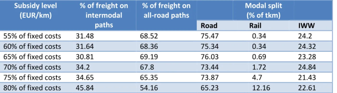
Based on previously held discussions with the involved actors in rail freight transport, a common affirmation was acknowledged about the necessity of rail subsidies for the survival of the business. In that respect and confirmed by the above negative results with respect to rail-borne flows, we use the same model SVN to test for the effects of rail subsidies on drawing flows to rail-based intermodal connections. We show in Table 6 different increasing figures of the considered subsidies and their impact on the resulting modal split, both for the reference- and medium-case scenarios. The levels of subsidies are represented in terms of fractions of the fixed costs of rail services.
Table 6: Impact of rail subsidies on the national flows’ repartition (Instance 1) (a) Reference scenario
Subsidy level (EUR/km) % of freight on intermodal paths % of freight on all-road paths Modal split (% of tkm)
Road Rail IWW
55% of fixed costs 31.48 68.52 75.47 0.34 24.2 60% of fixed costs 31.64 68.36 75.34 0.34 24.32 65% of fixed costs 30.81 69.19 76.03 0.69 23.28 70% of fixed costs 34.2 67.8 73.44 1.72 24.84 75% of fixed costs 34.65 65.35 73.87 4.7 21.43 80% of fixed costs 45.84 54.16 65.23 12.16 22.61 SOURCE:OWN COMPOSITION (b) Medium-case scenario Subsidy level (EUR/km) % of freight on intermodal paths % of freight on all-road paths Modal split (% of tkm)
Road Rail IWW
50% of fixed costs 32.41 67.59 74.86 0.33 24.81 55% of fixed costs 32.56 67.44 74.71 0.33 24.96 60% of fixed costs 33.93 66.07 73.33 0.66 26.01 65% of fixed costs 33.28 66.72 74.25 0.67 25.08 70% of fixed costs 40.72 59.28 68.12 2.85 29.04 75% of fixed costs 51.23 48.77 60.83 8.63 30.54 80% of fixed costs 59.48 40.52 54.01 15.87 30.12 SOURCE:OWN COMPOSITION
The first recorded subsidies’ levels represent the first levels after which rail services start receiving freight flows and the fixed costs of their running become justified. Given the considered costs’ framework, we observe through the above results that, for both scenarios, the increase in the rail flows is quite slow during the first levels of subsidies, up until a certain threshold (70% of the fixed costs, nearly 0.9 EUR/container) then the change undergoes fast leaps. This threshold could also be seen as rendering the rail fixed costs to become around eight times as much as the road fixed costs, thus closing the gap and reducing the rail costs from their original level: around fourteen times as much as the road costs. This result suggests that it is crucial to identify this nontrivial level for
each costs’ scenario through scientific means in order to be able to make educated decisions in what concerns the business’ sustainability and avoiding unnecessary capital spending. Additionally, it is noticeable that with increasing subsidy levels, IWW services start losing small fractions of their flows to rail in the reference scenario, as opposed to their steady flows in the medium case. Given the fact, that both rail- and IWW-based transport paths have quite similar pre- and post-haulage distances, we can eliminate the road taxes factor from our interpretation. This would leave us with the factor related to increasing the shipping demands from the reference to the medium-case scenario; the relatively higher payload of IWW-borne services could then partially explain their persistence to receive freight flows even when coupled with increasing rail subsidies.
3.2.
Generalized costs – RailNetEurope corridors:
Using the model SVN-GC, the costs’ scope is generalized to account for service quality aspects, basically, transit times, which will potentially become pronounced on longer corridors. For this experiment, we use the input data from instance 2, instance 3 and instance 4, comprising 137, 85 and 176 commodities (alternatively, shipping demands) respectively. Similar to the previous experiment, all-road paths are enabled for each O-D pair and the changes between the reference and medium-case scenario elements are tested (Table 7).
Table 7: Comparison between the reference and medium-case scenario within a generalized costs’ analysis (a) Instance 2 Scenario % of freight on intermodal paths % of freight on all-road paths Modal split (% of tkm)
Road Rail IWW
Reference 0.49 99.51 99.75 0 0.25 Medium-case 0.9 99.1 99.38 0 0.62 SOURCE:OWN COMPOSITION (b) Instance 3 Scenario % of freight on intermodal paths % of freight on all-road paths Modal split (% of tkm)
Road Rail IWW
Reference 3.64 96.35 97.39 0 2.61 Medium-case 3.43 96.57 97.5 0 2.5 SOURCE:OWN COMPOSITION (c) Instance 4 Scenario % of freight on intermodal paths % of freight on all-road paths Modal split (% of tkm)
Road Rail IWW
Reference 0.89 99.11 99.27 0 0.73
Medium-case 1.63 98.37 98.94 0 1.06
SOURCE:OWN COMPOSITION
As observed with the national flows, rail transport continues not to receive freight flows in these experiments as well as at the European corridors’ level. If anything, this further confirms the
previously drawn conclusion about the indispensability of offering rail subsidies to sustain the services in comparison with the more affordable road services. Even though the results show that the IWW services are generally receiving less freight flows than in the case with shorter connections, considering the overall larger shipping demands at the continental level, IWWs are receiving considerable flows in terms of tkm. Nevertheless, their relatively now weaker position with respect to all-road transport could be attributed on one hand to the increased fixed costs of IWW services over longer distance, and on the other to the additional constraints regarding resource balancing by imposing a return service on each offered long haul service. Finally, the increased weight on service quality, represented in transit times, is clearly a current disadvantage for intermodality with the considered high line delays for IWWs and the additional transhipment times.
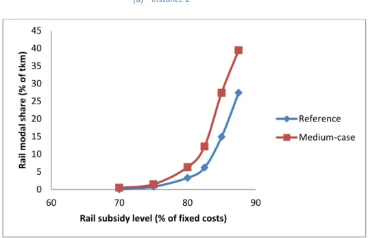
Now, we proceed by testing the impact of rail subsidies on the modal split at the continental level and how it could differ between the scenarios and with respect to the drawn conclusions in the previous domestic case as shown in Figure 2.
Figure 2: Impact of the rail subsidies on the flows repartition at the European level (a) Instance 2 SOURCE:OWN COMPOSITION 0 5 10 15 20 25 30 35 40 45 60 70 80 90 R ai l m o d al sh ar e ( % o f tk m )
Rail subsidy level (% of fixed costs)
Reference Medium-case
(b) Instance 3
SOURCE:OWN COMPOSITION
(c) Instance 4
SOURCE:OWN COMPOSITION
As it was previously observed, rail subsidies are necessary up until a certain threshold to sustain the services, after which more rail services can be offered, however at the expense of losing profits. The identified threshold in these sets of experiments is consistent with our previous findings at the domestic level: nearly 70% of the rail fixed costs. The starting level of subsidies differs according to the particulars of each corridor: principally the volumes of the shipping demands and how distributed they are along the corridor. Finally, it is shown that the medium-case scenario slightly dominates the reference scenario in terms of rail modal shares at each considered subsidy level. This remark suggests a decreasing need for supporting rail costs in a future plausible scenario, where road taxes are increased and there is more potential for consolidation with the growing freight demands. 0 5 10 15 20 25 30 35 20 40 60 80 100 R ai l m o d al sh ar e ( % o f tk m )
Rail subsidy level (% of fixed costs)
Reference Medium-case 0 5 10 15 20 25 30 35 40 45 60 70 80 90 R ai l m o d al sh ar e ( % o f tk m )
Rail subsidy level (% of fixed costs)
Reference Medium-case
4. CONCLUSIONS
In the context of testing the impact of certain instrumental changes on the intermodal freight transport and drawing insights about its potential future, we model a medium-term planning problem from the perspective of a freight transport services provider. For each shipping demand, there is the possibility of offering a direct all-road or intermodal service, where the latter, in addition to the pre- and post-haulage services, can be composed of rail, IWW services or a combination thereof. As a mathematical framework, we consider a service network design model to minimize the operating costs, where the decisions are mainly two-fold: the frequency of the transport services and the demands’ routing in form of itineraries. This model is later extended to account for service quality aspects: principally transit times, based on calculated weighting parameters through a discrete choice approach.
Two sets of experiments have been conducted, both at the domestic and the continental level. We summarize the most notable conclusions in the following points:
In the future medium case scenario, the increased road taxes have a significant
effect on drawing more flows to intermodal transport.
From a costs perspective, intermodal transport is more expensive to offer than
all-road transport, with a clear favouring of IWW over rail transport, potentially attributed to the high rail fixed costs. This observation holds at both the domestic (<300 km) and continental level.
IWW claim a weaker position on long corridors with respect to all-road transport,
potentially attributed to the additional costs related to the resources’ balancing and the difficulty to achieve high service quality reflected in long transit times.
Subsidizing rail services is necessary to make up for the high fixed costs. Experiments
have shown that most cases share a certain recommended figure for the required subsidies, in order to reasonably increase the rail modal share, after which the modal split undergoes fast unnecessary changes.
By comparing the two sets of experiments, we observe that intermodal transport
receive less modal shares on longer corridors across Europe, where additional resources balancing constraints are imposed and the service quality, represented in transit times, is optimized alongside the out-of-pockets costs.
As shown by the majority of experiments, in a future middle scenario, rail transport
REFERENCES
Andersen, J., Crainic, T.G., Christiansen, M. (2009). Service network design with asset management: Formulations and comparative analyses. Transportation Research Part C: Emerging Technologies 17(2) 197–207.
Agora, intermodal terminals database. http://www.intermodal-terminals.eu/
Bierlaire, M. (2003). BIOGEME: A free package for the estimation of discrete choice models.
Proceedings of the 3rd Swiss Transportation Research Conference, Ascona, Switzerland.
Carreira, J., Bruno, S. and Limbourg, S. (2012). Inland intermodal freight transport modelling. ETC Proceedings.
CE Delft, INFRAS, Alenium and HERRY Consult, External and infrastructure costs of freight transport Paris-Amsterdam corridor - Deliverable 1 – Overview of costs, taxes and charges, CE Delft, Delft 2010.
Crainic, T.G., 2000. Service network design in freight transportation. European Journal of Operational Research 122, pp. 272-288.
Crainic, T.G. and Kim, K.H. (2007) Intermodal transportation. Transportation Handbooks in Operations Research and Management Science. Chapter 8.
Emisia (2015). COPERT data for Belgium. Retrieved from http://emisia.com/products/copert-data .
European Commission, 2011. Transport White Paper: roadmap to a single European transport area – towards a competitive and resource efficient transport system.
European Commission, 2014. Scandinavian-Mediterranean Core Network Corridor Study. Final
Report.
http://ec.europa.eu/transport/themes/infrastructure/ten-t-guidelines/corridors/corridor-studies_en
Macharis, C., Janssens, G. K., Jourquin, B., Pekin, E., Caris, A. and Crepin, T. (2009). Decision support system for intermodal transport policy (DSSITP). Science for a sustainable development (SSD).
Newton, S. (2009). Deliverable 7. Freight Flows final. Worldnet Project (Worldnet.Worldwide Cargo Flows) Deliverable 7. Funded by the European Community under the Scientific Support to Policies
(Framework 6). http://www.worldnetproject. eu/documents/Public D, 7.
RailNetEurope. http://www.rne.eu/.
Vieira, L. F. M. (1992). The value of service in freight transportation. Ph.D. thesis, Massachusetts Institute of Technology.