Haeck: Department of Economics, Université du Québec à Montréal; and CIRPÉE Lefebvre: Department of Economics, Université du Québec à Montréal; and CIRPÉE lefebvre.pierre@uqam.ca
Merrigan: Department of Economics, Université du Québec à Montréal; and CIRPÉE
The analysis is based on Statistics Canada’s Survey of Household Spending (SHS) restricted-access Micro Data Files, which contain anonymous data. This research was funded by the Fonds québécois de la recherche sur la société et la culture. We are very grateful to Pierre-André Chiappori for his insight on lack of commitment Cahier de recherche/Working Paper 14-15
The Power of the Purse : New Evidence on the Distribution of Income
and Expenditures within the Family from a Canadian Experiment
Catherine Haeck Pierre Lefebvre Philip Merrigan
Abstract:
To increase mother’s participation in the labour market and enhance child development, the Canadian province of Québec developed from 1997 a large scale low-fee childcare network. Previous studies have shown that the policy has significantly increased the labour force participation and annual weeks worked of mothers with children exposed to the program. Using Statistics Canada’s annual 1997 to 2009 Survey on Households Spending we document the increase in the maternal share of total household income in Québec and use of instrumental variables approach to estimate the impact of the policy on intra-household expenditures. The results show that more income in the hands of mothers impacts the expenditures structure within the household by raising budget shares on expenditures related to children, family goods and services having a collective aspect.
Keywords: Childcare policy, mother’s labor supply, intrahousehold expenditures,
treatment effects, natural experiment
1
Introduction
For the last three decades, economic research on household choices has focused on explicitly modelling intra-household allocation within a bargaining framework adopting the ‘collective’ approach whereby household members each have their own preferences and reach agreements (or bargain) on a sharing rule that de…nes monetary transfers between members of the household. Hence, each member chooses his or her consumption and leisure subject to their own budget constraint partly de…ned by the sharing rule (Chiappori, 1988, 1992 for this landmark modelling). In general, group behaviour depends not only on individual preferences and the budget constraint but also on household members’respective ‘bargaining power’in the decision process. Any variable1that changes the bargaining power of household members
may have an impact on observed household behaviour.
Numerous empirical studies in developed and developing countries show that household members do not pool income (contrarily to the ‘unitary’ representation of the household characterized as common preference models). They also show that the share of income held by each spouse, when total income or expenditures is held constant, impacts household de-cisions and the intra-household allocation process. However, Lundberg, Pollak and Wales (1997) argue that earnings are endogenous with respect to the household’s allocation deci-sions implying that an instrumental variable approach should be used when estimating the impact of, for example, the share of female income in the household on the allocation of resources within the family.
This paper contributes to the empirical literature on the in‡uence of women’s bargain-ing power on household expenditure patterns. We use a policy experiment in Québec, the second most populated province in Canada, that considerably lowered the price of childcare for young children, to identify the impact of the share of female income in the household on a large array of consumption shares for households with children. Using Statistics Canada’s annual Survey of Household Spending (SHS) spanning the years 1997 to 2009, we demon-strates that this important daycare changed the share of income within the household in families with young children in favour of mothers. Then, using the policy as an instrument, we estimate by GMM the impact of the mother’s share of income on expenditure shares for categories of goods and services that are related to children’s well-being and development (for example health, education expenditures). The results provide evidence on the in‡uence of a universal childcare policy on expenditure shares related to children and the collective functioning of the family by way of a change in the bargaining power of mothers. Falsi…ca-tion exercises produced with couples without children as well as couples with older children not a¤ected by the policy provides further evidence enhancing the validity of our approach.
The remainder of the paper is as follows. Section 2 presents the low-fee childcare policy, childcare use and arrangements from 1997 to 2012 and traces the unique evolution of Québec among Canadian provinces. Section 3 brie‡y reviews the main principles and results from collective household models. Section 4 lays out the estimation strategy. Section 5 describes the data set, samples, and variables used in the analysis. It also describes the stylized facts on income shares within the household and the labor supply of mothers and fathers from 1997 to 2009. Sections 6 and 7 present respectively the main results and some falsi…cation exercises. Section 8 concludes.
2
Québec’s childcare policy
On September 1st 1997, all licensed and regulated childcare facilities (not-for-pro…t centres,
family-based daycare and for-pro…t centres) under agreement with Québec’s Ministry of the Family and Elders started to o¤er spaces at the reduced contribution of $5 per day per child, for children aged 4 on September 30th. On September 1st 1998 and on September 1st
1999 respectively, the 3-year-olds and 2-year-olds (on September 30th) became eligible for
low-fee spaces. On September 1st 2000, all children aged less than 5 years of age (if not age
eligible for kindergarten) became eligible for low-fee spaces.2 The government progressively
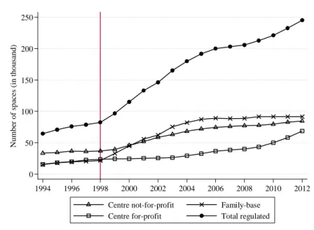
increased the number of subsidized $5/day childcare spaces from then on. The total number of partly subsidized spaces in the network increased from 78,864 in 1997 to 133,250 in 2001 when all children under 5 became eligible. In 1997, none of the spaces were at the low fee of $5/day, while most regulated spaces became “low-fee” by 2001. By March 2012, the number of regulated spaces reached 245,107 (with 89% "low-fee"). This represents a 211 percent increase over the 1997-2012 period.3 Figure 1 shows the evolution of the number of
regulated spaces from 1994 to 2012.4
Because the number of spaces increased over time and the entry age decreased between 1997 and 2000, not only did the number of children bene…ting from low-fee childcare in-creased, but also did the average number of years children spent in low-fee childcare or any type of care outside the home. In 2000, 39% of all children aged 1 to 4 were in low-fee
2For children aged 5 on September 30th1997, full-day instead of part-day kindergarten was o¤ered by all
School Boards across the province. Kindergarten is not compulsory but if a child is enrolled in a public school, he or she must attend class for the full school day and school week. All provinces o¤er publicly provided free kindergarten for 5-year-olds in a school setting under the auspices of the Ministry of Education. New-Brunswick, Nova-Scotia, and Québec (since the fall of 1997), o¤er full-time kindergartent, while in other provinces kindergarten is o¤ered half-day (2 hours and 30 minutes)during the period of our study. Haeck et al. (2013) show that the kindergarten policy by itself did not have an impact on the labor force participation of mothers, but the combination of the low-fee daycare program and full-day kindergarten did.
3All statistics are from Haeck et al. (2013) who present additional information on the childcare policy.. 4Information on the number of low-fee spaces is only available as of 2001. As such, it is not possible to
childcare services, 47% in 2002, 56% in 2004, 61% in 2006, and 59% in 2009.5 Haeck et al. (2013) also show that the participation rate in child care increases with the age of the child and that the number of hours spent in childcare conditional on attending childcare also increased over the period. This may be attributed to the long opening hours of the low-fee childcare centers. In the Rest of Canada (RofC, hereafter for the other provinces) there was no such major change in the childcare policy (Haeck et al. 2013).
The policy pursued two major objectives: to increase mothers’ participation in the la-bor market and to enhance child development and equality of opportunity. Studies on the Québec childcare reform show that it had a signi…cant positive impact on the labor supply of the mothers of eligible children in Québec. Lefebvre and Merrigan (2008) use annual data from 1993 to 2002, drawn from Statistics Canada’s Survey of Labour and Income Dynamics (SLID), with a sample of Canadian mothers with at least a child aged 1 to 5, and estimate a substantial e¤ect of the policy on a diversity of labor supply indicators (participation, labour earnings, annual weeks and hours worked). In 2002, the e¤ects of the policy on participation, earnings, annual hours and weeks worked of the childcare policy are estimated to be respec-tively between 8.1 and 12 percentage points, $5,000-$6,000 (2001 dollars), 231 to 270 annual hours at work, and 5 to 6 annual weeks at work. Baker et al. (2008) using the …rst two cycles (1994-1995 and 1996-1997) and the last two cycles (2000-2001 and 2002-2003) then available of the National Longitudinal Survey on Children and Youth (NLSCY), also provide evidence of a substantial e¤ect of the policy on mothers’employment and non-parental childcare use. Finally, Lefebvre, Merrigan, and Verstraete (2009), with annual data from the SLID (1996 to 2004), using a triple di¤erence approach …nd that the program had substantial dynamic labour supply e¤ects on mothers in Québec, in particular for cohorts of mothers who had a high probability of receiving subsidies from the child’s birth to his or her …fth birthday.
Therefore, since 2000, labor supply and earnings of mothers with children 0 to 11 have substantially increased in Québec relative to the RofC. We show below that this translated into an increase in the share of female income in the household in Québec relative to the RofC. This exogenous variation allows us to estimate the impact of the share of female income on consumption shares in the household.
3
Collective household behaviour
Many public policies, in developed and developing countries, use targeted bene…ts to par-ticular members in families to promote speci…c outcomes, in parpar-ticular for children. Many studies in the last decade have shown that investing in young children may be the best
5Families who do not have a low-fee space can use ‘private’ childcare and bene…t from the Québec’s
strategy to enhance their well-being and skills (cognitive, social, behavioral, health) while reducing disparities among young adults (Cunha and Heckman, 2010; Almond and Currie, 2011).
A common assertion is that ‘mothers care more for children than fathers’, thus allocating more expenditures and parental time for them. This statement should be soundly analysed to shed light in types of public policies that may most successfully bene…t families and children. Lundberg and Pollak (1996) resume in a biting way the thinking in the mid 90s:
“The most provocative within this brand of empirical work demonstrates a strong positive association between child well-being and the mother’s relative control over family resources and has raised new questions about the potential e¤ective-ness of policies ‘targeted’ at speci…c family members. . . However, no new theo-retical framework has gained general acceptance as a replacement for common preference models, and empirical studies have concentrated on debunking old models rather than on discriminating among new ones.” (p.140)
The …rst assertion has been illustrated in numerous empirical studies, pointing to the fact that each spouse has a di¤erent impact on household decision making. Among the most cited studies, Lundberg, Pollak, Wales (1997) exploit the change in the UK child support system which resulted in bene…ts being paid to the mother instead of the father (a shift ‘from the wallet to the purse’). They show that this policy lead to signi…cant increases in the share of expenditures for children’s clothing and women’s clothing over expenditures for men’s clothing.6 Bourguignon, Browning, Chiappori, and Lechene (1993, 1994), using
French and Canadian data on consumer spending, as well as Phipps and Burton (1998) with Canadian data, show for spouses working full-time without children that relative spouses’ income has a signi…cant impact on intra-household expenditures.
In developing countries, Thomas (1990), Schultz (1990), Hodddinot and Haddad (1995) for example, present empirical evidence that income and the female’s share of non-labour income within a couple (women’s share of cash income, or wealth at marriage) have a signif-icant impact on children’s health, fertility or food shares, as well as alcohol and cigarettes consumption (Brazil, Indonesia, Côte d’Ivoire). Du‡o (2003) obtains a similar qualitative e¤ect when analysing the reform of the South African social pension program, which ex-tended bene…ts to a large black population (in particular grand-mothers). This windfall generated improvements in child nutrition which depended on the gender of the recipient. Similar …ndings are found in the Mexican ‘Progresa (Oportunidades) program’(and its other Latin America counter parts), a subsidy program that provides educational grants to the
6Ward-Batts (2008) uses the same quasi-experiment to provide evidence that demand for male tobacco
poorest families in rural Mexico if mothers insure their children go to health clinics and attend schools (Behrman et al. 2011; Behrman 1997). Such …ndings have potentially crucial normative implications on the design of aid policies, social bene…ts, taxes, and other aspects of public policy.
The second assertion on modelling no longer holds: since the collective barganing ap-proach has become a mainstay in labor economics (see Chiappori and Donni, 2010). The main elements of the basic structural model (a two-member household where both work and consume only private market commodities and leisure, and have speci…c preferences; and only observable are household total consumption, individual wages and non-labour income) are the following. The only assumption is that intra-household decisions are Pareto-e¢ cient bargaining between members: there does not exist a bundles of consumption and leisure which can increase the welfare of the members. In this type of model, preferences are de-pendent on wages, prices, and individual non-labour incomes all assumed exogenous. Thus, the household maximize its welfare taking into account the individual utility subject to the household budget constraint.7 The utility of each member has a welfare weight, which can be interpreted as the bargaining power of household members. This sharing rule (which speci…es the allocation of income between members) can be identi…ed up to an additive con-stant as well as the underlying individual preference parameters (up to a transformation). In this context, the bargaining power of members will depends on prices, wages and non-labour income. Thus source of non-labour income may be important for the household allocation and may be impacted by public policies, such as targeted transfer bene…ts.
Critical and relevant to this paper, Mazzocco (2007) explains that in a life-cycle set-ting with commitment between members of the household, no policy will be e¤ective in changing bargaining power within the household, but the contrary is true in the absence of commitment. Estimate of a life-cycle collective model strongly rejects commitment, thereby rendering feasible policies that seek to a¤ect bargaining power within the household. In line with Mazzocco, we suppose that the cross-sectional families of the SHS surveys are charac-terized by lack of commitment. Browning, Chiappori, and Weiss (2011) discuss extensively the importance of commitments (how much to invest in children, how much to consume each period, proportion of family assets that each partner would receive upon divorce) made at the time of marriage to attain e¢ cient investment and consumption outcomes. They also ar-gue (p. 270) that Mazzocco …ndings indicate that cross-sectional and longitudinal variations in relative decision power explain a part of the sensitivity of consumption to income shocks.
7Technically, given the assumptions of e¢ ciency and egoistic or caring preferences, the household decision
process can be reduced to a two-stage decision process. In the …rst stage, non-labour income is shared among household members according to a sharing rule. In a second stage, each individual separately allocates his or her income to its own consumption and leisure in a way that maximizes his or her own utility subject to an individual budget constraint.
Though, such variations are important to understanding the dynamics of household con-sumption and policy changes. Another implication is that the principle on non separability between consumption and leisure may not longer strictly apply.
The childcare universal policy is an exogenous variation impacting the labor supply of mothers (not fathers) and therfore the income share of mothers within the household. The policy. acts as a ‘distribution factor’providing more power to mothers over household allo-cations and to express their di¤erences in preferences).
4
Empirical estimation strategy
A non-experimental evaluation framework based on multiple pre-and post-treatment periods is used to estimate the policy e¤ects on the share of female income in the household in the …rst step of our two-stage strategy.
Formally, the …rst-stage regression instruments the endogenous variable, the share of the mother’s total income in both spouses’ total income. The equation for the …rst step is as follows: M_Shareit = + 1QCit+ 2P ostit+ 2009 X t=2001 tQCit Dit+ 0 Xit+ "it; (1)
where M _Shareit represents the mother’s income share for family i in year t. The term
QCit takes the value of 1 if family i lives in Québec in year t, and otherwise takes the value
0. P ostit is a dummy variable indicating the post-treatment period for the main sample,
representing the e¤ect of a post-policy aggregate e¤ect common to both regions. The terms
t represent the e¤ects of the policy over time as the QCit dummy is interacted with year
dummies, Dit (t = 2000; :::; 2009). These post-policy period interaction dummies are the
instruments of the model. The e¤ect of the reform is di¤erentiated over time as additional subsidized spaces were added to the daycare network in Québec over this period. The term Xitis a vector of socioeconomic control variables and is a vector of parameters. Finally, "it
is an i.i.d. error term.
The decision on pre-reform and post-reform periods as well as the age groups of children potentially eligible to low-fee childcare determinates the choice of instrumental variables (post-policy interaction dummies).8 As of September 1997, the only bene…ciaries of the
policy were families with a 4-year-old child already in child cared in the regulated network. As such, it is unlikely, however, that the policy impacted families’ labor force behavior or expenditures at the dawn of its implementation (Haeck et al. 2013 for evidence). Each
8In the early years of the program, already available spaces were converted to $5/day spaces but no new
September after 1997 until September 2000, the age eligibility for low-fee childcare widened from age 4 to ages 0-1 in 2000. However, very few new subsidized childcare spaces were created in 1998 and 1999, although private providers joined the regulated network and thus began asking $5/day for children already in childcare. The addition of new low-fee spaces really took o¤ in the mid-1999 (spaces are created every month) and large yearly increases persisted until 2006. Thereafter, new spaces were added at a much lower rate. Since the SHS reports yearly expenditures, our pre-reform period end in 2000.
The second stage estimation …ts expenditure shares on the instrumented M _Shareit and
exogenous variables.
C_Sharekit = 1+ 2M\_Shareit+ 3QCit+ 4P ostit+
0
Xit+ uit; (2)
where C_Sharekit represents the share of expenditures for good k in family i in year t.
As for socioeconomic control variables, we retained the mother’s age and age squared, the number of children aged 0-4, 5-14, and 15-19 years, the total number of children in the household, seven categories for the size of the area of residence, total real family consumption, a common linear trend, as well as provincial dummy variables.
5
Data and variables
Data and samples Our data are extracted from Statistics Canada’s SHS for the years 1997 to 2009, a yearly survey with a cross-sectional design collecting detailed information on household annual expenditures.9 The survey contains detailed information on expenditures
for consumer goods and services. Annual samples of approximately 15,000 households (except for the 2008 and 2009 surveys which provide approximately 10,000 households) also provide information on the annual income of household members (extracted from individual tax retourns, in a majority of cases), on some demographic characteristics of the household, on dwellings (e.g., type, age and tenure) and household equipment (e.g., car, appliances, electronics and communications equipment).10 Because the SHS is designed principally to
9The target population is the population of Canada’s 10 provinces, excluding residents of institutions (e.g.
prisons, hospitals) members of the Canadian Forces living in military camps and people living on Indian reserves. In all, these exclusions make up about 2% of the population of the 10 provinces. Conducted since 1997, the Survey of Household Spending integrates most of the content found in the Family Expenditure Survey (FAMEX) and the Household Facilities and Equipment Survey. The preceding survey, FAMEX, was conducted every four years; the last one was conducted in 2006.
10De…nitions of the majority of variables used in this study remained unchanged over the years 1997-2009.
See Statistics Canada (http://www.statcan.gc.ca/pub/62f0026m/2012002/change-eng.htm#a6) for changes since year 2010. The SHS combines two collection methods (recall periods based on the type of expenditures and a daily expenditure diary that the household completes during a two-week period following the interview). The master …le of the 2010 SHS was not available at the time of this research.
provide detailed information on non-food expenditures, only an overall estimate of food expenditures is recorded in the survey as well as expenses for food purchased from stores and food consumed outside the home which are recorded separately.
For the purpose of this study, our main sample is restricted to households, were both spouses are present and who have at least one child less than 15, and with the female spouse aged 20 to 51.11 For fathers, the age restrictions are from 20 to 60 to exclude students and pensioners. The selection leaves us with 5,160 couples with at least one child aged 0 to 14 in Québec and 33,489 similar couples in the RofC for the period of 1997 to 2009.
Dependent and explanatory variables The SHS groups expenditures for individual items into a large number of categories which are then further aggregated into 14 broad groups of goods and services: expenses incurred during the survey year for food (in stores, and in restaurants or take-out settings), shelter, household operations, household furnishings and equipment, clothing, transportation, health care, education, personal care, recreation and leisure goods and services, reading materials, tobacco products and alcoholic beverages, games of chance, and a miscellaneous group of items. The sum of these 14 categories is considered as total current consumption (that is excluding personal taxes, personal insurance payments and pension contributions, and gifts of money and contributions to persons outside the household). The de…nition of the categories are presented in Table A.??
For some of these categories we changed some of the items included First, we deleted from some categories, items that can be considered as durables, infrequent or very selected expenditures: we kept shelter expenditures for the principal residence (usual expenditures in-cluding public services, exin-cluding expenses for traveller accommodation and vacation homes); for transportation, we used direct expenditures for private and public transportation (ex-cluding purchases or sales of vehicles); for the recreation category we also excluded purchases or sales or operation of durables such as recreational vehicles. We also retained a few more narrow groups of expenditures. The large clothing category can be examined for three groups by speci…c gender and age of household members: total clothing expenses for children less than 5, for women and girls aged 5 or more, for men and boys aged 5 or more. From the recreation items, we constructed a leisure goods and services category more speci…c to chil-dren (although parents may also likely consume such goods): sports equipment, toys, games and hobby material, bicycles, video tapes, DVDs, video games (buy or rental), admission to movies, live-arts heritage facilities, and children’s camps. Second, we de‡ated total current consumption and the 14 expenditure categories by province speci…c price indexes ($2001) constructed by Statistics Canada. Third, we computed expenditure shares (expenses in a
11To minimizes the number of spouses who may be a studeunt. Throughout the term spouse refers to
category of spending to total current consumption, the latter de…ned by the aggregation of all categories) for each household.
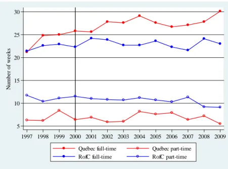
Like many other household traditional expenditure surveys, the SHS does not contain information on the speci…c expenditures made by di¤erent members of the household (except clothing by sex). There are no information available on wage rates, hours or work, and no assignable commodities for members of the household, but only spouses income and house-hold expenditures (some with a private component and other with collective characteristics) are available. Also, the SHS has limited information on household sources of income and labour market activities. Four variables measure the annual income of each spouse and of the household, they are: 1. total income from earnings (paid work, net income from self-employment, and income from roomers and boarders); 2. total income from investments; 3. total income from transfer payments by the governments; 4. and, total income from other sources. Only three labor supply measures are available: number of weeks worked full-time and part-time by each spouse, and employment status during the survey year (grouped into three categories working full-time, part-time, and not working).12 Thus, hours of work and hourly wages are not derivable from the information included in the data set. Our measure of the bargaining power within the household (‘distribution factor’) is de…ned by the ratio of the mother’s income over total income accruing to the two spouses.13 The other spousal preference markers are demographic characteristics of the household which we use as control variables: age of the spouses, the population area size in which the household resides; the exact number of children by age group (0-4, 5-14, 15-19), and the age of the youngest child.14 Descriptive statistics and stylized facts on labour supply Figure 2 and Table A.1 (columns 1 and 3 to 5) display three important features of annual weeks worked. First, a large proportion of mothers do not work (column 5); when they do, however, the range of weeks that they supply over time is rather large (column 1).15
Second, it is well known from other surveys (e.g. Labour Force Survey) that working mothers with young children in Québec prefer a full-time job compared to similar mothers in the RofC (from columns 1 and 3). Patterns of full-time and part-time weeks worked shown
12Full-time if weeks worked full-time plus part-time weeks>= 49 and full-time weeks >= 25; part-time: if
weeks worked full-time plus part-time weeks = 1 to 48 weeks worked full-time weeks plus part-time weeks >= 49 and full-time weeks < 25; did not work if full-time weeks plus part-time weeks = 0. Maximum value of weeks worked is 52.
13Since the selected households all have rather young children, the gap between household total income
and total income of both spouses is small.
14Beginning with year 2004, the age and sex of each child, the highest level of education attained by each
spouse as well as if a spouse has a disability are provided with the master …les, but these years are all in the post-reform period.
15For example, in year 1997, 47 percent of Québec’s mothers do not week, 30 percent work 52 weeks and
in Figure 2. The latter is rather ‡at for both regions. More importantly, the divergence in the evolution of labor supply between Québec and the RofC can be observed for full-time weeks beginning in 1998 (…rst full year of the low-fee policy for the 3 to 4-year-olds with no new childcare spaces). The gap increases over the years as the policy is fully implemented and new childcare spaces are added each year. In 2007 and 2008, the percentage of Québec mothers working 52 full-time weeks was respectively 40 and 45 percent compared to 36 and 33 percent for mothers in the RofC (Table A.1 column 1). In Québec, the evolution of mothers’ labor force status has as also changed considerably compared to mothers in the RofC (Table A.1 columns 3-5), in particular since year 2000: a larger percentage works full-time and a lesser percentage is not working; in the RofC, although a large proportion is attached to the labor market, the percentage not working has not changed over time. Years 2008 and 2009, however, show that the …nancial crisis may have impacted labor force behavior.
Third, most fathers work full-time, on average 45 weeks per year, with marginal variations over time except in 2009 (statistics not shown in Figure 2). Part-time work or not working Table A.1 (columns 1 and 6 to 8) are chosen by few fathers. There is no discernable trend over the years, except for a small drop in participation corresponding to the …nancial crisis in 2008 and 2009. As to the number of weeks worked (Table A.1), few fathers do not work full-time. The spread in weeks is much smaller than for mothers, and a large proportion works all 52 weeks of the year.
Figure 3 illustrates the potential impact of the childcare policy on the economic impor-tance of mothers for family expenditures. We show for both regions the average share of mothers’income and her average share of earnings over time for both regions. In Québec, there are large increases in mothers’total income shares after 2000, which can be linked to the raise in earnings due to the childcare policy. For the RofC mothers, the earnings’share is ‡at from 2001 to 2008. The exception is year 2009, where mothers seem to have coped with the …nancial crisis by working additional weeks as many fathers lost their jobs and were likely constrained in their number of full-time weeks worked (see Figure 2 and Table A.1). Clearly, the mothers’share of income has been a¤ected by the childcare policy.
Table A.2 displays descriptive statistics for the main sample (families with a youngest child aged 0 to 14) used for the estimation, by region.16 We observe that families on average are very similar in terms of the control variables that will appear in the regressions (age of the mother, of the father, household size, and the size of the area of residence). The main di¤erences are in the mean number of children in the two age groups, and evidently the mothers’share of income in family income.
Finally, we constructed similar statistics for women in a couple with no children at home, adopting the same selection criteria as in the main sample (except of course for the age of
children) (Table A 3). Statistics (Table A.3, columns 10 to 13) suggest that they have worked more full-time weeks, that their is a larger proportion working full-time in Québec than in the RofC. And the same trends are observed in both regions. The women in couples with no children in Québec and RofC (Table A.3), are also very similar in terms of demographic characteristics and work behaviour over the sample time period.
The expenditure share categories over the years 1997 to 2009 are presented for families with children by region in Table A.4. Six categories (food, main shelter, household operation, clothing, transport, and leisure) represent on average 80 percent of expenditures. The food share is larger in Québec and has signi…cantly decreased for both regions. The share for the main shelter is higher in Québec and has marginally decreased in both regions. For household operations and clothing shares, di¤erences and trends by year and region are more marginal. For transport and leisure, we notice large increases over time in both regions. The tobacco and alcohol, and lottery game shares, although small, have consistently decreased over time in both regions. The shares for couples with no children (not shown) indicate that they are almost all the same over regions and years.
6
Results
Above we indicated that the full childcare policy was implemented over 4 years (September 1997 to September 2000) and that new spaces were added only from year 1999. In the case of ineligible lower aged children, it is possible that parents were informed that low-fee caregivers would eventually provide a subsidized space when the child got older and rushed into the labour market after the birth of the child to be in a position to eventually obtain a subsidized space. The government also publicized (at the announcement of the policy in January 1997) the need to place a child in a subsidized daycare setting as early as possible. There was a very strong incentive to obtain a space early on to reap bene…ts from the policy for as many years as possible. This incentive was lower for mothers with children aged four or three in the …rst years of the policy as, in their case, the bene…ts of the new policy lasted for a much shorter time.
Furthermore, given the results in Lefebvre and Merrigan (2009) which show that the policy probably incited mothers that would not have returned in the labor market even when the child entered school in the counterfactual world of no daycare low-fee policy, to join the labour market when the child is very young and stay there for good or until she gives birth again, it is feasible that the policy could a¤ect relative income shares in families where children are no longer of daycare age. Henceforth, because age 4 children in 1997 (…rst group of children potentially but unlikely touched by the policy) are 16 years-old in 2009, we consider families with a 15 year-old child or younger in 2009 may have been a¤ected by the
policy. Children aged 3 or 4 in 1998 (second year of implementation) are aged 13 or 14 years in 2009. The 0 to 4 year-old children in 2000 are aged 9 to 13 in 2009. Therefore, as our base sample we selected couples with at least one child aged 0 to 14 years with the post-reform period chosen to be 2001. We also conducted estimations for families with children aged 0-15 and 2001 as the post-reform period to examine the sensibility of results with the chosen windows.
We conducted GMM estimations of equations (1) and (2). We also performed GMM es-timations using two alternative instrumental variables in lieu of post-policy period interacted dummies. The second set of instrumental variables are the post-policy yearly instruments interacted with a dummy if the youngest child in the household is eligible or had been eligible for subsidized daycare: at 4 in 1998, adding eligible children by the age of the youngest child each year till 2009 (3, 2, 1-0, and 5, 6,... to 14 or 15 years). Finally, we provide estima-tions with the number of regulated childcare spaces for children 0 to 5 years old and before-and after-school for kindergarten for a sample of families with at least one child 0 to 12 by province and for the years 1997 to 2009 as instrument.17 That is, the number of childcare spaces are divided by the number of children aged 0 to 12 years in each province.18
We performed three series of estimations, each with the three instruments. The …rst one with a sample of households with children 0 to 14 years of age. In the second series of estimations we changed the age groups of children (0 to 5, 0 to 10) more directly a¤ected by the policy. In a third series, as falsi…cation exercises we changed the sample years and the age groups of children to estimate the model with families from Québec that were not exposed to the childcare policy and their counterparts in the RofC. Samples based on the age groups of children that were not eligible for the policy were selected as placebo groups: children aged 11-17 from 1997-2000 (with post-reform period 2001-2009), and children aged 9-14 in 1997-2000 (with post-reform years 2001-2004) We also estimated the impact of the policy for couples with no child present in the household. Finally, we conducted statistical tests of under or weak identi…cation, excluded instruments, and over-identi…cation.
The GMM policy estimates ( 2M_Share\ itcoe¢ cients in equation (2)) results for the 17The data set is provided by Friendly et al. (2012). The number of regulated and subsidized spaces are
a policy decision since the creation of new spaces may imply public subsidies (to providers and to families depending on their income in the Rest of Canada). For Québec, the policy is a costly one. In 1996-1997, public subsidies amounted to 288 million dollars. Under the childcare reform, these subsidies were gradually abolished. Instead, the regulated and subsidized childcare providers receive a …xed amount per child per day, depending on the age and type of childcare setting, complemented with the low-fee contribution of the family. By 2011-2012, the total government subsidy reached 2.2 billion. In the …rst year of the policy (covering only the 4-year-olds and continuing parental fee-subsidies for the other children in daycare), the mean subsidy per space was $3,888. For …scal year 2011-2012, the mean subsidy amounted to $10,210 per space.
18For Québec, the ratio is 0.057 in 1997 and increased every year to 0.204 in 2009. In the Rest of Canada,
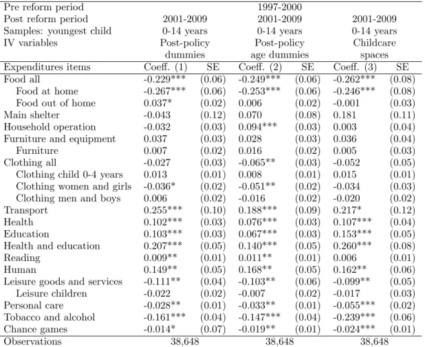
main sample (couples with children aged 0-14)19 are presented in Table 1. Results are presented with the three alternative IV’s. The three sets of instruments used are: (1) post-policy dummies, (2) post-post-policy age dummies, and (3) number of childcare spaces by year and province.
In all three cases, the mother’s share of income has a negative and signi…cant e¤ect on overall food expenditures. The e¤ect on food expenditures out of home is generaly possitive but not always signi…cantat home (food stores) and positive but not always signi…cant e¤ect for food out. This suggests a small substitution of food at home for food out (restaurants and take-away). Increased labor force participation of mothers implies that they are away away from home at lunch time (for example), and have less time to prepare food at home.20 The e¤ect on “main shelter” expenditure shares is not statistically signi…cant except when the number of childcare spaces is used as the instrument (column 6). The household operation share coe¢ cients are positive and signi…cant, but only with post-policy dummies interacted with age eligibility as instruments. No signi…cative positive e¤ects are found for furniture and equipment.
For the clothing categories (all types, for very young children, for women and girls, and for men and boys) coe¢ cients in almost all speci…cations are not statistically signi…cant, except in some cases for women and girls’(aged more than 4 years-old) clothes, with a signi…cant and negative e¤ect. One drawback of the data set is that we cannot distinguish adults’ clothing expenditures from childrens’. The increases in the mother’s income share may drive con‡icting changes in the di¤erent clothing categories. The coe¢ cient of the mother’s share on clothes for the 0-4 year-old children suggests a positive e¤ect but it is almost always not signi…cant.
Not surprisingly, the shares for transport increases signi…cantly, simply because more Québec’s mothers must travel to work and bring their younger children to childcare facili-ties.21
The e¤ect of the policy on the share of health expenditures, education and the aggregate of health and education are positive and signi…cant. The e¤ect is also generally positive and signi…cant for the share of reading materials. Under the aggregated category human, we have included household operation, education and reading expenditures. Theses are associated with child well-being and allow us to assess the overall impact of mothers income shares on goods and services that are collective in nature. We …nd a strong positive and signi…cant e¤ect. This suggests increased maternal income share of total household results
19The results for the 0-15 years are vey similar and available on request. 20These e¤ects may be linked to types of food consumed at home.
21The proportion of families (with at least a child aged 0-14 years with) in Québec with two cars has
increased from 33 percent for years 1997-2000 to 40 percent in 2009, while in the Rest of Canada the proportion has remain relatively constant, at approximately 41 percent.
in the family investing more in collective goods that likely bene…t children. These results corroborate previous evidence discussesd earlier.
The share of leisure commodities have negative and signi…cant coe¢ cients, except when it is more narrowly de…ned as leisure good and services more related to children, all non signi…cant. The results for share of total personal care indicate strong negative signi…cant e¤ects in all cases, which in not surprinsing considering that mothers (and fathers) have less time to spend for such activities for themselves for their children.
The last two categories, tobacco and alcohol, and games of chance (government-run lotteries, casinos, bingos, non-government lotteries, less game winnings in dollars) show negative coe¢ cients A.4). These results also support the idea that higher mothers’income shares may pressure against some adults goods.
These shares are of interest because they may be associated to certain members of the family: mothers, fathers, and children. Although, this empirical model cannot tell which members have bene…ted most, as well as the collective characteristics of these expenditures, the e¤ects suggest that mothers income’shares have played a role in intrafamily allocation. Québec’s families have increased the shares of these expenditures (Table A.4) but mothers may have less time to spend in leisure activities for themselves and with their children.
The 5 panels of Table 2 present the same type of estimations for samples of families where the youngest children are aged between 0-5 or 0-10 years. The e¤ects are very similar. For the estimations with post-policy age dummies (panel 1), the signi…cant coe¢ cients are smaller than in the preceding estimations; with signi…cant positive coe¢ cients for the furniture and equipment category, transport, health, and negative e¤ects for tobacco and alcohol, and chance games. In panel (3), we also present results when using childcare spaces as instruments the youngest are aged 0 to 5 directly a¤ected. The e¤ects match those in the …rst two panels, the exceptions being main shelter, transport and personal care, which can be anticipated given that mothers spend more time with very young children having less time for personal care. Panels 4 and 5 present results with the …rst two sets of instruments providing the the same signi…cant coe¢ cient, adding the shelter share, which indicates that age of children impacts expenditures.
In sum, the results presented in Table 1 and Table 2 highlight two main impacts of the childcare low-fee policy. First, the main consequential e¤ects of mothers larger share of family income are related to shares that have a time component, such as food, transport and leisure goods and services. Second, the categories whose ratios have increased (household operation, health, education) or decreases such as the two “vice”categories, have appreciable direct impacts on family and children well-being, may be more than expenses on furniture and equipment and main shelter.22
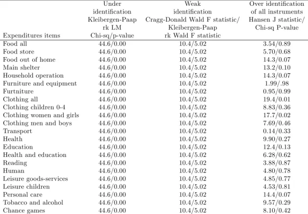
The statistical tests on instruments and identi…cation described in Baum et al. (2007) and Stock and Yogo (2005) are presented in Tables 5 and 6.23 Table 5 presents the coe¢ cients of the …rst two sets of excluded instruments (and childcare spaces as instrument). It is worth mentioning that the tests indicate that the coe¢ cients on the instruments in the reduced form equation for expenditure shares are statistically signi…cant (Angrist-Pische p-value of F test). Second, the most of the instruments are strongly signi…cant in the …rst stage. As for over-identi…cation tests (not presented), only once is the null rejected, what we expect from chance alone.
Table 6 presents tests for weak, under identi…cation for the …rst stage as well as the Hansen J statistic. We strongly reject the null that the model is underidenti…ed and do not reject the null that the instruments are uncorrelated with the second-stage error term. However, the model does suggest a problem of weak identifcation as the F statistic for the exclusion of instruments in the …rst stage is less than 10 and both the Craig-Donald Wald F statistic and Kleinberger Paap rk Wald statistic are rather small compared to critical values associated with small rejection rates.
7
Falsi…cation and placebo estimations
As a falsi…cation exercise, we re-estimated the expenditures share equations for families with children not exposed to the policy over the years considered.24
The …rst panel (1) of Table 3 present placebo results for families with no children present in the household, with post-policy dummies as instruments. The Québec women in these families are very similar to those in the RofC with respect to their demographic characteris-tics. We do not …nd signi…cant e¤ects except one or two as predicted by chance. The next four columns of Table 3 present results for families respectively, with children aged 11 to 17 years observed during the post reform period (2001-2009), and with children aged 9-14 years (period 2001-2005 as post-policy), with (1) post-policy dummies and (2) post-policy age dummies as intruments. Again, very few coe¢ cients are signi…cant (columns 2 and 3),.the last panels (columns 4 and 5) tell the same story.
declining cost of residence …nancing in the 2000s.
23We use the Stata ado program, ivreg2, developped by Baum et al. (2007).
24We also conducted the estimations excluding year 2009 from the post-reform period since the …nancial
shock and its impact of employment may have induced families to revise their expenditure patterns. The results without 2009 are vert similar.to those obtained with the full sample.
8
Conclusion
In this paper we estimate the e¤ect of the mother’s family income share on shares of ex-penditures in the household, for a given level of household exex-penditures, using public policy shocks arising from the development of universal low-fee childcare network in a large Cana-dian rovince, as instruments for the mother’s shares. Over the years, most of Québec’s mothers have reacted to the reform by increasing their labor force participation (at the extensive and intensive margins), and outpaced that of similar mothers in the RofC The policy augmented the share of mothers’ income within the household (earnings and total income), because fathers’ labor supply behaviour did not change compared to fathers in similar families in the RofC. This model is estimated for a sample of families in Québec and the RofC with children aged 0-14, and sub-samples of families di¤erentiated by type and the age groups of children. The impact of the mother’s shares on the ratios of expenditures for several goods are estimated using 3 sets of instrumental variables with GMM, to take into account the endogenous mothers’income shares.
The results show that for the sample of families covered by the reform, increasing moth-ers’share of income has a signi…cantly in‡uence on the structure of expenditures with more spending targeted to goods and services associated with children’s well-being and develop-ment. The e¤ects of mothers’empowerment (relative control over family resources) has been a di¢ cult challenge for collective labor model, considering empirically the paucity and limits of traditional surveys on expenditures (for use of a special data set, see Cherchye, De Rock, and Vermeulen, 2012). This paper suggests that a universal public policy (in this case child-care) may have long lasting in‡uence on children’s well-being by increasing the bargaining position of mothers.
9
References
1. Almond Douglas and Janet Currie (2011), “Human Capital Development before Age 5,”Orley Ashenfelter and David Card (eds.), Handbook of Labor Economics, Volume 4b, Elsevier, Chapter 5, 1315-1486.
2. Baker, Michael, Jonathan Gruber, and Kevin Milligan (2008), “Universal Child Care, Maternal Labor Supply, and Family Well-being,”Journal of Political Economy, 116(4):709– 745.
3. Behrman, Jere, Susan Parker, and Petra Todd (2011), “Do Conditional Cash Transfers for Schooling Generate Lasting Bene…ts? A Five-Year Follow-Up of Oportunidades Participants,” Journal of Human Resources, 46(1), 93-122.
4. Behrman, J. (1997), “Intrahousehold Distribution and the Family,” in Mark Rosen-zweig and Oded Stark eds., Handbook of Population and Family Economics, Amster-dam: North-Holland, Vol. 1A, 125-187.
5. Baum, C., M. Scha¤er, and S. Stillman (2007), “Enhanced routines for instrumental variables/generalized method of moments estimation and testing.”The Stata Journal, 7(1): 465-706.
6. Browning, M., P.-A. Chiappori, and Y., Weiss (2011), Family Economics. Cambridge University Press, forthcoming.
7. Bourguignon, F., M. Browning, P.-A. Chiappori, and V. Lechene (1993), “Intrahouse-hold allocation of consumption: a model and some evidence from French data,”Annales d’Économie et de Statistique, 29, 137-156.
8. Browning, M., P.-A. Chiappori, and Y„Weiss (2011), Family Economics. Cambridge University Press, forthcoming.
9. Browning M., F. Bourguignon, P. A. Chiappori, and V. Lechene (1994), “Children and Household Economic Behavior,” Journal of Political Economy, 1067-1096.
10. Cherchye, Laurens, Bram De Rock, and Frederic Vermeulen (2012), “Married with Children: A Collective Labor Supply Model with Detailed Time Use and Intrahouse-hold Expenditure Information,” American Economic Review, 102(7): 3377-3405. 11. Chiappori, P.A. (1988), “Rational Household Labor Supply,” Econometrica, 56(1):
63-89.
12. Chiappori, P.A. (1992), “Collective Labor Supply and Welfare,” Journal of Political Economy, 100, 437-467.
13. Chiappori, P.A. (1997), “Introducing Household Production in Collective Models of Labor Supply, Journal of Political Economy,” 105 (1): 191-209.
14. Chiappori, P.A. and O. Donni (2010), “Non-unitary models of household behavior: a survey of the literature,” in: A. Molina (ed.), Household Economic Behaviors, Berlin: Springer.
15. Chiappori, P.A, R. Blundell, and C. Meghir (2005), “Collective Labor Supply with Children, Journal of Political Economy,” 113(6): 1277-1306.
16. Cunha, Flavio and James Heckman (2010), “Investing in Our Young People,”in A. J. Reynolds, A. Rolnick, M. M. Englund, et J. Temple, eds., Cost-e¤ective Early Child-hood Programs in the First Decade: A Human Capital Integration, New York: Cam-bridge University Press, Chapter 18, 381-414.
17. Du‡o, E (2003), “Grandmothers and Granddaughters: Old Age Pension and Intra-household Allocation in South Africa,” World Bank Economic Review, 17(1): 1-25. 18. Friendly, Jane, Martha Beach, Carolyn Ferns, Nina Prabhu, and Barry Forer (2008),
“Early childhood education and care in Canada 2009,”The Childcare Resource and Re-search Unit, 8th edition, June, http://childcarecanada.org/publications; and "Trends and Analysis for 2010," 2013.
19. Haeck Catherine, Pierre Lefebvre, and Philip Merrigan (2013), “Canadian Evidence on Ten Years of Universal Preschool Policies: The Good and the Bad,”Working Paper 2013-17, CIRPÉE.
20. Hoddinott, John and Lawrence Haddad (1995), “Does Female Income Share In‡uence Household Expenditures? Evidence from Côte d’Ivoire,”Oxford Bulletin of Economics and Statistics, 57(1): 77-96.
21. Lefebvre, Pierre and Philip Merrigan (2008) “Childcare Policy and the Labor Supply of Mothers with Young Children: A Natural Experiment from Canada,” Journal of Labor Economics, 26(3): 519-548.
22. Lefebvre, Pierre, Philip Merrigan, and Matthieu Verstraete (2009) “Dynamic Labour Supply E¤ects of Childcare Subsidies: Evidence from a Canadian Natural Experiment on Universal Child Care,” Labour Economics, 16(5): 490-502.
23. Lundberg, S., R. Pollak, and T. Wales (1997), “Do husbands and wives pool their resources? Evidence from the U.K. child bene…t,”Journal of Human Resources, 32(3): 463-480.
24. Lundberg, S. and R. Pollak (1996), “Bargaining and Distribution in Marriage,”Journal of Economic Perspectives, 10(4): 139-158.
25. Mazzocco, Maurizio (2007), “Household Intertemporal Behaviour: A Collective Char-acterization and a test of Commitment,”Review of Economic Studies, 74(3): 857-895. 26. Phipps, Shelley and Peter Burton (1998), “What’s Mine is Yours? The In‡uence of Male and Female Incomes on Patterns of Household Expenditure,” Economica, 65 (November): 599–613.
27. Schultz, T. P. (1990), “Testing the Neoclassical Model of Family Labor Supply and Fertility,” Journal of Human Resources, 25, 4, 599-634.
28. Stock, J. and M. Yogo 92005), “Testing for weak instruments in linear IV regression,” in Identi…cation and Inference for Econometric Models: Essays in Honour of Thomas Rothenberg, ed. D. Andrews and J. Stock, Cambridge University Press, 80-108.
29. Thomas, D. (1990), “Intra-household resource allocation: an inferential approach,” Journal of Human Resources, 25(4): 635-664.
30. Ward-Batts, Jennifer (2008), “Out of the Wallet and into the Purse: Using Micro Data to Test Income Pooling,” Journal of Human Resources, 43(2): 325-351.
10
Figures
Figure 1: Number of regulated spaces
0 50 100 150 200 250 Numbe r of spa ces (in thou sand) 1994 1996 1998 2000 2002 2004 2006 2008 2010 2012
Centre not-for-profit Family-base
Centre for-profit Total regulated
Note: Shows the evolution of the number of spaces by mode of care between 1994 and 2012. As of 2001, all spaces are in
centre, not-for-pro…t, and family-based care. Most spaces in for-pro…t centre care are at the subsidized low fee. The number of
spaces is measured on March 31stof each year by the Direction générale des services de garde, Ministry of Families and Elders
(MFA). The vertical line marks the …rst post-reform year. The data can be accessed at www.mfa.gouv.qc.ca/fr/services-de-garde/portrait/places/Pages/index.aspx.
Figure 2: Average number of weeks mothers worked full-time and part-time by region
and year 5 10 15 20 25 30 N um be r of w e e ks 1997 1998 1999 2000 2001 2002 2003 2004 2005 2006 2007 2008 2009
Québec full-time Québec part-time
RofC full-time RofC part-time
Note: Shows the evolution of the average number of weeks worked full-time and part-time by region from 1997 to 2009. The
Figure 3: Average Mother’s share of total family Income by Region 24 26 28 30 32 34 36 38 40 Sh ar e i n p er c en tag e 1997 1998 1999 2000 2001 2002 2003 2004 2005 2006 2007 2008 2009
QC total income QC earnings
RofC total income RofC earnings
Note: Displays the avearge percentage of mother’s shares of family income by type and region between 1996 and 2009. The
11
Tables
Table 1: Impact of Québec’s mothers total household income share on selected intra-household expenditures shares
Pre reform period 1997-2000
Post reform period 2001-2009 2001-2009 2001-2009 Samples: youngest child 0-14 years 0-14 years 0-14 years
IV variables Post-policy Post-policy Childcare
dummies age dummies spaces
Expenditures items Coe¤. (1) SE Coe¤. (2) SE Coe¤. (3) SE Food all -0.229*** (0.06) -0.249*** (0.06) -0.262*** (0.08)
Food at home -0.267*** (0.06) -0.253*** (0.06) -0.246*** (0.08) Food out of home 0.037* (0.02) 0.006 (0.02) -0.001 (0.03) Main shelter -0.043 (0.12) 0.070 (0.08) 0.181 (0.11) Household operation -0.032 (0.03) 0.094*** (0.03) 0.003 (0.04) Furniture and equipment 0.037 (0.03) 0.028 (0.03) 0.036 (0.04)
Furniture 0.007 (0.02) 0.016 (0.02) 0.005 (0.03)
Clothing all -0.027 (0.03) -0.065** (0.03) -0.052 (0.05) Clothing child 0-4 years 0.013 (0.01) 0.008 (0.01) 0.015 (0.01) Clothing women and girls -0.036* (0.02) -0.051** (0.02) -0.034 (0.03) Clothing men and boys 0.006 (0.02) -0.016 (0.02) -0.020 (0.02) Transport 0.255*** (0.10) 0.188*** (0.09) 0.217* (0.12) Health 0.102*** (0.03) 0.076*** (0.03) 0.107*** (0.04) Education 0.103*** (0.03) 0.067*** (0.03) 0.153*** (0.05) Health and education 0.207*** (0.05) 0.140*** (0.05) 0.260*** (0.08)
Reading 0.009** (0.01) 0.011** (0.01) 0.006 (0.01)
Human 0.149** (0.05) 0.168** (0.05) 0.162** (0.06)
Leisure goods and services -0.111** (0.04) -0.103** (0.06) -0.099** (0.05) Leisure children -0.022 (0.02) -0.007 (0.02) -0.017 (0.03) Personal care -0.028** (0.01) -0.033** (0.01) -0.055*** (0.02) Tobacco and alcohol -0.161*** (0.04) -0.147*** (0.04) -0.239*** (0.06) Chance games -0.014* (0.07) -0.019** (0.01) -0.024*** (0.01)
Observations 38,648 38,648 38,648
Note: The dependent variables are expenditure shares. All speci…cations control for the real total consumption, age
and age squared of the mother, number of children by age group (0-4, 5-11, 12-19), size of the community (six groups from rural to 500,000 or more the omitted group), post policy indicator, linear time trend, year dummies (omitted 1997), provincial dummies (omitted Québec) SE: Standard error Coe¢ cient signi…cance is denoted using asterisks: *** is p<0.01, ** is p<0.05, and * is p<0.1 Human: household operation, education, and reading.
T a b le 2 : Im pa c t o f Q u é b e c ’s m o t h e r s t o t a l h o u se h o l d in c o m e sh a r e o n se l e c t e d in t r a -h o u se h o l d e x p e n d it u r e s sh a r e s f o r c h il d r e n a g e d 0 -5 a n d 0 -1 0 Pre reform p erio d 1997-2000 P ost re form p erio d 2001-2009 200 1-2009 2001-2009 2001-2009 2001-2009 Samples: y oungest child 0-5 0-5 0-5 0-10 0-10 IV v ariables P ost-p olicy P ost-p olic y Childcare P ost-p olicy P ost-p olicy dummies ag e dummies spaces dummies age dummies Exp enditures items Co e¤ . (1) SE Co e¤ . (2) SE Co e¤ . (3) SE Co e¤ . (4) SE Co e¤ . (5) SE F o o d all -0.075* (0.05) -0.107** (0.05) -0.271*** (0.13) -0.241*** (0.07) -0 .070** (0.13) F o o d at home -0.75* (0.05) -0.108** (0.05) -0 .225*** (0.06) -0.262*** (0.07) -0.226** (0.11) F o o d out of home 0.003 (0.02) 0.002 (0.02) 0.011 (0.11) 0.018 (0.02) -0.024 (0.04) Main shelter -0.192** (0.09) -0.163* (0.09) 0.292 (0.19) 0.030 (0.09) 0.315** (0.15) Household op eration 0.023 (0.04) 0.011 (0.04) -0.029 (0.08) 0.039 (0.04) 0.015 (0.05) F urniture and equipmen t 0.058* (0.04) 0.082** (0.04) 0.083 (0.08) 0.061 (0.04) 0.052 (0.05) F urniture 0.009 (0.03) 0.030 (0.03) 0.005 (0.05) 0.027 (0.03) 0.011 (0.04) Clothing all 0.0 08 (0.03) 0.018 (0.03) -0.012 (0.06) -0.008 (0.03) -0.024 (0.05) Clothing child 0-4 y ears -0.003 (0.01) -0.003 (0.01) 0.025 (0.02) 0.004 (0.01) 0.019 (0.01) Clothing w omen and girls -0.019 (0.02) -0.012 (0.02) -0.021 (0.04) -0.023 (0.02) -0.015 (0.03) Clothing men and b o ys 0.022 (0.01) 0.024 (0.02) 0.00 0 (0.03) 0.013 (0.02) -0.012 (0.02) T ransp or t 0.212** (0.09) 0.225*** (0.10) 0.238 (0.19) 0.231** (0.10) 0.117 (0.13) Health 0.058** (0..03) 0.080*** (0.03) 0.152** (0.07) 0.083** (0.03) 0.109** (0.03) Education 0.045* (0.02) 0.035 (0.03) 0.148** (0.07) 0.084*** (0.05) 0.131** (0.05) Health and education 0.097** (0.04) 0.121*** (0.04) 0.300** (0.13) 0.17 4*** (0.06) 0.240*** (0.09) Reading 0.002 (0.00) 0.003 (0.00) 0.006 (0.01) 0.006 (0.01) 0.006 (0.01) Human 0.064 (0.04) 0.046 (0.05) 0.12 4 (0.09) 0.133*** (0.05) 0.153** (0.07) Leisure go o ds and services -0.061* (0..04) -0.071* (0.04) -0.065 (0.09) -0.091* (0.05) -0.057 (0.07) Leisure children -0.015 (0.02) -0.019 (0.02) -0.002 (0.04) -0.016 (0.02) 0.00 0 (0.03) P ersonal care -0.012 (0,01) -0.013 (0.01) -0.077** (0.04) -0.032** (0.02) -0.068*** (0.03) T obacco and alcohol -0.114*** (0.03) -0.120*** (0.04) -0.303*** (0.11) -0.179*** (0.05) -0.267*** (0.08) Chance games -0.013*** (0.01) -0.014* (0.01) -0.040** (0.02) -0.016** (0.02) -0.026** (0.01) Observ ations 20,067 20,067 20,067 30,722 30,722 N o t e : T h e d e p e n d e n t v a ri a b le s a re e x p e n d it u re sh a re s. S E : S ta n d a rd e rr o r C o e ¢ c ie n t si g n i… c a n c e is d e n o te d u si n g a st e ri sk s: * * * is p < 0 .0 1 , * * is p < 0 .0 5 , a n d * is p < 0 .1 H u m a n : H o u se h o ld o p e ra ti o n , e d u c a ti o n , a n d re a d in g . C o n tr o ls : se e T a b le 1 .
T a b le 3 : E st im a t io n s o f Q u é b e c ’s m o t h e r s t o t a l fa m il y in c o m e sh a r e o n se l e c t e d in t r a -h o u se h o l d e x p e n d it u r e s r a t io s f o r fa m il ie s n o t e l ig ib l e f o r l o w -f e e c h il d c a r e P re re fo rm p er io d 1 9 9 7 -2 0 0 0 P o st re fo rm p er io d 2 0 0 1 -2 0 0 9 2 0 0 1 -2 0 0 9 2 0 0 1 -2 0 0 9 2 0 0 1 -2 0 0 5 2 0 0 1 -2 0 0 5 S a m p le s: y o u n g es t ch il d C o u p le s n o ch il d 1 1 -1 7 y ea rs 1 1 -1 7 y ea rs 9 -1 4 y ea rs 9 -1 4 y ea rs IV v a ri a b le s P o st -p o li cy P o st -p o li cy P o st -p o li cy P o st -p o li cy P o st -p o li cy d u m m ie s d u m m ie s a g e d u m m ie s d u m m ie s a g e d u m m ie s E x p en d it u re s it em s C o e¤ . (1 ) S E C o e¤ . (2 ) S E C o e¤ . (3 ) S E C o e¤ . (4 ) S E C o e¤ . (5 ) S E F o o d a ll -0 .0 6 4 (0 .1 0 ) 0 .0 1 0 (0 .0 8 ) -0 .0 0 6 (0 .2 3 ) -0 .2 7 7 * (0 .1 5 ) 0 .1 3 4 (0 .1 9 ) F o o d a t h o m e -0 .0 8 5 (0 .0 9 ) -0 .1 1 1 (0 .0 8 ) -0 .2 0 0 (0 .2 4 ) -0 .3 2 5 * * (0 .1 5 ) 0 .0 1 9 (0 .1 9 ) F o o d o u t o f h o m e 0 .0 2 2 (0 .0 6 ) 0 .1 1 0 * * (0 .0 5 ) 0 .1 3 0 (0 .1 4 ) 0 .0 4 9 (0 .0 5 ) 0 .0 5 7 (0 .1 2 ) M a in sh el te r 0 .1 7 1 (0 .1 8 ) -0 .0 2 5 (0 .1 3 ) 0 .2 1 3 (0 .3 7 ) -0 .1 7 9 (0 .2 0 ) 0 .0 9 2 (0 .3 5 ) H o u se h o ld o p er a ti o n 0 .0 6 9 (0 .. 5 9 ) -0 .0 0 5 (0 .0 4 ) -0 .1 2 9 (0 .1 2 ) -0 .0 3 3 (0 .0 5 ) -0 .3 2 8 (0 .2 9 ) F u rn it u re a n d eq u ip m en t -0 .0 8 5 (0 .0 9 ) 0 .0 1 4 (0 .0 9 ) -0 .1 1 0 (0 .1 5 ) 0 .1 0 5 (0 .0 8 ) -0 .0 1 5 (0 .1 5 ) F u rn it u re -0 .0 7 5 (0 .0 6 ) -0 .0 1 6 (0 .0 3 ) -0 .0 5 7 (0 .1 4 ) 0 .0 4 9 (0 .0 6 ) -0 .0 2 1 (0 .1 0 ) C lo th in g a ll -0 .0 3 7 (0 .0 7 ) -0 .0 3 1 (0 .0 5 ) -0 .3 1 7 (0 .2 7 ) -0 .0 2 8 (0 .0 7 ) -0 .1 0 6 (0 .1 7 ) C lo th in g ch il d 0 -4 y ea rs 0 .0 0 4 (0 .0 1 ) -0 .0 0 5 * (0 .0 0 ) -0 .0 1 1 (0 .0 1 ) 0 .0 0 1 (0 .0 0 ) 0 .0 0 4 (0 .0 0 ) C lo th in g w o m en a n d g ir ls -0 .0 2 7 (0 .0 4 ) -0 .0 0 5 (0 .0 3 ) -0 .1 9 9 (0 .1 8 ) -0 .0 3 6 (0 .0 5 ) -0 .0 1 9 (0 .0 3 ) C lo th in g m en a n d b o y s -0 .0 1 3 (0 .0 3 ) 0 .0 0 6 (0 .0 4 ) -0 .1 0 1 (0 .1 0 ) 0 .0 0 6 (0 .0 4 ) -0 .0 1 6 (0 .0 7 ) T ra n sp o rt 0 .0 6 5 (0 .1 9 ) -0 .0 7 0 (0 .1 5 ) 0 .3 9 2 (0 .5 1 ) 0 .5 3 5 * * * (0 .2 9 ) 0 .1 7 4 (0 .3 4 ) H ea lt h 0 .0 1 0 (0 .0 5 ) 0 .0 8 4 * * (0 .0 4 ) 0 .0 0 3 (0 .1 0 ) 0 .0 4 0 (0 .0 6 ) -0 .0 6 0 (0 .1 2 ) E d u ca ti o n -0 .1 7 4 * * (0 .0 9 ) 0 .0 4 2 (0 .0 6 ) 0 .5 0 0 (0 .3 8 ) 0 .0 4 3 (0 .0 9 ) -0 .0 2 9 (0 .1 1 ) H ea lt h a n d ed u ca ti o n -0 .0 8 5 (0 .0 9 ) 0 .1 3 8 * (0 .0 8 ) 0 .5 2 4 (0 .4 0 ) 0 .0 9 5 (0 .1 1 ) -0 .0 9 3 (0 .1 8 ) R ea d in g 0 .0 0 4 (0 .0 1 ) 0 .0 0 8 (0 .0 1 ) -0 .0 1 8 (0 .0 2 ) -0 .0 0 9 (0 .0 1 ) -0 .0 1 9 (0 .0 3 ) H u m a n -0 .1 0 0 (0 .0 9 ) 0 .0 5 1 (0 .0 7 ) 0 .4 5 7 (0 .3 8 ) -0 .0 1 6 (0 .1 0 ) -0 .0 9 0 (0 .0 9 ) L ei su re g o o d s a n d se rv ic es -0 .0 0 5 (0 .0 8 ) 0 .0 1 4 (0 .0 7 ) -0 .2 6 1 (0 .3 0 ) 0 .0 4 0 (0 .0 6 ) 0 .1 2 9 (0 .1 8 ) L ei su re ch il d re n -0 .0 0 4 (0 .0 3 ) -0 .0 4 3 (0 .0 3 ) -0 .0 4 5 (0 .0 9 ) -0 .0 1 8 (0 .0 4 ) -0 .0 9 7 (0 .1 4 ) P er so n a l ca re -0 .0 1 8 (0 .0 2 ) 0 .0 0 9 (0 .0 2 ) -0 .0 8 8 (0 .0 9 ) -0 .0 1 6 (0 .0 2 ) -0 .0 9 0 (0 .0 9 ) T o b a cc o a n d a lc o h o l -0 .0 1 5 (0 .0 8 ) -0 .0 7 3 (0 .0 5 ) -0 .1 5 0 (0 .1 4 ) -0 .0 3 3 (0 .0 7 ) 0 .0 1 0 (0 .1 3 ) C h a n ce g a m es 0 .0 1 8 (0 .0 2 ) 0 .0 0 4 (0 .0 1 ) -0 .0 3 6 (0 .0 3 ) -0 .0 1 0 (0 .0 1 ) -0 .0 3 3 (0 .0 5 ) O b se rv a ti o n s 1 5 ,9 1 9 1 2 ,9 3 0 1 2 ,9 3 0 8 ,5 8 2 8 ,5 8 2 N o t e : T h e d e p e n d e n t v a ri a b le s a re e x p e n d it u re ra ti o s. S E : S ta n d a rd e rr o r C o e ¢ c ie n t si g n i… c a n c e is d e n o te d u si n g a st e ri sk s: * * * is p < 0 .0 1 , * * is p < 0 .0 5 , a n d * is p < 0 .1 H u m a n : H o u se h o ld o p e ra ti o n , e d u c a ti o n , a n d re a d in g . C o n tr o ls : se e T a b le 1 .
Table 4: First stage OLS estimation tests
Post-policy dummies Excluded Robust Post-policy age Excluded Robust
instruments instruments Standard error dummies instruments instruments Standard error
Coe¢ cient SE Coe¢ cient SE
1 2001*QC 0.005 (0.014) 2001*QC*age 0.006 (0.016) 2 2002*QC 0.028** (0.014) 2002*QC*age 0.035** (0.016) 3 2003*QC 0.005 (0.013) 2003*QC*age 0.001 (0.014) 4 2004*QC 0.045*** (0.014) 2004*QC*age 0.039*** (0.015) 5 2005*QC 0.034** (0.014) 2005*QC*age 0.037** (0.015) 6 2006*QC 0.052*** (0.015) 2006*QC*age 0.047*** (0.015) 7 2007*QC 0.049*** (0.016) 2007*QC*age 0.048*** (0.016) 8 2008*QC 0.051*** (0.018) 2008*QC*age 0.048*** (0.017) 9 2009*QC 0.030* (0.018) 2009*QC*age 0.030* (0.018)
Angrist-Pischke (A-P) Angrist-Pischke
F test (p-value) 5.01 (0.000) F test (p-value) 4.14 (0.000)
N 38,648 N 38,648
Childcare spaces (A-P) 19.82 (0.000)
Table 5: 2-step GMM estimation tests for post-policy dummies instruments
Under Weak Over identi…cation
identi…cation identi…cation of all instruments
Kleibergen-Paap Cragg-Donald Wald F statistic/ Hansen J statistic/
rk LM Kleibergen-Paap Chi-sq P-value
Expenditures items Chi-sq/p-value rk Wald F statistic
Food all 44.6/0.00 10.4/5.02 3.54/0.89
Food store 44.6/0.00 10.4/5.02 5.70/0.68
Food out of home 44.6/0.00 10.4/5.02 14.3/0.07
Main shelter 44.6/0.00 10.4/5.02 13.2/0.10
Household operation 44.6/0.00 10.4/5.02 14.3/0.07
Furniture and equipment 44.6/0.00 10.4/5.02 1.99/.98
Furtniture 44.6/0.00 10.4/5.02 0.95/0.99
Clothing all 44.6/0.00 10.4/5.02 19.4/0.01
Clothing children 0-4 44.6/0.00 10.4/5.02 8.83/0.36
Clothing women and girls 44.6/0.00 10.4/5.02 17.7/0.02
Clothing men and boys 44.6/0.00 10.4/5.02 7.69/0.46
Transport 44.6/0.00 10.4/5.02 0.14/0.33
Health 44.6/0.00 10.4/5.02 9.90/0.27
Education 44.6/0.00 10.4/5.02 12.4/0.13
Health and education 44.6/0.00 10.4/5.02 6.28/0.62
Reading 44.6/0.00 10.4/5.02 3.88/0.87
Human 44.6/0.00 10.4/5.02 4.80/0.78
Leisure goods-services 44.6/0.00 10.4/5.02 4.85/0.77
Leisure children 44.6/0.00 10.4/5.02 4.53/0.81
Personal care 44.6/0.00 10.4/5.02 14.4/0.07
Tobacco and alcohol 44.6/0.00 10.4/5.02 9.57/0.29
Chance games 44.6/0.00 10.4/5.02 8.10/0.42
Note: Sample for each estimation are families with children aged 0 to 14 years, post-estimation period 2001-2009 and
post-policy instruments. For Cragg-Donald F statistic and i.i.d. errors, Stock-Yogo critical values are 11.46 (6.65) for 10% (20%) maximal IV relative bias
T a b le A . 1 : A v e r a g e l a b o u r f o r c e c h a r a c t e r is t ic s: t y p e o f h o u se h o l d , r e g io n a n d y e a r C o u p le s w it h ch il d re n a g ed 0 -1 4 y ea rs W o m en in co u p le a n d n o ch il d P er ce n ta g e % w o rk in g fu ll -t im e M o th er la b o u r fo rc e st a tu s F a th er la b o u r fo rc e st a tu s F u ll -t im e F em a le la b o u r fo rc e st a tu s 0 w ee k / 5 2 w ee k s F u ll -t im e P a rt -t im e N o t F u ll -t im e P a rt -t im e N o t w ee k s F u ll -t im e P a rt -t im e N o t Y ea rs M o th er F a th er W o rk in g W o rk in g 0 / 5 2 W o rk in g Q u éb ec 1 9 9 7 4 7 / 3 0 1 1 / 6 8 3 2 3 8 3 0 7 2 2 0 8 3 2 / 4 7 4 9 3 5 1 5 1 9 9 8 4 3 / 3 6 8 / 7 1 3 7 3 7 2 5 7 3 2 2 5 2 9 / 4 8 5 0 3 3 1 8 1 9 9 9 4 3 / 3 7 8 / 7 1 3 8 3 8 2 3 7 5 2 1 4 2 7 / 4 9 5 0 4 0 1 1 2 0 0 0 4 2 / 3 8 6 / 7 2 4 0 3 4 2 6 7 7 1 7 5 2 0 / 5 9 6 2 2 5 1 3 2 0 0 1 4 2 / 3 7 9 / 7 5 3 9 3 5 2 6 7 7 1 7 6 2 6 / 5 2 5 5 2 8 1 6 2 0 0 2 3 6 / 4 3 8 / 7 4 4 4 3 3 2 2 7 4 2 1 5 2 8 / 4 4 4 5 4 1 1 3 2 0 0 3 3 5 / 4 1 9 / 7 0 4 4 3 6 2 0 7 6 2 0 4 2 7 / 5 0 5 3 3 7 1 0 2 0 0 4 3 2 / 4 4 7 / 7 4 4 5 4 0 1 5 7 8 2 0 2 1 9 / 4 7 5 4 4 0 6 2 0 0 5 3 8 / 4 1 5 / 7 5 4 3 3 7 2 0 7 5 2 0 4 3 0 / 5 3 5 5 3 3 1 2 2 0 0 6 3 7 / 3 5 7 / 7 3 3 8 4 4 1 9 7 0 2 6 4 2 5 / 4 7 5 4 3 3 1 3 2 0 0 7 3 4 / 3 6 8 / 6 6 3 8 4 2 2 0 7 0 2 4 5 1 4 / 6 3 6 5 3 0 5 2 0 0 8 3 5 / 4 0 5 / 7 2 4 3 4 0 1 7 7 7 2 1 2 2 4 / 5 3 5 5 3 7 8 2 0 0 9 3 0 / 4 5 1 4 / 5 3 4 9 3 1 2 0 6 0 3 6 4 2 0 / 5 4 6 2 3 3 5 R es t o f C a n a d a 1 9 9 7 5 0 / 3 1 7 / 7 4 3 4 4 5 2 1 7 7 1 8 4 3 0 / 5 0 5 4 3 2 1 4 1 9 9 8 4 8 / 3 3 9 / 7 3 3 5 4 2 2 2 7 6 1 9 5 2 5 / 5 2 5 5 3 4 1 1 1 9 9 9 4 7 / 3 3 8 / 7 5 3 5 4 4 2 1 7 8 1 7 5 2 5 / 5 8 6 1 3 7 1 2 2 0 0 0 4 8 / 3 2 8 / 7 6 3 4 4 5 2 1 7 9 1 6 4 2 7 / 5 3 5 6 2 9 1 5 2 0 0 1 4 4 / 3 6 7 / 7 6 3 8 4 3 1 9 7 8 1 8 4 2 5 / 5 6 5 4 3 0 1 1 2 0 0 2 4 6 / 3 5 9 / 7 6 3 7 4 3 2 0 7 8 1 7 4 2 5 / 5 3 5 7 3 0 1 4 2 0 0 3 4 7 / 3 3 8 / 7 7 3 5 4 4 2 1 8 0 1 6 4 2 5 / 5 3 5 7 3 2 1 1 2 0 0 4 4 6 / 3 3 5 / 7 8 3 6 4 4 2 0 8 0 1 7 3 2 2 / 5 7 6 0 3 2 7 2 0 0 5 4 5 / 3 6 8 / 7 7 3 8 4 2 2 0 8 0 1 6 4 2 2 / 5 9 6 2 2 8 1 1 2 0 0 6 4 7 / 3 1 8 / 7 5 3 4 4 6 2 1 7 8 1 7 5 2 2 / 5 1 5 6 3 4 1 0 2 0 0 7 4 7 / 3 1 7 / 7 7 3 3 4 6 2 1 7 9 1 7 4 2 2 / 5 5 5 9 3 1 1 0 2 0 0 8 4 4 / 3 6 6 / 7 7 3 8 4 0 2 2 8 0 1 7 3 2 0 / 5 6 5 4 3 5 6 2 0 0 9 4 5 / 3 3 1 0 / 6 9 3 5 4 3 2 3 7 3 2 2 6 2 8 / 5 2 5 8 3 3 1 0 M ea n 4 2 / 3 3 8 / 7 5 3 5 4 4 2 1 7 8 1 8 4 2 4 / 5 4 5 8 3 1 1 1