Deployment of a Neo-Hookean membrane:
experimental and numerical analysis
Essam A. Al-Bahkali1, Fouad Erchiqui2, M. Moatamedi3and Mhamed Souli4,*
1Department of Mechanical Engineering King Saud University P.O. Box 800, Riyadh 11421, Saudi Arabia
2Université du Québec en Abitibi-Témiscamingue
445 boul. de l’Université, Rouyn-Noranda QC, J9X 5E4, Canada [email protected]
3Narvik University College Narvik, Norway [email protected]
4Laboratoire de Mécanique, de Lille, UMR CNRS 8107 Villeneuve d’Ascq, France
ABSTRACT
The aim of this research is to assess the response of a thin membrane subjected to high-pressure gas loading for inflation. This procedure is applied during the design process of the membrane structure to allow the product to resist high-pressure loading and to further characterize the hyper-elastic material. The simulation in this work considers the standard procedures used in the LS-DYNA software, which applies such assumptions as a uniform airbag pressure and temperature in addition to a more recently developed procedure that takes into account the fluid-structure interaction between the inflation gas source and the hyper-elastic membrane; this approach is referred to as the Arbitrary Lagrangian Eulerian (ALE) formulation. Until recently, to simulate the inflation of the hyperelastic membrane, a uniform pressure based on a thermodynamic model or experimental test has been applied to the structure as the boundary conditions. To conserve CPU time, this work combines both methods; the fluid structure coupling method is used at an earlier stage in which the fluid is modeled using full hydrodynamic equations, and at the later stage, the uniform pressure procedure is applied, and the fluid mesh and analysis are removed from the computation. Both simulations were compared to test data, indicating satisfactory correlation with the more recently developed procedure, the ALE theory, which showed the greatest accuracy both in terms of graphical and schematic comparison, particularly in the early stages of the inflation process. As a result, the new simulation procedure model can be applied to research on the effects of design changes in the new membrane.
1. INTRODUCTION
The Lagrangian formulation in which the mesh moves with the material is primarily used to solve problems in solid mechanics but can also be used for fluid-structure interaction (FSI) problems. For small deformations, the Lagrangian formulation is able to accurately solve the *Corresponding author. E-mail: [email protected]
fluid structure interface and material boundaries; the main limitation of this formulation is the mesh distortion for large deformations and moving structures because the fluid is solved on a moving domain due to the structure motion.
Various approaches have been investigated to solve FSI problems. One of the commonly used approaches to solve these problems is the ALE formulation, which has been used with success in the simulation of fluids with large motions, such as sloshing fuel tanks in the automotive industry and bird impacts in the aeronautic industry. Other approaches that have been investigated to solve FSI problems include the ALE multi-material formulation and Lagrangian formulations. The ALE multi-material formulation used in this paper and developed in the LS-DYNA code has been validated for several academic and industrial applications. After the simulations have been validated by experimental testing, the results can be used as a design tool for the improvement of the structure. The ALE formulation for the simulation of fluid dynamics problems is presented in addition to the coupling algorithm. This method was successfully used to model many industrial and academic applications, such as the previously mentioned sloshing tank problem. For the structure involved in the coupling, a rubber material is used with a Mooney–Rivlin constitutive material. For characterization of the Mooney–Rivlin material constants under biaxial deformation, we consider the problem of bubble inflation described in Erchiqui et al. [1]. In this technique, the applied inflation pressure and the height at the hemispheric pole are recorded during testing. The bubble inflation problem is practical because it requires relatively simple devices. Moreover, it provides the best representation of the actual deformation that occurs during the process. The analytical treatment of inflation is complicated due to nonlinearities in the material behavior and extensive deformation. Numerical methods can be used to simulate and predict the membrane deformation process by solving nonlinear ordinary differential equations governing the bubble motion, and the mathematical description of the ordinary differential equations is described in detail in Erchiqui et al. [2]. From computational experience, we know that the majority of the CPU time is consumed by the resolution of the fluid equations because the fluid mesh is much denser than the structure mesh. To reduce the CPU time, we combine both methods in the new analysis. At the earlier stages, the fluid structure coupling method is applied in which the fluid is modeled using the full hydrodynamic equations. At the later stage, the uniform pressure procedure is applied, and the fluid mesh and hydrodynamic analysis are removed from the computation. This method has been used successfully in the automotive industry for airbag deployment, as described in detail in Khan et al. [3].
2. EULERIAN FORMULATION AND COUPLING ALGORITHM
2.1. ALE AND EULERIAN FORMULATION
Fluid problems in which the interfaces between different materials (gas and ambient air) are present are more easily modeled using a Lagrangian mesh. However, if an analysis is required for complex tank geometry, the distortion of the Lagrangian mesh renders this type of method difficult to use because many re-meshing steps are necessary for the calculations to continue. An alternative method is the Eulerian formulation. The change from a Lagrangian to a Eulerian formulation, however, introduces two problems: the first is the interface tracking, and the second is the advection phase or the advection of fluid material across element boundaries.
To solve these problems, an explicit finite element method is used for the Lagrangian phase, and a finite volume method (flux method) is applied for the advection phase. We refer to several explicit codes such as Pronto, Dyna3D and LS-DYNA; see Hallquist [4] for a full
description of the explicit finite element method. The advection phase has been developed by the first author and included in the LS-DYNA code, extending the range of applications that can be used with the ALE formulation. In the Eulerian approach and the general ALE description, an arbitrary referential coordinate is introduced in addition to the Lagrangian and Eulerian coordinates. The material derivative with respect to the reference coordinate is described in (1). Thus, substituting the relationship between the material time derivative and the reference configuration time derivative results in the ALE equations.
(1)
where Xiis the Lagrangian coordinate, xi is the Eulerian coordinate, and wi is the relative velocity. Let v denote the velocity of the material and u denote the velocity of the mesh. To simplify the equations, we introduce the relative velocity w= v − u. Therefore, the governing equations for the ALE formulation are given by the following equations (2) for mass, momentum, and energy conservation:
(2)
where ρ is the density, σijis the total Cauchy stress, biis the body force, and E is the internal energy per unit mass.
Note that the Eulerian equations commonly used by the computational fluid dynamics (CFD) community in fluid mechanics are derived by assuming that the velocity of the reference configuration is zero and that the relative velocity between the material and the reference configuration is therefore the material velocity. The terms associated with the relative velocity w in equation (2) are usually referred to as the advective term and accounts for the transport of the material past the mesh. It is this additional term in the equations that makes solving the ALE equations much more difficult numerically than the Lagrangian equations, in which the relative velocity is zero.
In the second phase (the advection phase), the transport of mass, the internal energy and the momentum across cell boundaries are computed; this process may be thought of as remapping the displaced mesh of the Lagrangian phase back to its original or arbitrary position.
For discretization of the equations in (2), one-point integration is used for efficiency and for elimination of locking. The resolution is advanced in time with the central difference
ρ∂ σ ρ ρ ∂ = + − ∂ ∂ E t v b v w E x ij i j i i j j , ρ∂ σ ρ ρ ∂ = + − ∂ ∂ v t b w v x i ij j i i i j , ∂ ∂ = − ∂ ∂ − ∂ ∂ ρ ρ ρ t v x w x i i i i ∂ ∂ = ∂ ∂ + ∂ ∂ f X t t f x t t w f x t x i i i i i ( , ) ( , ) ( , )
method, which provides second-order accuracy in time using an explicit method in time. For each node, the velocity and displacement are updated using second-order time integration in equation (3):
(3)
where Fiextis the nodal external force, F
iintis the nodal internal force, and Miis the nodal
mass.
In the second phase (the transport of mass), the momentum and the internal energy across the element boundaries are computed. This phase may be considered as a ‘re-mapping’ phase as well. The displaced mesh from the Lagrangian phase is remapped into the initial mesh for the Eulerian formulation or into an arbitrary undistorted mesh for an ALE formulation.
In the advection phase, we solve a hyperbolic problem or a transport problem, where the variables are the density, the momentum and the internal energy per unit volume. Details of the numerical method used to solve the equations are described in detail in Aquelet et al. [5], which uses the Donor Cell algorithm, a first-order advection method, and the Van Leer algorithm, a second-order advection method. As an example, the equation for mass conservation is:
(4)
The objective of this paper is not to describe the different algorithms used to solve equation (3); these algorithms have been previously described in detail in Benson [6].
3. CHARACTERIZATION OF THE CONSTITUTIVE MATERIAL AND THE EXPERIMENTAL SETUP
3.1. CHARACTERIZATION OF THE CONSTITUTIVE MATERIAL
First, we characterize the material data using a bubble inflation technique from Erchiqui et al. [1] to fit the constitutive model and obtain the material property constants of the membrane structure. The experimental setup has been described in detail in Erchiqui et al. [2] and is illustrated in Figure 1. The hyperelastic constants were determined by biaxial characterization: the membrane is subjected to free inflation (with a controlled air flow rate), and the formation pressure and bubble height are measured.
A hyperelastic material is defined as an elastic material in which the stress at each point can be derived from a scalar function W(F) known as the strain energy function. To meet the requirements of objectivity, the strain energy function must be invariant under changes in the observer frame of reference. It is well known that the Cauchy–Green deformation tensor is invariant under changes in the observer frame of reference. Thus, if the strain energy function can be written as a function of the right Cauchy–Green tensor C, it will therefore meet the objectivity principle. The general stress–strain relationship is given by the formula (5):
(5) S C ij ij = ∂ ∂ 2 W ∂ ∂ + ∇ = ρ ρ t .( u) 0 u u t M F F i n i n i i i +1 2/ = −1 2/ + ∆
(
ext+ int)
where S is the Piola–Kirchhoff stress tensor. The different models in the literature define the strain energy as a function of the strain field. We consider Rivlin’s theory [7] of isotropic materials, which describes the energy as a function of the three Cauchy strain invariants I1, I2, and I3. Assuming material incompressibility, the stress can be obtained from the following Neo-Hookean form of the Mooney-Rivlin material model given by:
(6)
(7)
where C10is a material constant, I1is the first invariant of the left Cauchy-Green deformation tensor, and λiare the Lamé’s first parameters.
3.2. EXPERIMENTAL AND NUMERICAL IDENTIFICATION
Erchiqui et al. [1] experimentally investigated the inflation behavior in a thermoplastic membrane under the combined effects of applied stress and temperature using bubble inflation tests. The results were used to identify the material constants embedded in the constitutive models of the polymeric materials in this work. The polymeric material, acrylonitrile-butadiene-styrene (ABS), was tested under biaxial deformation using the bubble inflation technique. The initial ABS sheet thickness was 1.57 mm. The experimental setup is described in Figure 1, in which circular membranes were mounted between two metal disks containing a circular aperture and subsequently clamped onto a support. The exposed circular area of diameter D= 15 cm was heated in an infrared heating chamber to the softening point. When the temperature became uniform over the flat sheet, the circular area was inflated using compressed air under a controlled flow rate. The applied inflation pressure, which was uniform over the membrane, was measured with a pressure sensor during the testing. The height at the hemispheric pole (or the center of the membrane) and the time were recorded simultaneously using a video camera and a data acquisition system.
I1=λ12+λ22+λ32 W =C10
(
I1−3)
Membrane 15 cm 19 cm 13 cm Inlet gas 2 cmFor most inflation tests, the testing ends when the bubble bursts. Figure 2 shows the inflation profile of a circular plane membrane, and Figure 3 shows the experimental and fitted bubble height versus time data at the pole of the membrane for ABS at 145°C.
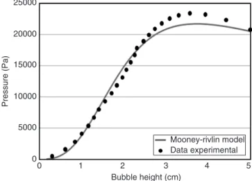
Figure 3 compares the predicted pressure versus the bubble height data at the pole of the bubble using the Mooney–Rivlin model for the experimental ABS measurements. The measurement error is less than 5% during the pressure rise. However, the numerical model for the ABS provides a better fit to the experimental data, as shown in Figure 3. It should be noted that at the maximum pressure, the bubble height is of the order of the initial membrane radius. Beyond this critical point, the height increases rapidly while the pressure falls. This unstable behavior continues until the bubble bursts.
4. COUPLING ALGORITHM
Several coupling methods for CFD and structural dynamic solvers have been developed to solve coupling problems. Classical implicit and explicit coupling are described in detail in Aquelet et al. [8], where hydrodynamic forces from the fluid solver are passed to the
Figure 2 Inflation of a flat circular ABS membrane.
25000 20000 15000 10000 5000 0 0 1 2 Bubble height (cm) Pressure (Pa) Mooney-rivlin model Data experimental 3 4 5
Figure 3 Experimental and predicted pressure versus bubble height for ABS at 145°C.
structure solver for stress and displacement computation. In this paper, a coupling method based on the contact algorithm is used, and the coupling algorithm is described in detail in Aquelet et al. [5]. Because the coupling method described in this work is based on the penalty method for contact algorithms, the contact approach is a good introduction to this method. In contact algorithms, a contact force is computed proportional to the penetration vector, which quantifies the constraint violation. In an explicit FEM method, contact algorithms compute the interface forces due to impact of the structure on the fluid, and these forces are applied to the fluid and structure nodes that are in contact to prevent a node from passing through the contact interface. One surface is designated as a slave surface and the second as a master surface in contact algorithms. The nodes that lie on both surfaces are also referred to as slave and master nodes accordingly. The penalty method imposes a resisting force on the slave node proportional to its penetration through the master segment. This force is applied to both the slave node and the nodes of the master segment in opposite directions to satisfy equilibrium.
The penalty coupling behaves like a spring system, and the penalty forces are calculated proportionally to the penetration depth and spring stiffness (see Figure 4). The head of the spring is attached to the structure or slave node, and the tail of the spring is attached to the master node within a fluid element that is intercepted by the structure.
Similar to the penalty contact algorithm, a coupling force proportional to the penetration depth is applied to both the fluid and the structure nodes.
The penalty force that is applied to both the fluid and the structure nodes in opposite directions is given by:
F= kd (8)
where k is the spring constant, and d is the relative displacement between the fluid and the structure nodes.
The accuracy of the coupling also depends on the number of coupling points used in addition to the element nodes. Additional coupling points can be positioned on the airbag membrane structure, as shown in Figure 2. A compromise must be made between too many additional coupling points, which leads to long computational times, or too few (if there are no additional coupling points), resulting in the effect of artificial leakage
d
k
Structure node Fluid node
through the membrane airbag fabric. This leakage is caused by the inflation gas source failing to connect with the coupling points and passing through the membrane airbag structure. Another possible factor is that the direction of the inflation gas source flow differs from the direction of advection, which results in mass adverted through the structure membrane.
5. NUMERICAL SIMULATIONS
To validate the formulation described above, we first consider the problem of free inflation of a viscoelastic membrane. The geometry of the structure is modeled using a quarter-symmetry model and meshed with four-node shell elements (2733 nodes and 132 shell elements) as shown in Figure 5.
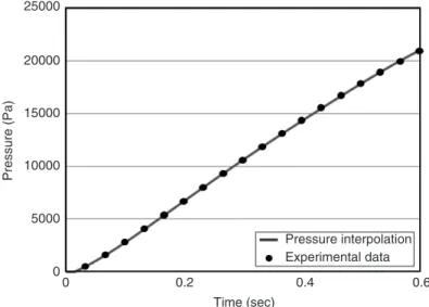
The measured pressure is interpolated by a polynomial function, as shown in Figure 6, and used in the finite element program (Lagrangian formulation) to compute the time
Pole
Figure 5 Mesh and shape of the hyper-elastic membrane.
25000 20000 15000 Pressure (Pa) 10000 5000 0 0 0.2 Time (sec) 0.4 Pressure interpolation Experimental data 0.6
evolution of the bubble height at the center pole. The predictions obtained with the Mooney-Rivlin model give almost identical results and are in agreement with the experimental data in Figure 6 at a setting temperature of 145°C. We note that the Mooney-Rivlin model predicts a similar bubble height at the pole, which is close to that of the experimental measurements. However, the model gives different results that are also close to the experimental measurements when the bubble pressure level is close to the maximum pressure reached during the experiments. This phenomenon is related to the models used and is the subject of several studies. Indeed, for these models, there exists a critical pressure beyond which the system diverges (unstable branch). The work as presented does not describe the unstable region of the solution.
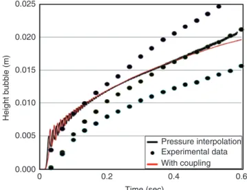
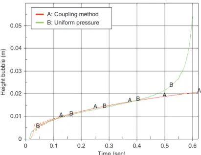
To validate the numerical results and to prove the ability of the ALE fluid structure coupling method to solve problems in cases where the classical pressure boundary conditions cannot, we use the two types of material with different Moony-Rivlin coefficients, C10 = 115590 Pa and C10 = 105010 Pa. For the first material with C10 = 115590 Pa, both formulations give the same results and show good correlation with the experimental data. The correlation can be observed in Figure 7 in which the evolution of the bubble height at the center of the membrane structure versus time is plotted for the experimental test and the numerical simulation. For the softer material with C10 = 105010 Pa, the solution from the simulation using the pressure boundary condition and no fluid becomes unstable after t = 0.6 seconds.
This instability has not been shown in our experimental tests when using this material and is due to the lack of damping that can be provided by the fluid. The missing fluid in the pressure boundary condition simulation creates a lack of damping in the system that leads the structure to numerical instability. This instability did not occur in the simulation using the fluid structure coupling because the fluid involved in the simulation has a damping effect during inflation.
For the material with C10 = 105010 Pa, the time evolution of the bubble height for both simulations is plotted in Figure 8. In this figure, the instability is evident after t= 0.6 seconds of the simulation using the uniform pressure boundary condition.
0.025 0.020 0.015 Height bubble (m) 0.010 0.005 0.000 0 0.2 Time (sec) 0.4 0.6 Pressure interpolation Experimental data With coupling
6. CONCLUSION
In this work, we present the application of a Eulerian approach for simulating the response of an isotropic and incompressible thermoplastic material. The experimental validation is performed for an ABS material in the case of free inflation of a circular membrane subject to a dynamic pressure load distribution.
An outline of the newly developed simulation procedures for membrane inflation has been detailed and explained in this paper. The most commonly used methodology for membrane inflation simulation is the uniform pressure method in which a uniform pressure is applied to the structure, and several assumptions are made regarding the inflation gas source. To conserve CPU time, the approach used in this paper combines both methods. At an early stage, the fluid structure coupling method is applied in which the fluid is modeled using the full hydrodynamic equations; at the later stage, the uniform pressure procedure is applied, and the fluid mesh and analysis are removed from the computation.
The greatest advantage of ALE is its ability to accurately model the inflation gas source, the effects of the fluid flow and the interaction with the structural parts of the model, which is especially useful in the early stages of the inflation process. Because the uniform pressure method is not accurate enough to model these situations, ALE can be used to accurately depict the initial pressure distribution inside the inflating structure. At present, simulations for the above model are run using the ALE methodology described in this article and will be published at a later date to compare the results with the Control Volume (CV) method and the test data shown in this work.
REFERENCES
[1] Erchiqui, F., Derdouri, A., Gakwaya, A., and Verron, E., Analyse expérimentale et numérique en soufflage libre d’une membrane thermoplastique, Entropie, 2001, 37(235/236), pp. 118–125. [2] Erchiqui, F., Souli, M., Ben Yedder, R., Nonisothermal finite-element analysis of thermoforming
of polyethylene terephthalate sheet: Incomplete effect of the forming stage. Polymer Engineering
and Science, 2007, 47(12), pp. 2129–2144. 0.05 A: Coupling method B: Uniform pressure 0.04 Height bubble (m) 0.03 0.02 0.01 0 0 B B B B B A A A A A 0.1 0.2 0.3 Time (sec) 0.4 0.5 0.6
[3] Khan, M., Moatamedi, M., Souli, M., Zeguer, T., Multiphysics out of position airbag simulation,
International Journal of Crashworthiness, 2008, 13(2), pp. 159–166.
[4] Hallquist, J.O., LS-DYNA theoretical manual, 1998, Livermore Software Technology Company California, USA.
[5] Aquelet, N., Souli, M., Olovson, O., Euler Lagrange coupling with damping effects: Application to slamming problems, Computer Methods in Applied Mechanics and Engineering, 2005, 195, pp. 110–132.
[6] Benso, D. J., Computational Methods in Lagrangian and Eulerian Hydrocodes, Computer
Methods in Applied Mechanics and Engineering, 1992, 99, pp. 235–394.
[7] Rivlin, R. S., Large Elastic Deformation of Isotropic Materials-IV: Further Developments of the General Theory, Phil. Trans. R. Soc., 1948, A241, pp. 379–397.
[8] N.Aquelet, M.Souli and J.Gabrys, ALE Formulation for fuel Slosh Analysis, Structural Engineering and Mechanics, an International Journal, 2003, Vol. 16, No. 4, pp. 423–440.