HAL Id: tel-02971484
https://tel.archives-ouvertes.fr/tel-02971484
Submitted on 19 Oct 2020HAL is a multi-disciplinary open access archive for the deposit and dissemination of sci-entific research documents, whether they are pub-lished or not. The documents may come from teaching and research institutions in France or abroad, or from public or private research centers.
L’archive ouverte pluridisciplinaire HAL, est destinée au dépôt et à la diffusion de documents scientifiques de niveau recherche, publiés ou non, émanant des établissements d’enseignement et de recherche français ou étrangers, des laboratoires publics ou privés.
Vision-based robotic manipulation of deformable linear
objects
Jihong Zhu
To cite this version:
Jihong Zhu. Vision-based robotic manipulation of deformable linear objects. Micro and nanotechnolo-gies/Microelectronics. Université Montpellier, 2020. English. �NNT : 2020MONTS008�. �tel-02971484�
THESIS
To obtain the doctoral degree
Delivered by University of Montpellier
Prepared within the doctoral school I2S
And from the research unit UM-CNRS LIRMM
Major in : Micro-electronical systems and robotics
Presented by : Jihong Zhu
Vision-based Robotic Manipulation
of Deformable Linear Objects
Defend on March 24, 2020 before the jury composed of
François Chaumette DR INRIA Reviewer Maximo A. Roa Researcher DLR Reviewer Véronique Perdereau PU Sorbonne Université Examiner Andrea Cherubini MCF-HDR Université de Montpellier Supervisor Philippe Fraisse PU Université de Montpellier Co-supervisor Claire Dune MCF Université de Toulon Invited David Navarro-Alarcon Assis. Prof. PolyU Hong Kong Invited
Abstract
In robotics, the area of deformable object manipulation receives far less attention than that of rigid object manipulation. However, many objects in real life are deformable. Research on deformable object manipulation is indispensable to equip robots with full manipulation dexterity. Deformable linear object (DLO) is one type of deformable objects that commonly presents in the industry and households, for instance, electrical cables for power transfer, USB cables for data transfer, or ropes for dragging and lifting equipment. In the context of H2020 VERSATILE, a project focusing on industrial automation using robots, we focus our research on DLO manipulation via visual feedback.
One characteristic of deformable object manipulation is that the object shape changes while being manipulated. Consequently, a research direction is to control the shape of the object during manipulation. We tackle the shape control problem by using vision. Ini-tially, we parameterize the shape with Fourier series, estimate and update the interaction matrix online, and finally control the DLO shape.
In the subsequent research, instead of using human-defined features for parameteriza-tion, we let the robot automatically learn feature vectors from visual data. We propose a method that allows the robot to simultaneously generate a feature vector and the interac-tion matrix from the same data. Our approach requires minimum data for initializainterac-tion. Learning and control can be done online in an adaptive manner. We can also apply the method to rigid object manipulation directly without modification.
Neither of the two frameworks requires camera calibration, and both are verified with simulation and real robotic experiments.
Another area of importance in deformable object manipulation is the utilization of external contacts. The object deformation is defined in a configuration space of infinite dimension. Nonetheless, the inputs from robots are limited. External contacts can and should be used for manipulating deformable objects. We take a practical scenario in the industry – cable routing with external contacts as the process to automate with our robot. We propose a planning algorithm that allows the robot to use contacts for shaping the cable and achieving the desired cable configuration. Real robotic experiments with different contact placement scenarios further validate the algorithms.
Résumé
En robotique, la manipulation d’objets déformables reçoit moins d’attention que celle d’objets rigides. Pourtant, de nombreux objets dans la vie réelle sont déformables. La recherche sur la manipulation d’objets déformables est indispensable pour doter les robots d’une dextérité de manipulation totale. La difficulté majeure de ce problème est que déformation de l’objet a un espace de configurations de dimensions infinie, tandis que les entrées du robots sont limitées. Dans le cadre de VERSATILE, un projet H2020 axé sur l’automatisation industrielle à l’aide de robots, nous avons axé nos recherches sur la manipulation d’objets déformables linéaires (câbles) par retour visuel.
Une caractéristique de la manipulation des objets déformables est que la forme de l’objet change pendant la manipulation. Par conséquent, un problème important consiste à contrôler la forme de l’objet pendant la manipulation. Nous avons abordé le problème du contrôle de forme en exploitant le retour visuel.
Dans un premier temps, nous avons représenté la forme de l’objet avec une série de Fourier. Nous estimons et mettons à jour la matrice d’interaction en ligne, puis nous concevons le contrôleur pour contrôler la forme.
Ensuite, au lieu d’utiliser une caractéristique définie par l’humain pour le paramétrage, nous avons laissé le robot apprendre automatiquement les vecteurs de caractéristiques à partir des données visuelles. Nous proposons une méthode qui permet au robot de générer simultanément - et à partir des mêmes données - un vecteur de caractéristiques ainsi que la matrice d’interaction. Cette méthode nécessite un minimum de données pour l’initialisation. L’apprentissage et le contrôle peuvent être effectués en ligne de manière adaptative. Nous pouvons appliquer la même méthode à la manipulation d’objets rigides, directement et sans modification.
Ces deux travaux ne requièrent aucune calibration de la caméra et ont été validés avec des expérimentations de robotique réelle.
Un autre domaine d’importance dans la manipulation d’objets déformables est l’utilisation de contacts externes pour contrôler la forme de l’objet. Les contacts externes peuvent et doivent être utilisés pour la manipulation d’objets déformables. Nous considérons un scénario fréquent dans l’industrie - l’acheminement de câbles avec des contacts externes comme processus à automatiser avec notre robot. Nous proposons un algorithme de plan-ification qui permet au robot d’utiliser des contacts pour deformer le câble et pour obtenir la configuration souhaitée. Des expériences robotiques réelles avec différents scénarios de placement de contacts permettent de valider nos algorithmes.
Acknowledgement
I would like to thank Prof. Andrea Cherubini for his patience, support and guidance during the three years of my PhD. I also want to thank my two co-supervisors, Prof. Philippe Fraisse and Prof. Andre Crosnier for their advice and feedback on my research. I would like express my gratitude to the members of my jury: Prof. François Chaumette, Prof. Véronique Perdereau, Dr. Maximo A. Roa, Dr. Claire Dune, and Dr. David Navarro-Alarcon for reading my thesis and participating in the defense. I am grateful for Dr. Benjamin Navarro, Dr. Robin Passama to their help in conducting the robot experiments. A special thank to Dr. Kai Pfeiffer whom prove-read my thesis and gave me valuable feedback.
During my PhD, I have visited ROMI lab at The Hong Kong Polytechnic University hosted by Dr. David Navarro-Alarcon for three and a half months. Despite the political instability of HongKong at that period, thanks to the kind arrangement and hospitality of David and members of the ROMI lab, I had a great and fruitful visit in Hong Kong.
I had the pleasure of meeting all the great colleagues at IDH: Dr. Stephane Caron, Dr. Sonny Tarbouriech, Dr. Osama Mazhar, Dr. Takahiro Ito, Kévin Chappellet, Anastasia Bolotnikova, Dr. Niels Dehio, Mohamed Djeha, Dr. Yukiko Osawa Akiyama, Julien Roux, Saeid Samadi and Dr. Yuquan Wang. I enjoyed our time together and thank you all for making my staying in Montpellier memorable (I hope I have included everyone). I learned much more beyond research from all of you.
A thank to Ms. Jing Dai for her encouragement, patience and support during my three year of PhD.
Last, but certainly not least, I want to thank my family whom unfortunately due to the virus outbreak are not able to attend my defense. I am grateful for their unconditional love and encouragement.
Content
1 Introduction 1 1.1 Motivation . . . 2 1.2 Contribution . . . 2 1.3 Outline . . . 3 2 Related Work 5 2.1 Deformation . . . 5 2.2 Deformation Modeling . . . 62.2.1 Pure Geometric Model . . . 6
2.2.2 Mass-Spring-Damper (MSD) model . . . 7
2.2.3 Finite Element Method (FEM) . . . 8
2.2.4 Summary . . . 8
2.3 Sensor-based Deformable Object Manipulation . . . 9
2.3.1 Tactile/force-based Manipulation . . . 9
2.3.2 Vision-based Manipulation . . . 10
2.3.3 Multi-modal Manipulation . . . 10
2.4 Deformable Linear Object Manipulation . . . 11
2.5 Visual Servoing . . . 12
3 Preliminaries 15 3.1 Visual Servoing . . . 15
3.2 Deformable Linear Objects (DLOs) . . . 16
3.2.1 Classification on Deformation Characteristics . . . 16
3.2.2 Simulation Model of Deformable Linear Object . . . 16
4 Deformable Linear Object Manipulation with Fourier-based Features 21 4.1 Introduction . . . 21
4.1.1 Problem Statement . . . 21
4.2 Our Contributions . . . 23
4.3 Methods . . . 23
4.3.1 Fourier-based Features . . . 24
4.3.2 Deformation Model Estimation . . . 25
4.3.3 Shape Servo Controller . . . 26
CONTENT 4.4 Simulation . . . 27 4.5 Robot Experiments . . . 29 4.5.1 Hardware Setup . . . 29 4.5.2 Image Processing . . . 30 4.5.3 Experiments . . . 30 4.6 Conclusion . . . 34
5 Subspace-based Object Manipulation 37 5.1 Problem Statement . . . 39
5.2 Framework Overview . . . 40
5.2.1 Problem Analysis . . . 40
5.2.2 Proposed Methods . . . 41
5.3 Methods . . . 42
5.3.1 Feature Vector Extraction . . . 42
5.3.2 Selection of the Feature Dimension k . . . 44
5.3.3 Local Target Generation . . . 44
5.3.4 Interaction Matrix Estimation . . . 45
5.3.5 Control Law and Stability Analysis . . . 47
5.3.6 Model Adaptation . . . 48
5.4 Simulation results . . . 48
5.4.1 Simulating the Objects . . . 49
5.4.2 Selecting the Feature Dimension k . . . 49
5.4.3 Manipulation of Deformable Objects . . . 51
5.4.4 Manipulation of Rigid Objects . . . 53
5.5 Experiments . . . 55 5.5.1 Image Processing . . . 56 5.5.1.1 Open Contours . . . 58 5.5.1.2 Closed Contours . . . 58 5.5.2 Vision-based Manipulation . . . 59 5.6 Conclusion . . . 63
6 Deformable Linear Object Manipulation Planning with Contacts 65 6.1 Introduction . . . 65 6.2 Problem Statement . . . 66 6.3 Our Contributions . . . 67 6.4 Framework overview . . . 67 6.5 ACMI . . . 68 6.6 Motion Primitives . . . 70 6.7 Planner . . . 71
CONTENT 6.7.2 Pre-contact Phase . . . 73 6.7.3 Post-contact Phase . . . 75 6.8 Contact Detector . . . 77 6.9 Robotic Experiments . . . 77 6.9.1 Hardware Setup . . . 77 6.9.2 Contact Localization . . . 78 6.9.3 Results . . . 80 6.10 Conclusion . . . 82
7 Conclusion and Future Work 85 7.1 Summary . . . 85
7.2 Limitation and Future Work . . . 86
Reference 88
A Appendix I
A.1 Prove of the Lemma . . . I A.2 Solution to the Optimization Problem . . . II
List of Figures
1.1 Examples of humans manipulating deformable objects. . . 1
2.1 The difference between elastic and plastic deformation by relationship be-tween stress and strain. . . 6
2.2 A demonstration of Free Form Deformation (FFD) method on an animated fish. . . 7
2.3 Mass-spring-damper model explained. . . 7
2.4 Comparison of three deformation modeling methods concerning computa-tional load and model accuracy. . . 8
3.1 Coordinate systems describe deformation. . . 17
3.2 Geometrical constraints. . . 18
3.3 Example Deformable Linear Object (DLO) shapes generated from the sim-ulator . . . 19
4.1 Cable manipulation by humans(red color marks the desired shape). . . 22
4.2 Control inputs for dual arm cable manipulation. . . 22
4.3 The cable manipulation scheme with a dual arm robot. . . 23
4.4 Manipulation simulation on the cable model. The initial and target shape are marked with dashed and solid blue, all the intermediate shapes are painted in black. The red coordinates at two endpoints specify the rotation of two end-effectors. . . 28
4.5 The cable gripper. . . 29
4.6 The hardware setup for cable manipulation. . . 30
4.7 Image processing. . . 30
4.8 Experiment 1 - Thick cable. . . 31
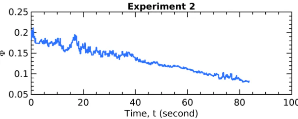
4.9 Experiment 2 - Thick cable. . . 32
4.10 Performance metric - Experiment 1. . . 32
4.11 Performance metric - Experiment 2. . . 33
4.12 Experiment 3 - Thin cable. . . 33
4.13 Performance metric - Experiment 3. . . 33
4.14 Experiment 4 - Thin cable, different starting configuration. . . 34
LIST OF FIGURES
5.1 Vision-based manipulation of rigid and deformable objects. For rigid ob-jects (left): control pose (translation and rotation). For deformable obob-jects (right): control the pose, and also shape. . . 39 5.2 Graphic representation of the vision-based manipulation problem, with its
two sub-problems, parameterization and control. . . 40 5.3 The block diagram that represents the overall framework. . . 43 5.4 Six trials conducted to test various choices of feature dimension k for a
cable. In each sub-figure, the solid red lines are the initial shapes and the dashed black are the shapes resulting from 10 random motions of the right tip (translations limited to ±5% of the length, rotations limited to ±5◦). . 49
5.5 Ten distinctive cable shapes generated by large motion: angle variation: [−π
2,
π
2], maximum translation: 106% of the cable length. . . 50
5.6 Cable manipulation with a single end-effector, moving the right tip. The blue and black lines are the initial and intermediate shapes, respectively, and the dashed black line is the target shape. The red frame indicates the end-effector position and orientation generated by our controller. . . 52 5.7 The evolution of ASE of the simulated cable manipulation using our method
against the Fourier-based method as baseline. Top: left simulation in Fig. 5.6. Bottom: right simulation in Fig. 5.6. . . 52 5.8 Comparison – for estimating s – of the receding horizon approach (RH, left)
and of the Broyden update (right, with three values of β). The topmost, middle and bottom plots show the one step prediction of s1, s2 and s3,
respectively. In all plots, the dashed red curve is the ground truth from the simulator. The plots clearly show that the receding horizon approach outperforms all three Broyden trials. . . 53 5.9 Manipulation of a rigid object with a single end-effector (red frame). The
initial, intermediate and desired contours are respectively blue, solid black and dashed black. Note that in both cases, our controller moves the object to the desired pose. . . 54 5.10 From an initial (red) pose, we generate 10 (dashed blue) random motions
of a rigid object. . . 54 5.11 Evolution of ASE of the simulated rigid object manipulation using our
method against image moments. Top: left simulation in Fig. 5.9, Bottom: right simulation in Fig. 5.9. . . 55 5.12 Progression of the auto-generated feature components (row 1, 3, 5: s1, s2,
s3) vs. object pose (row 2, 4, 6: x, y, θ). We have purposely arranged the
variables with high correlation with the same color. . . 56 5.13 Overview of the experimental setup. . . 57
LIST OF FIGURES
5.14 Open (left) and closed (right) contours can be both represented by a se-quence of sample pixels in the image. . . 57 5.15 Image processing steps needed to obtained the sampled open contour of an
object (here, a cable). . . 58 5.16 Image processing for getting a sampled closed contour: (a) original image,
(b) image after thresholding and Gaussian blur, (c) extracted contour, (d) finding the starting sample and the order of the samples. . . 59 5.17 Eight experiments with the robot manipulating different objects. From
left to right: a cable (columns 1 – 3), a rigid object (columns 4 – 6) and a sponge (columns 7 and 8). The first row shows the full Kinect V2 view, and the second and the third columns zoom in to show the manipulation process at the first and last iterations. The red contour is the desired one, whereas the blue contour is the current one. The green square indicates the end-effector. . . 61 5.18 Evolution of ei at each iteration i, for the 8 experiments of Fig. 5.17. The
black dashed lines indicate the threshold ASE = 1 pixel. The blue curves show ei until the termination condition, whereas the red curves show the
error until manual termination by the human operator. . . 61 5.19 False contour data from the image can cause noise in ASE. . . 62 5.20 Two “move and shape” experiments grouped into two rows. The desired
contour (red dotted) is far from the initial one. This requires the robot to 1) move the object, establish contact with the right – fixed – robot arm, 2) give the object the desired shape, by relying on the contact. The first column shows the starting configuration, the second column presents the contact establishment, and the third column zooms in to show the alignment. The last column shows the final results. . . 62 5.21 The evolution of ei for the experiments of Fig. 5.20. The black dashed
line indicates the threshold ASE = 1. The blue curves show ei until the
termination condition, whereas the red curves show the error until manual termination by the human operator. . . 63
6.1 Cable routing using contact. . . 66 6.2 A contact-based manipulation example to illustrate the problem. The
or-der of the contacts is given by the number besides each contact. This information is provided a priori to the robot. . . 67 6.3 Example of a circular object in contact with a cable. The green vector is a
candidate direction of relative object/cable motion. Many other directions are possible. . . 68
LIST OF FIGURES
6.4 The Angular Contact Mobility Index (ACMI) in four contact cases, (a): no contact; (b): point contact; (c): curved contact with 0 < ψ ≤ π; (d):
curved contact with π < ψ ≤ 2π. . . 69
6.5 The effect of rotation on the ACMI . . . 70
6.6 The effect of sliding on the ACMI. . . 70
6.7 Motion primitives: (a). End-effector F holds while end-effector M rotates the cable, (b). End-effector F releases while end-effector M pulls the cable. 71 6.8 Flow chart depicting the steps needed to reach the final target by contact-based manipulation with n contacts. . . 72
6.9 Position planning for a single contact. . . 72
6.10 Multiple contacts planning example. The order of the contacts is presented by the numbering besides each contact, and known by the robot, which can then compute the initial pose. . . 74
6.11 Rotation to reach the contact. . . 74
6.12 Full rotational motion planning. . . 76
6.13 The pull can be regarded as a sliding motion. . . 76
6.14 Extraction of the cable ends and the contact. . . 78
6.15 Designs of the two end-effectors. . . 79
6.16 Setup and coordinate frames. . . 79
6.17 Total manipulation time for each scenario. Single contact cases: 1,2. Two contacts cases: 3-5. Three contacts cases: 6-8. . . 81
6.18 Final cable configurations in six of the eight scenarios. . . 81
6.19 (a): Planned motion for scenario 8; (b): Example calculation of the ACMI of contact 1 after the robot motion. . . 81
6.20 The nominal ACMI and the ACMI after the manipulation. . . 82
6.21 Manipulation experiments with more than one contact. Contacts are de-noted with black dots, and the nominal cable configuration is drawn with solid (2 contacts) and dashed (3 contacts) lines . . . 83
List of Tables
3.1 DLO classification with example objects reproduced from [Henrich et al.,
1999]. . . 16
5.1 Explained variance Υ(k) for the 6 trials with small motion. . . 50
5.2 Explained variance Υ(k) computed with large motion. . . 50
List of Acronyms
ACMI Angular Contact Mobility Index AFFD Animated Free-Form Deformation CAD Computer-aided Design
DFFD Discontinuous Free Form Deformation DLO Deformable Linear Object
DVS Direct Visual Servoing
EFFD Extended Free Form Deformation FEM Finite Element Method
FFD Free Form Deformation HSV Hue-Saturation-Value
IBVS Image-based Visual Servoing MSD Mass-Spring-Damper
PBVS Position-based Visual Servoing PCA Principal Component Analysis RGB Red-Green-Blue
ROI Region of Interest SER Shape Error Reduction
Chapter 1
Introduction
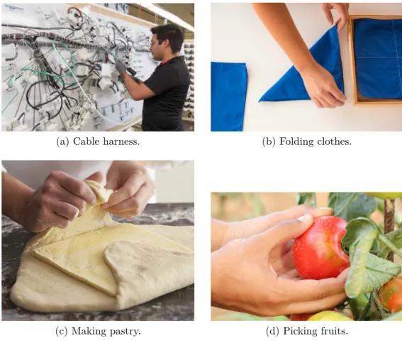
Humans are dexterous in manipulation. From an evolution perspective, the transition to bipedal that free both hands for manipulation contributes significantly to human intelli-gence [Newman and Newman, 2015]. Similarly, for robots to develop intelligent behavior, one of the critical aspects is manipulation. Robotic manipulation, as a subfield of robotics, has been studied for over four decades now. Most of the works assume that the object is rigid – the object’s shape stays unchanged during manipulation. However, humans also manipulate deformable objects, i.e., objects whose shape changes cannot be neglected. Figure 1.1 shows multiple examples of humans manipulating deformable objects. The ability to manipulate deformable objects is indispensable for robots to achieve full ma-nipulation dexterity.
(a) Cable harness. (b) Folding clothes.
(c) Making pastry. (d) Picking fruits.
Figure 1.1: Examples of humans manipulating deformable objects.
Introduction 1.1. Motivation
modeling, sensing, and control. We elaborate on these challenges one by one.
The modeling of deformable objects is a research topic in computer graphics. A re-alistic model encompassing physical properties is often computationally heavy and not suitable for real-time simulation [Moore and Molloy, 2007]. Sensing of deformation is usu-ally done with vision or force. The extraction of the shape changes from sensory data is non-trivial. Last but not least, deformation imposes new problems in manipulation con-trol, as the shape of the object is not static anymore. One prominent problem with control is underactuation. The inputs from the robots are limited, but the object’s deformation has infinite degree of freedom (DoF).
Needless to say, we cannot tackle all three challenges within this thesis. Rather, we focus on one specific topic that is the vision-based shape control of deformable linear objects (DLOs), such as cables, ropes, wires to name a few. We start with a framework for dual arm shape control, and then a generalized framework for both rigid and deformable object manipulation is formulated. We explore the use of environmental contacts in deformable object manipulation that enables robots to perform cable routing tasks.
1.1
Motivation
Robotic manipulation research has resulted in a huge number of methods and algorithms. Only a small fraction of these are dedicated to deformable objects. Automatic manip-ulation and shaping of deformable objects opens new doors for robotic applications in areas like: surgical operation [King et al., 2009], agriculture [Li et al., 2011], food mak-ing [Yamaguchi and Atkeson, 2016], household services [Bersch et al., 2011] and industrial automation [Qin et al., 2019].
This thesis is supported by the H2020 VERSATILE project1 – a project which aims at
developing advanced robotic manipulation capabilities in industrial environments. One of the most common deformable objects used in the industrial setting are DLOs that enable data and power transfer. We usually need to manage them in an organized way, which usually involves conforming them to designated shapes or configurations. Therefore, we work on shaping DLO via visual feedback. Taking a step forward, we also develop a generalized framework for both rigid and deformable object manipulation using vision.
1.2
Contribution
This thesis contributes to the state-of-the-art in deformable object (mainly DLOs) ma-nipulation in terms of novel algorithms and applications for shape control, specifically:
• A cable shape control algorithm for a dual arm robot is presented in Chapter 4. The
1
Introduction 1.3. Outline
chapter is based on the paper [Zhu et al., 2018] “Dual-arm Robotic Manipulation of Flexible Cables” 2.
• A unified object manipulation framework via visual feedback is presented in Chap-ter 5. The chapChap-ter is based on [Zhu et al., 2020b] “Vision-based Manipulation of Deformable and Rigid Objects Using Subspace Projections of 2D Contours”3, under
review.
• A robotic manipulation planning utilizes environmental contacts for shaping DLOs is presented in Chapter 6. The chapter is based on the paper [Zhu et al., 2020a] “Robotic Manipulation Planning for Shaping Deformable Linear Objects With En-vironmental Contacts” 4.
The videos of the experiments are all available on the Interactive Digital Humans (IDH) group’s YouTube channel:
• Cable shape control: http://y2u.be/DPl_d7lbL84
• Unified object manipulation: http://y2u.be/gYfO2ZxZ5KQ
• Contact-based planning: http://y2u.be/7CdNQ4R_wT0
The work of this thesis also motivated a workshop at IROS 2020 on “Managing De-formation: A Step Towards Higher Robot Autonomy” 5 where I am the main organizer.
1.3
Outline
The rest of the thesis is organized as follows:
Chapter 2: provides related works on deformable object manipulation and
vision-based control.
Chapter 3: introduces the basic concept of visual servoing, which we adopt in the
rest of this thesis. In addition, it provides a classification of DLOs based on [Henrich et al., 1999]. In the last section, we develop a DLO model for validation of the proposed algorithms.
Chapter 4: discusses dual arm vision-based DLO manipulation using Fourier
param-eterization based on [Zhu et al., 2018].
Chapter 5: discusses a unified vision-based scheme for manipulation of both rigid
and deformable object. The chapter is based on [Zhu et al., 2020b].
2 https://ieeexplore.ieee.org/stamp/stamp.jsp?arnumber=8593780 3 https://hal.archives-ouvertes.fr/hal-02558064/ 4 https://hal.archives-ouvertes.fr/hal-02303257/ 5 https://sites.google.com/view/madef-iros2020/home
Introduction 1.3. Outline
Chapter 6: introduces a planning framework that allows robots to perform the cable
routing task with environmental contacts. The chapter is based on [Zhu et al., 2020a].
Chapter 2
Related Work
In this chapter, we review works that relate to the topic of this thesis. In the first section, we explain the concept of deformation. Although in this thesis we adopt a model-free approach for manipulation, it is crucial to review the works on deformation modeling, thus give the rationale behind our choice. A survey on deformation modeling is presented in Section 2.2. We dedicate Section 2.3 to previous works on sensor-based deformable object manipulation. Section. 2.4 presents works on DLO manipulation. Since two manipulation frameworks (Chapter 4 and 5) in this thesis are based on visual servoing, in Section 2.5, we review research on visual servoing.
2.1
Deformation
Deformation in the context of the thesis denotes changes in the shape or size of an object due to an applied force1. Depending on the resulting shape of the object after removing
the force, we can classify deformation as plastic, elastic, or elasto-plastic.
A plastic deformation means that the object remains in its deformed state (shape) after the force is relaxed. An elastic deformation, on the contrary, entails that the object returns to its original state (shape) after having removed the force. The elasto-plastic deformation is somewhere in between: the object does not return to its original shape but also does not stay in its deformed shape.
Stress (σ) and strain (ǫ) can describe deformation. Stress refers to the force applied over an area and is measured in pressure units (N · m−2). Strain measures the change in length or angle of the object due to such force.
As shown in Fig. 2.1, the elasticity in deformation is measured by Young’s modulus E [Askeland and Phule, 2003], which induces a linear relationship between stress and strain [Callister et al., 2007]:
σ = Eǫ (2.1)
The Young’s modulus measures stiffness of the object. A large E implies high stiffness and vice versa. It is a vital parameter to model elastic deformation, yet geometrical linearity is not appropriate for large deformations, because only small deformations can
1
Related Work 2.2. Deformation Modeling Strain S tr es s
Red: Elastic Region
Green: Plastic Region
Figure 2.1: The difference between elastic and plastic deformation by relationship between stress and strain.
be modeled accurately [Nealen et al., 2006]. In the next section, we will discuss the means of modeling deformation.
2.2
Deformation Modeling
Deformation modeling is not a subject of robotics but rather of computer graphics. How-ever, since in this thesis we are dealing with deformable objects, it is necessary to review models of deformation. In this section, we present the three most common models of deformation: i) pure geometric, ii) mass-spring-damper, iii) finite element method.
2.2.1
Pure Geometric Model
A pure geometric model, as its name suggests, does not take into account the physics that govern the deformation. The model consists of no knowledge of the mechanical property of the object. The model accuracy is compromised for fast computation.
The geometric model normally uses a set of control points to construct curves or surfaces. These control points are fitted with different spline functions, such as: Bezier curve, B-spline, and Fourier series among others. Examples of these methods can be found in [Bartels et al., 1987]. Instead of fitting control points, [Barr, 1987] introduced operators that can be applied to control points hierarchically to obtain deformation. A generalized method is later proposed by [Sederberg and Parry, 1986], which is known as the FFD method. The FFD encloses the object with a hull (usually a cube). The object deforms as the hull reshapes by the control points (see Fig. 2.2).
The FFD method received considerable attention in the research community. Re-searchers proposed several modified versions of FFD. Coquillart developed the Animated Free-Form Deformation (AFFD) [Coquillart and Jancene, 1991] and the Extended Free Form Deformation (EFFD) [Coquillart, 1990] that allowed more intuitive control over
Related Work 2.2. Deformation Modeling
(a) Original fish and en-closed cube with control points
(b) Deformed fish by pulling the control points
(c) Deformed fish by pulling the control points
Figure 2.2: A demonstration of FFD method on an animated fish.
deformation. More recently, [Schein and Elber, 2004] developed the Discontinuous Free Form Deformation (DFFD) technique to better incorporate discontinuities in deformation. The FFD and its extensions are typical geometric deformation models. They are used in Computer-aided Design (CAD) applications as a geometric sculpting tool. Since there is no information about the object’s physical properties, the obtained model is not able to simulate the object realistically for real-time control purposes. For instance, the deformed fish in Fig. 2.2c in not realistic but can be obtained by manipulating the control points.
2.2.2
Mass-Spring-Damper (MSD) model
One simple dynamical model is the Mass-Spring-Damper (MSD) model. Instead of only considering the geometric points as in the previous section, the deformation model is represented by a collection of discretized point masses connected with springs and dampers in between (Fig. 2.3).
(a) Mass-spring-damper model (b) Point masses connected by mass-spring-damper
Related Work 2.2. Deformation Modeling
The MSD model was initially used in facial modeling in computer graphics [Platt and Badler, 1981], [Waters, 1987]. Later, it was applied to the simulation of skin and muscle [Chadwick et al., 1989]. It can also be used to create animated locomotion for snakes, worms [Miller, 1988] and fishes [Tu and Terzopoulos, 1994]. A MSD-based cloth model is proposed in [Breen et al., 1994].
The MSD systems are intuitive, generally easy to implement, and computationally efficient, making real-time animations possible. The main drawback associated with using MSD systems is that the discrete model imposes significant approximations of the true physics that would occur in a continuous body [Moore and Molloy, 2007].
2.2.3
Finite Element Method (FEM)
Finite element methods divide the object into a discrete mesh of smaller components re-ferred to as finite elements. The more elements the model has, the more computation is needed, and the more accurate the model will be. Compared to MSD methods which directly employ a discrete model, Finite Element Method (FEM) starts with continuous partial differential equations (PDEs) describing the deformation. These are then dis-cretized over the single finite elements. The FEM result in a more accurate model, yet more computationally demanding.
In deformation modeling, the FEM is widely applied, to name a few applications: skin simulation [Benítez and Montáns, 2017], muscle [Chen, 1991], shape editing [Celniker and Gossard, 1991], and cloth modeling [Etzmuß et al., 2003]. FEM is used in areas where model accuracy is critical, such as surgical simulation [Berkley et al., 1999].
2.2.4
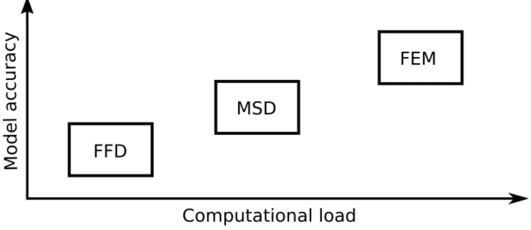
Summary
The above three methods for deformation modeling are ranked by model accuracy and computational load in Fig. 2.4.
Computational load M o d el a c c u ra c y FEM MSD FFD
Figure 2.4: Comparison of three deformation modeling methods concerning computational load and model accuracy.
Related Work 2.3. Sensor-based Deformable Object Manipulation
The FFD and its variations, since no physical property is involved, are not suitable for model-based robotic manipulation control of deformable objects. The two other methods are capable of simulating deformable objects accurately. However, the model needs to be identified before applying it to the real-time manipulation control. For different objects, a re-identification is required. If these methods are employed, we will need to construct offline different models before manipulating different objects. Therefore, instead of find-ing a global deformation model for robotic manipulation, we tend to favor model-free approaches. One prominent paper in this direction is [Berenson, 2013], where the au-thor derived the interaction matrix based on the concept of diminishing rigidity. More recent approach, [Hu et al., 2019] learned the mapping between the robotic end-effector’s movement and the object’s deformation measurement with Gaussian process regression. Model-free approaches produce more general manipulation schemes with minimum offline modeling required. Besides, they are much less computationally demanding than MSD or FEM-based approaches.
Nevertheless, they also have their drawbacks, which we will later discuss in detail in Chapter 4 and 5.
2.3
Sensor-based Deformable Object Manipulation
Deformable object manipulation is an emerging area of research in the robotics community. We distinguish different manipulation approaches depending on the sensor feedback.
2.3.1
Tactile/force-based Manipulation
As mentioned in Section 2.1, deformation is a result of force applied to the object. There-fore, works have been done in manipulation based on tactile/force feedback.
Tactile information can be used to deduce deformation and thus feedback to control manipulation [Delgado et al., 2015]. Moreover, it can detect/correct slips and regulate grasping forces while manipulating deformable objects with a dynamic center of mass [Kaboli et al., 2016].
Due to critical tactile information produced during manipulation, research has been done in designing novel tactile sensors that can distinguish rigid and deformable objects [Drimus et al., 2014].
Force sensing could be useful in detecting vibration. For example, [Yue and Henrich, 2002] achieved fast manipulation under vibration with force/torque feedback. Some of the force-based methods make use of machine learning to derive manipulation strategies. A neural network was trained in [Howard and Bekey, 2000] to model the effect of force on deformable object manipulation. Recently, Lee et al. proposed a force-based manipulation skill learning approach for deformable object manipulation [Lee et al., 2015].
Related Work 2.3. Sensor-based Deformable Object Manipulation
Since tactile and force information are often only locally available at contact points, these approaches are more focused on grasping the object or in-hand manipulation of the object. An object shape, instead, can represent the global deformation of that object. Shapes are usually observed via vision, therefore in the next section, we review works in vision-based manipulation.
2.3.2
Vision-based Manipulation
Another obvious indication of deformation is shapes. While force/tactile based approaches usually require a model to infer deformation as an outcome of the force applied, vision directly observes the resulting shape changes.
One of the initial works on the manipulation of deformable objects via visual feedback is presented in [Inoue, 1984] to solve a knotting problem. Smith et al. developed a relative elasticity model such that vision can be utilized without a physical model for the manipulation task [Smith et al., 1996]. Acker and Henrich applied vision to detect contact state changes [Acker and Henrich, 2003]. A hierarchical self-organizing neural network was developed along with vision to select proper grasping points on the deformable objects [Foresti and Pellegrino, 2004]. In recent research, Nair et al. combined learning and visual feedback to manipulate ropes [Nair et al., 2017]. Navarro-Alarcon et al. presented several papers focusing on vision-based deformable object manipulation. In his initial work, [Navarro-Alarcon et al., 2013a] employed the Broyden update rule for interaction matrix estimation, and a nonconservative Hamiltonian dynamical system to compute the state feedback laws. A passivity-based controller was proposed in [Navarro-Alarcon et al., 2013b] to deform object under inaccurate interaction matrix estimation. In this later work, [Navarro-Alarcon and Liu, 2014] considered 6 DoF motion of the robot manipulator for the manipulation task. However, the method used geometric features such as points, lines, and curvature to name a few, which could only express certain kinds of deformation. Taking a step further, in his latest work, [Navarro-Alarcon et al., 2016] proposed a generalized feature based on Fourier series for manipulation. [Laranjeira et al., 2017] proposed a vision-based management framework for tethers that link terrestrial mobile robots. Recently, [Chi and Berenson, 2019] introduced a robust vision-based sensing of deformable objects considering occlusion using Coherent Point Drift.
Other than receiving information locally, vision can provide global information on object deformation. Due to this aspect, vision often contains noisy data that needs pre-processing to yield a reasonable estimate of the deformation.
2.3.3
Multi-modal Manipulation
Since the problem of deformable object manipulation is complex, some researchers have also considered utilizing multiple sensor modalities for manipulation.
Related Work 2.4. Deformable Linear Object Manipulation
The author of [Hirai et al., 2001] presented one of the first multi-modal approaches for deformable object manipulation, where they used both force and vision information. In [Luo and Nelson, 2001], to observe changes in shapes, the authors applied an active contour method and a FEM model with force feedback, to predict deformation. Later [Huang et al., 2005] introduced a position/force hybrid control method that incorporates visual information with force control for flexible tool manipulation.
The multi-modal method is a promising research direction. Nonetheless, how to com-bine different sensor modalities to produce accurate state estimation of the deformable objects for feedback control is one of the challenges in this area of research.
2.4
Deformable Linear Object Manipulation
In this section, we review the type of research that is closely related to this thesis – DLO manipulation.
Compared with general deformable objects, DLOs are simpler to model. We dis-tinguish two kinds of models: dynamical and topological. The former embeds physical properties of the objects and the latter concerns only the topology.
A dynamic model considering bend, twist, and extensional deformations is proposed in [Wakamatsu et al., 1995] using differential geometry. The shape of the DLO is solved by an optimization on the total energy under constraints. Later, the authour of [Wakamatsu and Hirai, 2004] used this model for grasping and manipulation of DLOs. The modeling can also be solved with FEM. The dynamic 2D deformation of an inextensible linear object was formulated using FEM in [Huang et al., 2008]. The method was claimed to be computationally faster than the differential geometry method mentioned previously. The author of [Yoshida et al., 2015] applied FEM for ring-shape objects for assembly tasks. Dynamical models can compute the shape of the DLO under constraints. These models are used when shape matters during manipulation.
Sometimes in DLO manipulation, topology rather than the exact shape is of interest, for instance, tying and untangling DLOs. Knot theory [Murasugi, 2007] can be used to develop a topological model for DLOs to solve the knotting problem. At an initial step in this direction, [Phillips et al., 2002] proposed a simple model for knot tying. In this model a rope in a loosely knotted configuration was pulled tight, and the knot was preserved, using an impulse model for collision handling. The rope was modeled as a spline of linear springs, with spheres placed on the control points to represent the rope volume. The spheres tend to bunch up or stretch apart during the simulation, due to the spring model, but collision handling did prevent the rope from passing through itself. In addition, the model did not operate in real time. The author of [Brown et al., 2004] took a step forward and formulated a knotting simulator capable of real-time simulation. These simulators contributed to the later works on robot motion planning to the tying
Related Work 2.5. Visual Servoing
and untangle the DLO [Moll and Kavraki, 2006], [Ladd and Kavraki, 2004]. Researchers also explored learning in solving the knotting problem. The author of [Takamatsu et al., 2006] employed a learning from observation (LFO) paradigm for knot tying tasks. The robot learned a set of motions needed from human demonstration to complete the task. Knotting is of practical interest in medical and construction applications. A robotic knot tying framework in surgeries was presented in [Kang and Wen, 2002]. Quadrocopters performed aerial knot-tying which is an essential task in the aerial assembly of tensile structures [Augugliaro et al., 2015].
Several research works are dedicated to manipulation planning of DLOs: A collision-free path planner was developed in [Lamiraux and Kavraki, 2001] using a randomized algorithm. A planner in [Moll and Kavraki, 2006] computed a path in the shape space from one minimal energy curve to another while satisfying environmental constraints. Bretl and McCarthy showed that the shape space of an elastic rod is a six-dimensional smooth manifold [Bretl and McCarthy, 2014]. Later, the authors of [Borum and Bretl, 2015] took a step forward and proved the path-connectedness of this space.
2.5
Visual Servoing
Visual servoing or vision-based control is a crucial area of research in robotics. The use of vision enables robots to observe and actively react to the environment. The visual servoing scheme transforms visual information into a feature vector. The difference between the current feature vector value and the desired one produces an error term. Then the scheme tries to minimize this error by robot motion.
One of the first papers on visual servoing dates back to [Shirai and Inoue, 1973]. Since then, considerable effort has been made in the area. We refer interest readers to [Chaumette and Hutchinson, 2006a] and [Chaumette and Hutchinson, 2007a] for a com-prehensive tutorial on this subject. There are two classes of the visual servoing scheme: Image-based Visual Servoing (IBVS) and Position-based Visual Servoing (PBVS). The former uses the image data directly to generate feature vectors while the latter uses image data for estimation of 3D position in space and then use it for the servoing task. Here we focus on IBVS, which is the method adopted in our research.
Some commonly selected geometric features for IBVS are points, lines and moments [Chaumette, 2004]. Kernel-based visual servoing [Kallem et al., 2007] combined feature tracking and control using spatial sampling kernels to generate features to design feed-back controllers, thus eliminates the need for image processing to obtain features. Similar methods are referred to as Direct Visual Servoing (DVS). The DVS has received con-siderable attention. Several high impact works were published in the field. Collewet et al suggested using luminance of all pixels on the image for visual servoing [Collewet et al., 2008], [Collewet and Marchand, 2011]. In the subsequent research, photometric
mo-Related Work 2.5. Visual Servoing
ments are considered as a new feature for visual servoing [Bakthavatchalam et al., 2013], [Bakthavatchalam et al., 2018]. In the latest research, [Marchand, 2019] proposed a DVS approach based on the Principal Component Analysis (PCA).
We intend to solve deformable object manipulation by IBVS. Therefore, methods and algorithms are developed in the framework of IBVS considering this context.
The authors of [Navarro-Alarcon and Liu, 2017] introduced the concept of shape ser-voing as a sub-field of visual serser-voing. The shape serser-voing research considers utilizing visual feedback for controlling the shape of the object. We extended the approach to consider a dual arm setup in [Zhu et al., 2018]. An expository paper on the topic is also available in [Navarro-Alarcon et al., 2019].
In this thesis, we extend and propose new algorithms and frameworks in shape servo-ing.
Chapter 3
Preliminaries
In this chapter, we give a general introduction to key concepts of the thesis. Section 3.1 introduces a generalization of the visual servoing scheme [Chaumette and Hutchinson, 2006a], which we follow to develop our shape servoing algorithms. Section 3.2 addresses the concept of DLOs and their classification. We develop a model for verifying our shape servoing framework and present it in Section 3.2.2.
3.1
Visual Servoing
A unified description for all vision-based control is to minimize the error term e(t) in:
e(t) = s(m(t), a) − s∗, (3.1) where s is the feature vector that consists of image measurements m and additional knowledge of the system a [Chaumette and Hutchinson, 2006a].
Visual servoing approaches differ in the selection of the feature vector s. Once selected, we compute the relationship between robot spatial velocity ˙r and resulting time derivative of ˙s:
˙s = L ˙r, (3.2)
in which L is the interaction matrix (or feature Jacobian) relating the two. Given a time instant δt, we can write the discretized version of (3.2) as:
δs = Lδr, (3.3)
where δs = ˙sδt and δr = ˙rδt correspond to the step changes in robot motion and feature vector respectively.
In general, it is not possible to obtain perfectly the interaction matrix. Thus its approximation ˆL is often used to formulate control:
˙r = −λ ˆL†˙e, (3.4) where †represents the Moore-Penrose pseudo-inverse. Similarly the discretized version of
Preliminaries 3.2. Deformable Linear Objects (DLOs)
(3.4) is:
δr = −λ ˆL†e, (3.5)
The shape servoing problem [Navarro-Alarcon and Liu, 2017] also falls into the for-mulation of (3.1). We will discuss it in detail in Chapter 4 and 5.
3.2
Deformable Linear Objects (DLOs)
Deformable Linear Objects commonly appear in household and industrial environment, for instance, ropes, elastic rods, beams, and cables to name a few. The term “Linear” refers to the shape of the object can be simplified as a curve/line as one dimension of the object is dominant in length.
3.2.1
Classification on Deformation Characteristics
Henrich et al. proposed a classification of DLOs based on their deformation characteristics [Henrich et al., 1999]:
Table 3.1: DLO classification with example objects reproduced from [Henrich et al., 1999].
N E- E+ P- P+ Description no defor-mation low elastic deforma-tion high elastic deforma-tion low plastic deforma-tion high plastic de-formation Linear objects examples short steal tubes short spring steal long spring steal short iron wires ropes
The categorization between a + or - in Tab. 3.1 is dependent on whether gravity alone can make the object deform. If it is the case, then the object is in the + category; otherwise, it belongs to the - category.
The DLOs used in our experiment are in the E+ category (marked with red color on the table).
3.2.2
Simulation Model of Deformable Linear Object
We adopt the model based on differential geometry [Wakamatsu and Hirai, 2004], where the shape of the DLO can be solved by a constrained optimization. We simplify it for our manipulation task by constraining the DLO to a 2D plane.
The deformation is expressed in terms of frame fields. Assume the total length of the linear object is L. P (s) is a point at distance s from the left end of the linear object. In Fig. 3.1, let O − xy be the fixed world coordinate on the plane. P − ζξ is the local
Preliminaries 3.2. Deformable Linear Objects (DLOs)
coordinate attached to point P (s). Angle φ(s) specifies the rotation of P − ζξ around the world frame z axis.
(a) Natural state (b) Deformed state
Figure 3.1: Coordinate systems describe deformation.
The rotational matrix that transforms O − xy into P − ζξ is:
A(φ) = cos φ − sin φ sin φ cos φ Let ω = dφ
ds be an infinitesimal rotation at point P (s). Then the following equation is
satisfied: dA ds = A 0 −ω ω 0
Since A is an orthonormal matrix, we have then:
0 −ω ω 0 = AT dA ds = cos φ sin φ − sin φ cos φ − sin φdφ ds − cos φ dφ ds − cos φdφds − sin φdφds
The underlying principle in DLO modeling is that the potential energy of a deformable object reaches its minimum for the object’s static shape [Wakamatsu et al., 1995]. In the 2D case, the total potential energy of the DLO is just the fluexual energy:
U = Uflex,
which can be computed by integration:
Uflex = 1 2 Z L 0 Rf( dφ ds) 2ds,
with Rf a constant representing the flexural rigidity of the object.
Let us express φ(s) by a linear combination of basic functions e(s):
φ(s) = n
X
i=1
Preliminaries 3.2. Deformable Linear Objects (DLOs)
The basic function e(s) can be defined as:
e1 = 1, e2 = s, e2i+1= sin 2πis L , e2i+2= cos 2πis L .
During manipulation, four geometry constraints can be imposed on the DLO. They are the distance between two manipulation ends along the x and y axis: lx and ly; plus two
rotational angles at the two ends φ(0) and φ(L) as shown on Fig. 3.2. The four constraints yields:
lx = Z L 0 cos(φ(s))ds, ly = Z L 0 sin(φ(s))ds, φ(0) = θ1, φ(L) = θ2, (3.7)
Figure 3.2: Geometrical constraints.
The final optimization problem is then:
min a 1 2 Z L 0 Rf( dφ(s) ds ) 2ds (3.8)
subject to equality constraints in (3.7).
By solving the optimization problem, we obtain the shape of a DLO under specific manipulation constraints. We solve the optimization problem by CasADi [Andersson
Preliminaries 3.2. Deformable Linear Objects (DLOs)
(a) (b) (c) (d)
(e) (f) (g) (h)
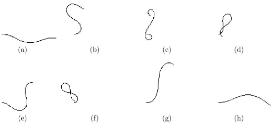
Figure 3.3: Example DLO shapes generated from the simulator
et al., 2019]. Figure 3.3 shows examples of shapes generated using our DLO simulator. Each cable is of unit length and represented by K = 100 points (tunable in the simulator). The simulator will be used later for testing the shape servoing frameworks 1. Note that
it is used only for verification of shape servoing algorithms, not for real-time simulation of any DLO.
1
The 2D simulator of the DLO was made publicly available at https://github.com/Jihong-Zhu/ cableModelling2D
Chapter 4
Deformable Linear Object
Manipulation with Fourier-based
Features
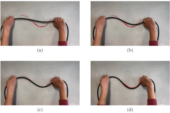
As a starting point of the research, we focus on shaping DLO with a dual arm robot. We aim at a shaping task which humans can perform with both hands (see Fig. 4.1). In this chapter, we adopt the method in [Navarro-Alarcon and Liu, 2017] and propose a framework to deform a DLO to a target shape via visual feedback. For better readability, we replace the term DLO with cable in this chapter.
4.1
Introduction
Given a (reachable) desired cable shape, a human can deform the cable into such shape relying on visual feedback without the need for re-grasping (see Fig. 4.1). This task is easy for a human to do without even knowing the internal dynamics of the cable. For robots, it remains a challenge.
4.1.1
Problem Statement
Let us consider a dual arm robot manipulating a cable on a 2D plane. The cable is a system with unknown dynamics that accepts inputs from the robot. Each robot end-effector applies three incremental inputs, respectively: two translations in the manipulation plane,
δx and δy, and one rotation δθ along the axis perpendicular to the manipulation plane
(see Fig. 4.2). The total number of inputs from the robot is six, specifically:
δr = [δx1 δy1 δθ1 δx2 δy2 δθ2]T ∈ R6. (4.1)
A static camera continuously observes the shape of the cable. The cable shape in the camera image is represented as C = [u, v]T ∈ R2×K, where u ∈ RK and v ∈ RK are
image coordinates of pixels sampled along the cable. We represent the desired cable shape by C∗.
Deformable Linear Object Manipulation with Fourier-based Features 4.1. Introduction
(a) (b)
(c) (d)
Figure 4.1: Cable manipulation by humans(red color marks the desired shape).
robot manipulator initial position
robot manipulator final position cable final shape cable initial shape
Deformable Linear Object Manipulation with Fourier-based Features 4.2. Our Contributions
The problem we address is to use the control inputs δr to drive the cable from its initial shape C0 to the desired shape C∗ using visual feedback.
4.2
Our Contributions
We propose a shape servoing algorithm to complete the task depicted in Fig. 4.1 for a dual arm robot. A receding window approach ensures that the most recent data is used for computing the interaction matrix relating the robot inputs and the shape changes. Then this interaction matrix is used to compute the robot inputs. The algorithm is validated by simulations and on a real robot setup.
4.3
Methods
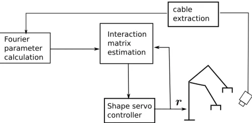
To tackle the problem stated above, we first transform the cable shape into a feature vector. After parameterizing the shape, we model the relationship between the robot motion and the changes in the shape parameters locally by an interaction matrix. The final step is to derive the control strategy to deform the cable into the desired shape based on the interaction matrix. In this section, we describe each sub-task sequentially. The overall shape servoing scheme is explained in Fig. 4.3.
cable extraction Shape servo controller Interaction matrix estimation Fourier parameter calculation
Deformable Linear Object Manipulation with Fourier-based Features 4.3. Methods
4.3.1
Fourier-based Features
The ith sample point c(i) = [u(i), v(i)]T, i = 1, 2, . . . , K in C can be approximated using
a Nth ordered Fourier series:
u(i) = N X j=1 [aj bj] cos(jρi) sin(jρi) + e, v(i) = N X j=1 [cj dj] cos(jρi) sin(jρi) + f, (4.2) with ρi = (i − 1) π K.
The feature vector s in (4.2) is:
s= [a1 b1 . . . aN bN e c1 d1 . . . cN dN f ]T ∈ R4N +2. (4.3)
This will later be used both in deformation model estimation and control. Below we show how to solve for s given image data.
We can rewrite (4.2) as:
c(i) = u(i) v(i) = fT(i) 0 0 fT(i) s. (4.4)
In (4.4), f (i) are the harmonics terms defined as:
f(i) = [cos ρi sin ρi . . . cos(N ρi) sin(N ρi) 1] ∈ R2N +1. (4.5)
Using all K samples in C, we have:
C′ = Gs, (4.6) with: C′ = [c(1)T c(2)T . . . c(K)T]T ∈ R2K, G= f(1) 0 0 f(1) ... ... f(K) 0 0 f(K) ∈ R2K×(4N +2).
Deformable Linear Object Manipulation with Fourier-based Features 4.3. Methods
be solved by linear least squares:
s= G†C,
where † represents the Moore-Penrose pseudo inverse: G† = (GTG)−1GT.
To ensure the pseudo inverse of G exists we need that:
rank(G) = 4N + 2 (4.7)
is fulfilled. A necessary condition for (4.7) is:
2K ≥ 4N + 2.
So we need to collect at least 2N + 1 samples to compute the feature vector.
4.3.2
Deformation Model Estimation
Feature vector s describes the cable shape. Locally, a small movement of the robot pro-duces a tiny change in the cable shape, hence on the feature vector. From this observation, at a given operating point, we can linearize the deformation model as:
δs = Lδr. (4.8)
Vector δr ∈ R6 corresponds to robot motion, and δs ∈ R4N +2 is the corresponding change
in the feature vector; L ∈ R(4N +2)×6 is the local deformation matrix.
For the ith element of s, we can write:
δsi = δrTlTi ,
where li is the ith row of L. Its transpose liT ∈ R6.
To estimate lT
i , at the current instance tm, we collect M prior data of δsi and δrT
while the robot is moving:
σi = δsi(t1) δsi(t2) ... δsi(tM) ∈ RM, R = δrT(t 1) δrT(t 2) ... δrT(t M) ∈ RM×6.
In the above equations, each si(tj) is the corresponding feature vector after robot motion δrT(t
j). Using R and σi we have:
Deformable Linear Object Manipulation with Fourier-based Features 4.3. Methods
and we can estimate li as
ˆ
lTi = (R T
R)−1RTσi. (4.10)
Therefore, we can estimate every row of L. To successfully estimate L, the following conditions must be satisfied:
• R must have full row rank.
If the condition is not satisfied, RTR in (4.10) will be singular. In practice, this
condition infers that within the time window {t1 − tN}, it is necessary that the robot
moves in all directions and rotates at least once. The condition makes perfect sense as if one or more component(s) of δr is/are not active during the whole time period, and no relationship can be derived between that/those component(s) and the feature vector.
To ensure that R has a full row rank, we can check the rank of R before the estimation of L. If R does not fulfill the rank condition, we can:
• extend the time period until the rank condition is fulfilled or,
• apply Tikhonov regularization:
ˆ
lTi = (RTR+ λI)−1RTσi. (4.11)
Last but not least, the time window {t1−tm} should be as short as possible while satisfying
both conditions to ensure that the local interaction matrix is valid.
4.3.3
Shape Servo Controller
Using the camera, we observe the current parametric shape of cable C. Given the target shape C∗, both can be transformed to feature vectors s and s∗. The differences between
the current shape C and the desired shape C∗ can be characterized by the difference
between the feature vector of the two shapes:
δe = s∗− s. Using the estimated deformation model:
δs = ˆLδr,
and consider δs = δe
δr = ˆL†δe, (4.12)
The interaction matrix is a result of linearization in the vicinity of the current shape. Therefore, a relatively small motion is preferred. To prevent excessive motion produced
Deformable Linear Object Manipulation with Fourier-based Features 4.4. Simulation
by (4.12), we calculate the input as:
δr = δr, if ||δr||2 < rmax rmax||δr||δr2, otherwise , (4.13)
where rmax is a positive scalar which serves as a saturation.
4.3.4
Receding Window Adaptation
Since equation (4.8) calculates a local interaction matrix, throughout manipulation, L needs to be updated.
At instance tN, we estimate the local interaction matrix LN. Using the interaction
matrix, we can derive the one-step command δrN by (4.13). At tN+1 instance, we execute
the motion δrN. The cable is driven to a new shape with a new feature vector s(tN+1).
Therefore, we have a new set of data:
δs(tN+1) = s(tN+1) − s(tN), δr(tN) (4.14)
We add in the newly obtained data (4.14), and remove the first data δs(t1) and δr(t1).
The data window is shifted from {t1 − tN} to {t2− tN+1}. Using the new data window
we can follow the same step and update LN to be LN+1.
The receding window approach makes sure that, at any instance, we are using the newest data for estimating the interaction matrix.
4.4
Simulation
Using the DLO model developed in Chapter 3.2.2, we simulate the proposed framework. The robot is holding both ends of the cable, thus imposes the constraints described in (3.7) for the optimization problem:
lx = Z L 0 cos(φ(s))ds, ly = Z L 0 sin(φ(s))ds, φ(0) = θ1, φ(L) = θ2, (4.15)
The shape is solved with optimization. Our framework uses the computed shape from the simulator (represented by a set of points) as the cable shape C, and the position and orientation of both ends of the cable as robot inputs. The new inputs are computed by
Deformable Linear Object Manipulation with Fourier-based Features 4.4. Simulation
the framework, and then we put them as constraints for the optimization to solve for a new shape.
(a) (b)
(c) (d)
Figure 4.4: Manipulation simulation on the cable model. The initial and target shape are marked with dashed and solid blue, all the intermediate shapes are painted in black. The red coordinates at two endpoints specify the rotation of two end-effectors.
In Fig. 4.4, we present four examples of the evolution of the cable shapes under the proposed framework. The initial and target shape are marked with dashed and solid blue. The intermediate shapes are painted in black. The red coordinates at two endpoints specifying the rotation of two end-effectors.
The simulation shows that the controlled motion can successfully manipulate the cable to the target shape. However, in the simulation, we consider every component in the scheme is perfect and well synchronized, which is not always the case when it comes to robot experiments. Therefore, in the next section, we show results from real robot experiments.
Deformable Linear Object Manipulation with Fourier-based Features 4.5. Robot Experiments
4.5
Robot Experiments
In this section, we introduce our setup for performing cable shaping tasks. Then, we briefly present the image processing techniques for extracting the cable from the image. In the end, we show and discuss the results of the experiments.
4.5.1
Hardware Setup
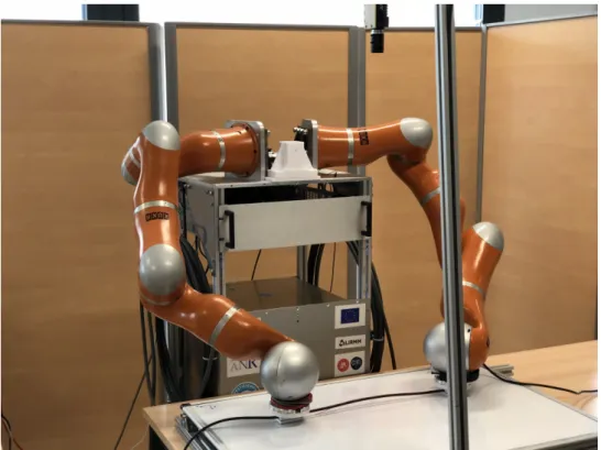
We use the BAZAR robot [Cherubini et al., 2019] equipped with two lightweight KUKA LWR IV robots for the dual arm setup (see Fig. 4.6).
We design two grippers to ensure the manipulation of the cable without slipping (see Fig. 4.5). In the left figure, the blue gear is attached to the robot. The black cylinder represents the cable, and the yellow gear fastens the cable rigidly.
(a) Cable gripper mechanical design. (b) Cable gripper mounted on the robot.
Figure 4.5: The cable gripper.
The cable is gripped by two end-effectors. An Allied Visionr AVT camera is placed
perpendicular to the manipulation plane to track the shape of the cable during manip-ulation. The image resolution is 1936 × 1456. A Linux-based 64-bits PC processes the image at a frame rate of 33.3Hz.
The overall hardware setup is showed in Fig. 4.6.
To test the robustness of the algorithm, we prepare two cables with different thick-nesses. The diameter of the thin cable is 5.88 millimeters, and the thick cable is 7.66 millimeters. Under the same inputs from the robot, the two cables result in slightly different shapes.