Ventilation performance measurement of a decentralized mechanical system with heat recovery using tracer gas decay method

Ventilation performance measurement of a decentralized mechanical

system with heat recovery using Tracer gas decay method

Youness Ajaji1,*, Philippe André1 1

University of Liege, Arlon Campus Environnement, Arlon Belgium *

Corresponding email: youness.ajaji@ulg.ac.be

SUMMARY

In decentralized mechanical ventilation, air supply being very close to exhaust, short-circuiting of the supply air towards the extraction point may occur, increasing energy consumption of the system and decreasing air diffusion quality. To estimate this quality together with thermal comfort, we measured in a climatic chamber effectiveness of a local ventilation prototype using tracer gas decay method, as well as air velocity.

The results show that air change efficiencies, are higher than 0.5 for 50%, 80%, 100% ventilation regimes, and fluctuate between 0.41 and 0.43 for 20% one. Local air change indexes are higher than 1 for regimes higher than 50%, and lower than 0.89 for 20% one. All measured velocities are lower than 0.08m/s. We conclude that the prototype achieves an acceptable air diffusion quality for nominal ventilation regime. But it is not acceptable under 20%. Measurements of velocities do not show any thermal discomfort.

KEYWORDS

Air change efficiency, local air change index, thermal comfort, mixing ventilation.

1 INTRODUCTION

Because of the need to reduce the use of energy, since the mid-1970s and because the energy consumption for maintaining an acceptable environment in buildings constitutes the largest part of the total energy demand in developed countries, several measures have been taken by governments, groups and individuals to reduce the usage of energy for heating and cooling buildings (Awbi, 2003). That’s why insulation and tightness of envelope buildings became better. The improvement of envelope buildings tightness means a strong decrease of natural infiltrations/exfiltrations which contribute to air change of indoor environment, and the necessity of using additional ventilation to bring fresh air to the occupant. The main advantages of decentralized mechanical systems compared to centralized ones are flexibility as they provide ventilation on demand in each room ensuring a maximum effectiveness and a minimum of energy waste (Aparecida Silva et al. 2011), and ergonomics as they are simply installed on an exterior wall or a window frame. Thus they are preferred in residential buildings under renovation. Air supply being very close to exhaust, short-circuiting of the supply air towards the extraction point may occur, decreasing air diffusion quality and increasing energy consumption of the system.

To estimate this quality together with thermal comfort, we measured in a climatic chamber effectiveness of a local ventilation prototype using CO2 tracer gas decay method, as well as air velocity. We evaluated air change efficiency and local air change index – assuming isothermal jets – for 4 ventilation regimes and 6 locations within the occupied zone, and we measured velocity at these locations. The local air change index is defined by ASHRAE Standard 62 (Koffi, 2009). Before starting these measurements, we measured infiltrations through the laboratory climatic chamber envelope using a blower door test according to the standard EN

ISO 13829 (2001) and compared the results with those obtained with CO2 gas tracer decay method. The coherence of the results justifies the choice of CO2 as tracer gas.

2 CONCEPTS OF VENTILATION EFFICIENCY Air mixing quality

It depends on many parameters (AIVC, 1996): scale of turbulence, distribution and size of infiltration paths, diffuser characteristics, inlet air velocity and supply rate... This air mixing quality can be evaluated by global and local air renewal effectiveness indexes. The global index measures air renewal effectiveness in the whole room while the local index evaluates air renewal effectiveness in an arbitrary location within the occupied zone.

The nominal time constant is given by the inverse of the specific flow. This is the minimum

time possible it takes for air, once entering a room to be completely replaced.

The local mean age of air ԎL at an arbitrary location p in a room is the average time it takes

for air, once entering a room to reach the location p. If the pollutant is injected inside the room once (single injection) then:

0 ( ) (0) L p C t dt C

 

_

The room mean age of air is the average of the local mean ages for all points of the room. If

the injection of pollutant is unique then:

0 0 ( ) ( ) e m e t C t dt C t dt     





Where Ce is the concentration of pollutant at the exhaust at time t.

The air change time Ԏr is the time it takes for air, once entering a room, to be completely

replaced. It is equal to twice the room mean age of air.

Air change efficiency εm is the ratio between the nominal time constant and the air change

time: 2 n n m r m        (Koffi, 2009)

As the minimum possible value of air change time is equal to the nominal time constant, then this index is lower than 1 or equal. For a piston ventilation, as there is no mixing between outdoor air and indoor air, the indoor air is completely replaced in a time equal to the nominal time constant: εm=1. For a perfect mixing ventilation half of the indoor air is replaced in a time equal to the nominal time constant: εm=0.5. Between these two ideal configurations if 0.5<εm<1 then the effectiveness is good. If εm<0.5 then the ventilation system is not effective.

The local air change index measures the air exchange at a location p within the occupied

zone because in most cases air exchange is not uniform within the room. 2 n L L      (Koffi, 2009) 3 MATERIALS/METHODS

We measured the ventilation efficiency of a local ventilation device using decay method and CO2 as tracer gas. The measurements were done in the laboratory climatic chamber at Arlon Campus Environment (figure 1). We performed all tests under isothermal conditions. We measured air temperatures in the climatic room and the buffer zone, and supply air temperatures using thermocouples. The measurement accuracy is 0.1K. During tests, the sliding door (figure 1) was open so that the buffer zone is not polluted by the CO2 removed

from exhaust of the ventilation. We measured CO2 concentrations at six locations within the occupied zone using two CO2 infrared sensors placed at 1.5m above the ground and a third one at the exhaust (figure 1). The CO2 infrared sensors are made for HVAC applications. Their accuracy is 50ppm +2% read value. The measurement range is [0; 2000ppm]. Thus tests were done at different time but at very similar temperature conditions. After placing two CO2 infrared sensors in the occupied zone and a third one at the ventilation exhaust, we turned on the mixing fan in the climatic chamber and we injected CO2 into the room until the concentration reached a sufficient value. The mixer turned on for 25min. Thus a uniform initial concentration could be achieved in the whole chamber. Then we turned off the mixer and we turned on the local ventilation. 4 regimes were tested as explained in the introduction. All sensors are connected to a data analyser and data are recorded every minute. We also measured air velocities at same locations as CO2 concentrations were measured, using three omnidirectional hot wire anemometers. Their accuracy is 3% and the measurement range is [0.08; 5m/s].

Figure 1. a) Plan of BEMS’ (Building Energy Monitoring and Simulation) laboratory ground floor at Arlon Campus Environment. The climatic chamber is surrounded by a buffer zone where thermal environment is controlled, b) CO2 sensors disposition within the occupied zone of the climatic chamber. The local ventilation prototype is placed 2m above the ground. We assess ventilation exhaust and supply air flow rates measuring differential pressures by using pressure capacitive sensors. The local ventilation prototype tested is under an exploded form i.e. the supply and exhaust fans are not put in the ventilation box but in two air boxes connected to the ventilation box by two pipes. To evaluate the flow rates we use two nozzles put upstream the supply fan and downstream the exhaust fan. Each nozzle is connected to an air box in which the pressure is constant and to the buffer zone air. The capacitive pressure sensors accuracy is 1% and the measurement range is [0; 500Pa]. They are used for HVAC applications.

4 RESULTS

We describe the results measured at each of the six locations. The x-axis unit is the second. The y-axis unit is the ppm. All results were calculated as concentration of CO2 over concentration of initial fresh air.

1a 1a 1a 1a

Figure 2: CO2 concentration at locations 1a and 1b after a unique injection of CO2. The grey curve is a trend one. From left to right: ventilation regimes 100, 80, 50 and 20%.

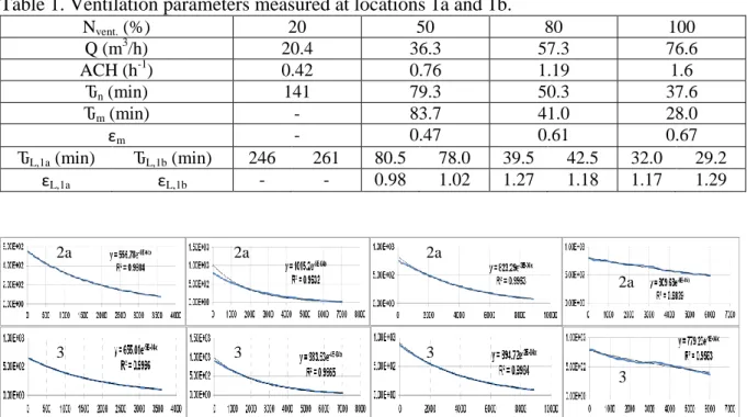
Table 1. Ventilation parameters measured at locations 1a and 1b.

Nvent. (%) 20 50 80 100 Q (m3/h) 20.4 36.3 57.3 76.6 ACH (h-1) 0.42 0.76 1.19 1.6 Ԏn (min) 141 79.3 50.3 37.6 Ԏm (min) - 83.7 41.0 28.0 εm - 0.47 0.61 0.67

ԎL,1a (min) ԎL,1b (min) 246 261 80.5 78.0 39.5 42.5 32.0 29.2

εL,1a εL,1b - - 0.98 1.02 1.27 1.18 1.17 1.29

Figure 3: CO2 concentration at locations 2a and 3 after a unique injection of CO2. The grey curve is a trend one. From left to right: ventilation regimes 100, 80, 50 and 20%.

Table 2. Ventilation parameters measured at locations 2a and 3.

Nvent. (%) 20 50 80 100 Q (m3/h) 20.2 36.2 57.2 76.6 ACH (h-1) 0.42 0.75 1.19 1.6 Ԏn (min) 142.9 79.6 50.3 37.6 Ԏm (min) 164.5 55.6 34.6 32.6 εm 0.43 0.72 0.73 0.58

ԎL,2a (min) ԎL,3 (min) 210 161 68.5 76.5 39.2 44.5 33.1 33.7

εL,2a εL,3 0.68 0.89 1.16 1.04 1.28 1.13 1.14 1.16 1b 1b 1b 1b 2a 2a 2a 2a 3 3 3 3 4 4 4 4 2b 2b 2b 2b

Figure 4: CO2 concentration at locations 4 and 2b after a unique injection of CO2. The grey curve is a trend one. From left to right: ventilation regimes 100, 80, 50 and 20%.

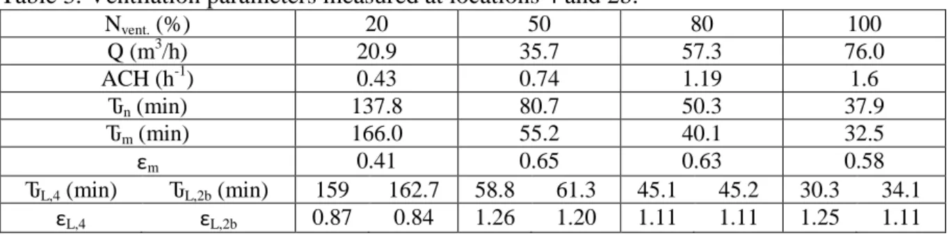
Table 3. Ventilation parameters measured at locations 4 and 2b.

Nvent. (%) 20 50 80 100 Q (m3/h) 20.9 35.7 57.3 76.0 ACH (h-1) 0.43 0.74 1.19 1.6 Ԏn (min) 137.8 80.7 50.3 37.9 Ԏm (min) 166.0 55.2 40.1 32.5 εm 0.41 0.65 0.63 0.58 ԎL,4 (min) ԎL,2b (min) 159 162.7 58.8 61.3 45.1 45.2 30.3 34.1 εL,4 εL,2b 0.87 0.84 1.26 1.20 1.11 1.11 1.25 1.11

During all tests air velocities measured were less than 0.08m/s.

5 DISCUSSION

We note that the temperature differences between the climatic chamber and the buffer zone ΔT are low. The average temperature differences during all the tests is 0.8K. So we can consider that all the tests were performed under isothermal conditions. According to climatic chamber air permeability measurements that we had performed using the fan pressurization method done according to the standard EN ISO 13829 (2001), Q4pa=0.4m3/h/m2 under ΔT=5k. This airtightness corresponds to that of a new building in Luxembourg. However during effectiveness ventilation measurements, ΔT is much lower so the stack effect is also much lower. Therefore we neglect infiltrations. We note that the decay of tracer gas concentration is exponential in accordance with the assumptions. The lowest value of the determination factor

R2 for testing regimes 50, 80, 100% is 0.9632 (figure 3). The highest one is 0.9997 (figure 2). At 20% regime the lowest value recorded is 0.7299 for the test performed at the location 1a and 0.936 for the test performed at the location 1b (figure 2). For both these tests, we measured an air change efficiency higher than 1. The reason of this inconsistency is that the room mean ages of air at these two locations are very low: 80min (table 1). This value is close to those measured for 50% regime. Therefore we do not take into account these two results in our conclusions. All other results for the remaining 22 tests are consistent. The figures 2, 3, 4 show that the decay rates increase with the ventilation regime. We note that mean and local ages decrease with the ventilation regime. On the other hand, local ages are relatively independent of the measuring locations within the occupied zone. This is typical of a mixing ventilation.

Morel and Gnansounou (2008) said that in general, draughts are avoided if air velocities do not exceed 0.2m/s in the occupied zone. It is even recommended not to exceed 0.1m/s. In our case, no discomfort can be felt whatever the ventilation regime is, since all the velocities measured at 1.5m above the ground within the occupied zone are less than 0.08m/s.

The measured air change efficiencies fluctuate from 0.58 to 0.73 (tables 1, 2, 3) for most measurements at 50, 80 and 100% ventilation regimes. This means that mixing of fresh air and polluted air is well achieved and the ventilation is effective. For the nominal regime we measured 0.47 for the first two tests (table 1). The air mixture is close to the perfect one. At 50, 80, 100% regimes and at the locations 2a, 2b, 3, 4, we measured local air change indexes fluctuating from 1.04 to 1.28 (tables 2 and 3). Therefore air is well mixed. At 50% regime at locations 1a and 1b local indexes vary from 0.98 to 1.02 (table 1). The air mixture is nearly perfect. At 20% regime air change efficiencies during all tests fluctuate between 0.41 and 0.43

(tables 2 and 3): the ventilation is not effective. At 20% regime, we find local air change indexes lower than 1: between 0.68 and 0.89 (tables 2 and 3). This confirms that the ventilation is not effective, but it could be improved:

1. Naturally because room occupancy will contribute to increase the intensity of turbulence, thus improving the mixing of air.

2. By increasing the average inlet air velocity as air velocities within the occupied zone are low, reducing the free area of the diffuser (this is the sum of the smallest areas of the openings of an air terminal device through which air can pass (Awbi, 2003)). Thus turbulence is also increased.

6 CONCLUSIONS

We conclude that the local ventilation prototype achieves an acceptable air diffusion quality for nominal ventilation regime (or higher). So the proximity of the exhaust from the supply does not prevent the ventilation from being effective. Measurements of velocities do not show any thermal discomfort. For 20% regime the air diffusion quality can be easily improved as explained in the end of the discussion.

We performed all measurements under isothermal conditions. The temperature difference between the air jet and the room air creates buoyancy forces which influence jet behaviour. In winter conditions this temperature difference can be 5K or more, depending on the air-air exchanger efficiency. The significance of buoyancy depends on the ratio between buoyancy forces and inertia forces due to jet momentum (Yue, 2001; Awbi, 2003). Therefore the next step will consist of measuring thermal comfort for non isothermal jets and we will also simulate a cold wall, a heater and occupancy.

ACKNOWLEDGEMENT

The support of the Walloon Region for funding this research which is a part of the project called GREEN+, in the framework of the “Marshall Plan” is gratefully acknowledged.

7 REFERENCES

AIVC. 1996. A Guide to Energy Efficient Ventilation. Air Infiltration and Ventilation Centre, University of Warwick (Great Britain), 274 pages.

Aparecida Silva C, Gendebien S, Hannay J, Hansens N, Lebrun J, Lengele M, Masy G. and Prieels L. 2011. Decentralized mechanical ventilation with heat recovery. In

Proceedings of the 32nd AIVC Conference and 1st TightVent Conference on Optimal Airtightness Performance – Brussels, pp. 26-31.

Awbi H. B. 2003. Ventilation of Buildings. USA and Canada: Spon Press, 522 pages. Fracastero G.V, Di Tommaso R.M, and Nino E. 2000. Correlation of air change efficiency

with Archimedes Number in a ventilated test room, Roomvent 2000 – System Efficiency. Koffi J. 2009. Multi-criteria analysis of ventilation strategies used in single family houses.

Ph.D. Thesis, University of La Rochelle (France), 224 pages.

Morel N. and Gnansounou E. 2008. Energétique du bâtiment. Swiss Federal Institute of Technology of Lausanne (Switzerland), 223 pages.

Muhic S. and Butala V. 2006. Effectiveness of personal ventilation system using relative decrease of tracer gas in the first minute parameter, Energy and Buildings 38 (2006) 534 – 542.

NF EN 13829. 2001. Thermal performance of buildings – Determination of air permeability of buildings – Fan pressurization method.

Yue Z. 2001. Air jets in ventilation applications. Ph.D. Thesis, Royal Institute of Technology (Sweden), 151 pages.