Unveiling the β Pictoris system, coupling high contrast imaging,
interferometric, and radial velocity data
A. M. Lagrange
1,2,3, P. Rubini
4, M. Nowak
5, S. Lacour
2, A. Grandjean
1, A. Boccaletti
2, M. Langlois
6,
P. Delorme
1, R. Gratton
7, J. Wang
8, O. Flasseur
1, R. Galicher
2, Q. Kral
2, N. Meunier
1, H. Beust
1, C. Babusiaux
1,9,
H. Le Coroller
10, P. Thebault
2, P. Kervella
2, A. Zurlo
10,11, A.-L. Maire
12,13, Z. Wahhaj
14, A. Amorim
15,16,
R. Asensio-Torres
13, M. Benisty
1, J. P. Berger
1, M. Bonnefoy
1, W. Brandner
13, F. Cantalloube
13, B. Charnay
2,
G. Chauvin
1,17, E. Choquet
10, Y. Clénet
2, V. Christiaens
18, V. Coudé du Foresto
2, P. T. de Zeeuw
19,20, S. Desidera
7,
G. Duvert
1, A. Eckart
21,22, F. Eisenhauer
20, F. Galland
1, F. Gao
20, P. Garcia
16,23, R. Garcia Lopez
24,13, E. Gendron
2,
R. Genzel
20, S. Gillessen
20, J. Girard
25, J. Hagelberg
26, X. Haubois
14, T. Henning
13, G. Heissel
2, S. Hippler
13,
M. Horrobin
21, M. Janson
13,27, J. Kammerer
28,29, M. Kenworthy
19, M. Keppler
13, L. Kreidberg
13,30, V. Lapeyrère
2,
J.-B. Le Bouquin
1, P. Léna
2, A. Mérand
28, S. Messina
31, P. Mollière
13, J. D. Monnier
32, T. Ott
20, G. Otten
10,
T. Paumard
2, C. Paladini
14, K. Perraut
1, G. Perrin
2, L. Pueyo
25, O. Pfuhl
28, L. Rodet
33, G. Rodriguez-Coira
2,
G. Rousset
2, M. Samland
13, J. Shangguan
20, T. Schmidt
34, O. Straub
20, C. Straubmeier
21, T. Stolker
35,
A. Vigan
10, F. Vincent
2, F. Widmann
20, J. Woillez
28, and the GRAVITY Collaboration
(Affiliations can be found after the references) Received 2 July 2020 / Accepted 21 August 2020
ABSTRACT
Context. The nearby and young β Pictoris system hosts a well resolved disk, a directly imaged massive giant planet orbiting at '9 au, as well as an inner planet orbiting at '2.7 au, which was recently detected through radial velocity (RV). As such, it offers several unique opportunities for detailed studies of planetary system formation and early evolution.
Aims. We aim to further constrain the orbital and physical properties of β Pictoris b and c using a combination of high contrast imaging, long base-line interferometry, and RV data. We also predict the closest approaches or the transit times of both planets, and we constrain the presence of additional planets in the system.
Methods. We obtained six additional epochs of SPHERE data, six additional epochs of GRAVITY data, and five additional epochs of RV data. We combined these various types of data in a single Markov-chain Monte Carlo analysis to constrain the orbital parameters and masses of the two planets simultaneously. The analysis takes into account the gravitational influence of both planets on the star and hence their relative astrometry. Secondly, we used the RV and high contrast imaging data to derive the probabilities of presence of additional planets throughout the disk, and we tested the impact of absolute astrometry.
Results. The orbital properties of both planets are constrained with a semi-major axis of 9.8 ± 0.4 au and 2.7 ± 0.02 au for b and c, respectively, and eccentricities of 0.09 ± 0.1 and 0.27 ± 0.07, assuming the HIPPARCOSdistance. We note that despite these low fitting error bars, the eccentricity of β Pictoris c might still be over-estimated. If no prior is provided on the mass of β Pictoris b, we obtain a very low value that is inconsistent with what is derived from brightness-mass models. When we set an evolutionary model motivated prior to the mass of β Pictoris b, we find a solution in the 10–11 MJuprange. Conversely, β Pictoris c’s mass is well
constrained, at 7.8 ± 0.4 MJup, assuming both planets are on coplanar orbits. These values depend on the assumptions on the distance of
the β Pictoris system. The absolute astrometry HIPPARCOS-Gaia data are consistent with the solutions presented here at the 2σ level, but these solutions are fully driven by the relative astrometry plus RV data. Finally, we derive unprecedented limits on the presence of additional planets in the disk. We can now exclude the presence of planets that are more massive than about 2.5 MJupcloser than 3 au,
and more massive than 3.5 MJupbetween 3 and 7.5 au. Beyond 7.5 au, we exclude the presence of planets that are more massive than
1–2 MJup.
Conclusions. Combining relative astrometry and RVs allows one to precisely constrain the orbital parameters of both planets and to give lower limits to potential additional planets throughout the disk. The mass of β Pictoris c is also well constrained, while additional RV data with appropriate observing strategies are required to properly constrain the mass of β Pictoris b.
Key words. techniques: high angular resolution – techniques: radial velocities – planets and satellites: detection – planets and satellites: fundamental parameters
1. Introduction
The nearby (parallax = 51.44 ± 0.12 mas,van Leeuwen 2007)1 β Pictoris system has been intensively studied since the mid 1980s, when a circumstellar debris disk of dust was first
1 GaiaDR2 provides a parallax of 50.62 ± 0.12 mas. We note that the
Gaiaparallax is at 2.3 σ from the HIPPARCOSone within the provided
imaged (see Smith & Terrile 1984, for the discovery image). Evaporating exocomets were discovered (Kiefer et al. 2014, and references there-in) soon afterwards. While both the disk shape
uncertainties but we know that those are underestimated and that sys-tematics are to be taken into account (e.g.,Arenou et al. 2018) which reconciles the two values.
A18, page 1 of17
and the infalling comets were attributed to planets in the 1990s, it took more than a decade to detect the first planet in the system (Lagrange et al. 2010). It appeared that β Pictoris b could indeed explain both the disk inner warp (Augereau et al. 2001) and the infalling comets, provided it had a nonzero eccentricity (Beust & Morbidelli 1996,2000). Many high contrast imaging (hereafter HCI) observations have constrained its orbital properties, and, in particular, excluded highly eccentric (e ≥ 0.25) orbits (Lagrange et al. 2019a). Using just one observation with the GRAVITY long baseline interferometer of the position of β Pictoris b relative to the star combined with previously published GPI (Macintosh et al. 2008) HCI data, GRAVITY Collaboration (2020) found an eccentricity of 0.11–0.20, whileNielsen et al.(2020), using newly re-calibrated GPI data found an eccentricity in the range of 0.09–0.16. However, the lower limits on β Pictoris b’s eccentricity remained quite elusive. Finally, using the K-STacker algorithm, which is an approach that is fully different from the Markov-chain Monte Carlo (MCMC) based methods,
Le Coroller et al.(2020) derived an eccentricity of 0.07. β Pictoris b is the only directly imaged exoplanet with a con-strained dynamical mass. Radial velocity (RV) data showed that, assuming a zero eccentricity, the planet mass should not exceed 15 MJup(Lagrange et al. 2012). A first order combined analy-sis of HCI and RV data (Bonnefoy et al. 2014) led to a similar result. This was also in agreement with brightness-mass rela-tionships, which gave values between 9 and 13 MJup(Lagrange
et al. 2010). Using HIPPARCOSand Gaia data,Snellen & Brown
(2018) derived a mass in the range of [10,12] MJup. Also, based on the GPI relative astrometry and an analysis of HIPPARCOS -Gaia data, Kervella et al. (2019) find a mass of 13.7+6
−5 MJup.
Nielsen et al.(2020), using mainly NACO, GPI relative astrom-etry up to November 2018 (using a new calibration of GPI data), as well as HIPPARCOSand Gaia absolute astrometry, find a mass of 12.8+5.3−3.8MJup. Taking into account HIPPARCOSand Gaia data also increases the semi major axis (sma) of β Pictoris b’s orbit to 10.2 au, while they obtain an sma of 9.3 au when they do not take the HIPPARCOSand Gaia data into account. Using NACO, GPI prior to 2017, as well as long base line GRAVITY inter-ferometric data, GRAVITY Collaboration (2020) find a mass of 12.7 ± 2.2 MJup; the range of these values is just compatible with the modeling of the Gravity K-band spectrum. All of these estimates that consider only one planet need to be revised as a recent analysis of ESO/HARPS high resolution spectroscopic data obtained since the beginning of the instrument (2003–2018) has led to the discovery of a second, inner planet (Lagrange et al. 2019a), with a mass of '9 times the mass of Jupiter, orbiting at '2.7 au on a slightly eccentric (e ' 0.2) orbit. Taking β Pictoris c into account,Dupuy et al.(2019) derived a mass for β Pictoris b in the range of [10,16] MJup, whileNielsen et al.(2020) find a mass of 8.35 MJup, which is much lower than that found without the RV data. Nonetheless, the use of the absolute astrometric data remains tricky at this stage because of the still limited information provided by Gaia DR2 and the fact that this star is saturated in the observations of Gaia. This aspect is addressed in detail inNowak et al.(2020).
Improving the planets orbit and mass characterization requires both very precise relative astrometry, hopefully on both planets, on a time basis as long as possible, as provided by GRAVITY (see GRAVITY Collaboration 2020, in the case of β Pictoris b), and long time series RV data. In this paper, we present new SPHERE, GRAVITY, and HARPS observations of β Pictoris . We use these new and previous data to combine, in a single MCMC analysis, HCI, RV, and GRAVITY data on β Pictoris b to further constrain both planets.
The system may also host additional planets. The presence of clumps seen at mid-IR (Telesco et al. 2005;Okamoto et al. 2004;
Wahhaj et al. 2003) and asymmetries seen in sub-mm (ALMA) data (seeCataldi et al. 2018, and ref. there-in) as well as the pres-ence of the innermost hole (Lagage & Pantin 1994) indicate that planets could be present in the disk. InLagrange et al.(2019b), we estimated the probability of presence of additional planets from a fraction of an au up to hundreds of au, coupling HCI NACO data with RV data. Companions with masses larger than 15 MJupwere excluded throughout the disk except between 3 and 5 au with a 90% probability. We could, moreover, exclude the presence of planets that are more massive than 3 MJupcloser than 1 au and further than 10 au, with a 90% probability. In the 3–5 au region, we excluded companions with masses larger than 18 (resp. 30) MJupwith probabilities of 60 (resp. 90)%. The present set of data, combined with the results of the properties of β Pictoris b and c, allows a significant improvement in the mass upper limits of possible additional planets.
The various data are described in Sect.2. The orbital analy-sis is performed in Sect.3and some consequences are discussed in Sect.4. We combined all HCI (more than 30 epochs) and all RV data to revisit the probability of detection of additional plan-ets in Sect.5. The conclusion and perspectives are presented in Sect.6.
2. Observations and data 2.1. SPHERE data
Six new high contrast, IRDIS (Dohlen et al. 2008;Vigan et al. 2010) and IFS (Claudi et al. 2008; Zurlo et al. 2014) coro-nagraphic SPHERE (Beuzit et al. 2019) data were obtained between October 2018 and February 2020. The first three datasets were taken as part of the SPHERE SHINE GTO (Desidera et al, in prep.), and the last three as part of a clas-sical program (PI Lagrange; 0104.C-0418(D), 0104.C-0418(E), 0104.C-0418(F)). The October 2018 data immediately followed the first observations (in Sept. 2018) of β Pictoris b after its clos-est approach to the star described inLagrange et al.(2019a). All but one of the new datasets presented here were obtained in the H2 (central wavelength = 1.59 µm; width = 0.055 µm) and H3 (central wavelength = 1.67 µm; width = 0.056 µm) IRDIS nar-row bands, as well as in YJ (0.95â1.35 µm, spectral resolution R '54) with IFS. One data set (March 2019) was taken in the K1 (central wavelength = 2.1025 µm ; width = 0.102 µm) and K2 (central wavelength = 2.255 µm ; width = 0.109 µm) IRDIS nar-row bands, and in YH (0.95â1.65 µm, R ' 33) with IFS. All data were taken with apodized Lyot coronagraphs, including either a 185 mas focal mask (N_ALC_Y JH_S ) or a smaller (145 mas) mask (N_ALC_Y J_S ), when the planet was closer to the star, as well as a pupil mask. Our new data were recorded in stabi-lized pupil mode so as to perform angular differential imaging (ADI) post-processing (Marois et al. 2006;Galicher et al. 2018), and with the waffle mode on. This mode allows one to apply voltages on the deformable mirror to generate four symmetrical spots in the form of a “cross” or a “plus” shape; these spots are used to measure the star position at the center of the pattern.
Each observing sequence followed the usual following steps: PSF–Coronographic observations–PSF–Sky. The PSF were used as relative photometric references and to obtain an estimate of the PSF just before and just after the observations. This PSF was used to model the planet signal during the characterization step. Sky data were recorded at the end of the coronagraphic sequence to get an estimate of the background level in the science
2018-10-17 IRDIFS 2 × 30 × 54 1.12 54.5 1.03 3.2 47tuc −1.804 ± 0.045 12.248 ± 0.009 2018-12-14 IRDIFS 2 × 30 × 32 1.12 33.3 0.47 5.8 47tuc −1.764 ± 0.021 12.248 ± 0.005 2019-03-10 IRDIFS 12 × 19 × 16 1.12 32.1 0.71 5.4 ngc3603 1.764 ± 0.065 12.255 ± 0.015 2019-11-02 IRDIFS 3 × 23 × 32 1.12 32.2 0.87 3.4 ngc3603 −1.773 ± 0.065 12.248 ± 0.005 2019-12-21 IRDIFS 4 × 17 × 30 1.13 30.6 0.65 7.6 47tuc −1.771 ± 0.081 12.245 ± 0.017 2020-02-07 IRDIFS 4 × 17 × 32 1.12 30.7 0.60 5.1 47tuc −1.771 ± 0.081 12.245 ± 0.017 2018-09-22 GRAVITY-MED 30 × 10 × 17 1.19 52 0.77 6.7 2019-09-12 GRAVITY-MED 10 × 32 × 3 1.9 4.3 1.6 1.2 2019-11-09 GRAVITY-HIGH 100 × 8 × 5 1.44 21.4 0.78 5.4 2019-11-11 GRAVITY-HIGH 100 × 8 × 5 1.17 33.7 0.79 3.4 2020-01-07 GRAVITY-HIGH 100 × 8 × 6 1.25 32.1 1.65 1.7 2020-01-07 GRAVITY-MED 10 × 32 × 3 1.16 8.8 2.84 1.2 2020-02-09 GRAVITY-MED 10 × 32 × 2 1.26 21 0.74 13.4
Notes. DIT × NDIT × Nexp refers to the IRDIS observations. AM stands for the mean airmass, ∆par for the variation of the parallactic angle during the coronagraphic sequence, TN for true north, and Scale for Plate Scale. The seeing and coherence time are mean values along the coronographic sequence. Plate scales and TN were measured on noncoronagraphic data.
images. Finally, the pixel scales and true north were measured from IRDIS observations of astrometric fields (see Table1). We note that in the March 2019 set of data, the IRDIS data were sat-urated very close to the mask, so only the IFS are considered hereafter for this set.
The IRDIS and IFS data were reduced as described in
Chauvin et al.(2017) andDelorme et al.(2017), and using the SPECAL tool developed for SPHERE (Galicher et al. 2018). For each epoch, all individual data frames were recentered using the waffles to create a single cube, which was then analyzed to remove the stellar halo and measure the astrometry of the planet. In the IRDIS data, the β Pictoris b positions relative to the star and associated uncertainties of the PCA images were mea-sured in two ways: (1) fitting a model of the planet to the detected source, and (2) injecting a negative planet into the initial data cube and processing it to minimize the local flux in the ADI-processed data. These two approaches are described in Sect. 3 of
Galicher et al.(2018). They both use the PSF recorded prior to and after the coronagraphic data.
In the IFS data, the positions of β Pictoris b were also mea-sured in two ways: (1) with PCA, as described in Zurlo et al.
(2016), and (2) using the PACO software (Flasseur et al. 2020). The astrometric uncertainties were estimated using the errors associated with these fits as well as star centering errors and the errors on the pixel scales and true north.
With these new data, relative astrometric values at 18 epochs are now available. Figure1shows the positions obtained with the various methods. The astrometric measurements derived from method 1 and method 2 for IRDIS are in good agreement. In the following, we consider the average of these two values. TableC.1 provides the measurements of β Pictoris b’s position in the IRDIS data (average of methods 1 and 2) as well as the previous NACO astrometric data used in the present study. The astrometric measurements on IFS data derived from method 1 and method 2 significantly differ, and the values found with IFS method 1 are closer to those found on IRDIS than those found with IFS method 2. This certainly illustrates that the PCA and PACO methods are intrinsically different, and they do not share the same biases. In the following, we use the values of
β Pictoris b’s position found with method 1 in the IFS data. They are provided in TableC.1.
2.2. GRAVITY data
Six new pieces of high accuracy astrometric data were obtained with the GRAVITY instrument (GRAVITY Collaboration 2017) in the K band. The first astrometric measurement is an updated value of the astrometry published byGRAVITY Collaboration
(2020). Most of the other observations were obtained in the context of the ExoGRAVITY large program (PI: S. Lacour; 1104.C-0651), which is an interferometric survey of the dynam-ics and chemical composition of directly imaged exoplanets. An extra data point was taken as backup for the NGC1068 observa-tions (PI: O. Pfuhl, 0104.B-0649). The log of the observaobserva-tions are presented in Table 1. Three of the observations were per-formed in medium resolution (R = 500), two in high resolution (R = 4000); and during one night (7 Jan 2020), the observations were taken with both modes.
The observation sequence was the same as in GRAVITY Collaboration(2019): the fringe tracker (Lacour et al. 2019) uses the central star to correct the atmospheric piston, but also to serve as a reference for the astrometry. The science fiber feed-ing the spectrometer points, alternatively, between the position of the star and the position of the planet. While the star can be seen on the acquisition camera, the position of the planet was obtained from dedicated software based on GPI data, which is available to the community2, or by our estimations when using SPHERE data as input for the orbit estimation.
The reduction starts by using the official GRAVITY pipeline (Lapeyrere 2014) to reduce the images to uncalibrated visibili-ties. The complex visibilities are then all phased with respect to the fringe tracker phase. From this point on, we used our tools to fit the phase and the spectra of the coherent flux3. The inter-ferometric baselines, which are the equivalent of the imaging plate-scale (Woillez & Lacour 2013), use the Earth orientation
2 www.whereistheplanet.com
200 100 0 100 200 RA (mas) 400 300 200 100 0 100 200 300 DEC (mas) NACO IFS-PACO IFS IRDIS-1 IRDIS-2 GRAVITY 60 80 100 120 140 160 RA (mas) 120 140 160 180 200 220 240 260 280 DEC (mas) NE NACOIFS-PACO IFS IRDIS-1 IRDIS-2 GRAVITY 200 180 160 140 120 100 80 60 40 RA (mas) 300 250 200 150 100 DEC (mas) SW NACOIFS-PACO IFS IRDIS-1 IRDIS-2 GRAVITY
Fig. 1.Relative astrometry of β Pictoris b obtained with the various analysis methods (left). We also plotted the astrometric positions measured by
NACO in the full FoV. Zooms on the NE and SW quadrants focusing on SPHERE points (middle and right).
parameters (EOP) to find the position of the telescopes with respect to the sky. The results of the astrometric fits are pre-sented in TableC.2. The accuracy, presented as σ∆RAand σ∆Dec, is on the order of 100 µas. However, the geometry of the inter-ferometer has a profound impact on the error bars. Because the baselines are considerably longer in the north-east direction, that is, 130 m compared to 50 m, the error bars are consistently worse in the north-west direction. This characteristic is accounted for by using the correlation coefficient ρ. This parameter varies between −1 for an anticorrelation, to 1 for a total positive cor-relation, and zero for no correlation. The correlation coefficients are given in TableC.2, and they are typically between −0.2 and −0.8. They are used in the MCMC analysis.
2.3. HARPS data
More than 1900 new HARPS spectra were obtained at five differ-ent epochs since the β Pictoris c discovery paper (Lagrange et al. 2019a) under programs 098.C-0739(A) and 0104.C-0418(A) (PI Lagrange). At each epoch, long sequences of data (several hours per night over 1, 3, 3, 4, and 3 days, respectively) were recorded to allow for the proper extraction of the planet signal. Indeed, the star is a high frequency (about 23–30 min) and high ampli-tude (up to 2 km s−1) pulsator, and the stellar pulsations need to be subtracted from the signal. The RVs were measured as in our previous works, using our SAFIR tool (Galland et al. 2005) and using the same approach as inLagrange et al.(2019a). Basically, for each spectrum, the RV is computed, in the Fourier plane, with respect to a reference spectrum made of an average of all available and suitable data.
To estimate the stellar pulsations, we used Method 2 described in detail inLagrange et al.(2019a), which consists in fitting the data with one sine function plus an offset, computing the residuals, repeating the process on the residuals, and so on, nine times. The final offset represents the planets-induced RV plus a constant offset due to the fact that the RVs are relative to a reference spectrum. We refer the readers toLagrange et al.
(2019a) for detailed explanations. The offset values determined for the new epochs as well as previous ones are provided in Table C.3. We note that the offsets presented here, similar to most of those recorded since JDB-2 454 000 = 4000, have low
uncertainties. This is because we have significantly increased the duration of the visits (several hours per night and for three or more consecutive nights). The fits are provided in AppendixA.
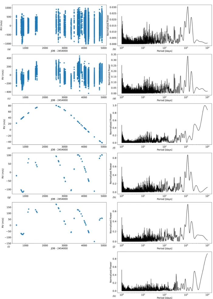
Figure2 shows the RV time series (7000 data points since 2003) before and after correction from the pulsation signals. Since the last data were published in Lagrange et al.(2019a), the RV have increased again due to β Pictoris c.
The periodograms associated with both the raw and pulsa-tion data show a peak at about 1200 d, which is not present in the window function, due to β Pictoris c. We conclude that the additional data presented in this paper confirm the presence of β Pictoris c.
3. Properties of β Pictoris b and c
The aim of the present paper is to combine various types of observational data into a single analysis. We used a Markov-chain Monte Carlo (MCMC) Bayesian analysis to derive the probabilistic distribution of orbital and physical solutions. The code is an upgrade of the one presented in Grandjean et al.
(2019); it uses the affine invariant MCMC ensemble sampler emcee (Foreman-Mackey et al. 2013). The model includes the orbital parameters of β Pictoris b and c as well as the mass and distance of β Pictoris . Walker moves were selected using differ-ential evolution (80% DEMove + 20% DESnookerMove); these move rules ensure that steps taken by walkers are automatically scaled according to the current parameter distributions.
We first used only the astrometry deduced from the NACO + SPHERE HCI data on β Pictoris b, then we added the GRAVITY astrometric measurements on β Pictoris b to determine its orbital parameters. Finally, we took the RV data into account to charac-terize both β Pictoris b and β Pictoris c. In all cases, the star mass was also estimated. The priors are provided in Table2.
3.1. Analysis of HCI data only
As a first step, we used the NACO + SPHERE IRDIS and IFS PCA astrometric data as input to our MCMC fit. We considered both the average of method 1 and method 2 results for IRDIS data as well as the values derived from method 1 for the IFS data. This set is labeled as set NIRDIFS.
Fig. 2. First row: RV of β Pictoris and associated periodogram. Second row: pulsation-corrected RV and associated periodogram. Third row: simulated RV (noise free) due to β Pictoris b as modeled in 3.3 (with, noticeably, a mass of 11.5 MJup) and associated periodogram. Fourth row:
simulated RV (noise free) due to β Pictoris c as modeled in 3.3 (8 MJup) and associated periodogram. Fifth row: simulated RV (noise free) due to
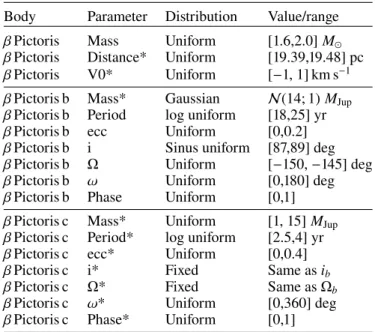
Table 2. Priors used for our MCMC fittings.
Body Parameter Distribution Value/range
β Pictoris Mass Uniform [1.6,2.0] M
β Pictoris Distance* Uniform [19.39,19.48] pc
β Pictoris V0* Uniform [−1, 1] km s−1
β Pictoris b Mass* Gaussian N (14; 1) MJup
β Pictoris b Period log uniform [18,25] yr
β Pictoris b ecc Uniform [0,0.2]
β Pictoris b i Sinus uniform [87,89] deg
β Pictoris b Ω Uniform [−150, −145] deg
β Pictoris b ω Uniform [0,180] deg
β Pictoris b Phase Uniform [0,1]
β Pictoris c Mass* Uniform [1, 15] MJup
β Pictoris c Period* log uniform [2.5,4] yr
β Pictoris c ecc* Uniform [0,0.4]
β Pictoris c i* Fixed Same as ib
β Pictoris c Ω* Fixed Same as Ωb
β Pictoris c ω* Uniform [0,360] deg
β Pictoris c Phase* Uniform [0,1]
Notes. The priors labeled with an * apply only when the RVs are considered (NIRDIFS-GRAV-RV case).
Unless otherwise specified, we adopted a distance to the star of 19.44 pc (HIPPARCOSdistance) when dealing with astromet-ric data only, even though Gaia DR2 provided a more recent estimate. This is to allow for a comparison with other works; this is also because the Gaia DR2 parallax has a larger uncertainty than the HIPPARCOSone due to its saturation, and because the time baseline to model this three-component system is a factor of two lower than the HIPPARCOSone.
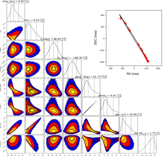
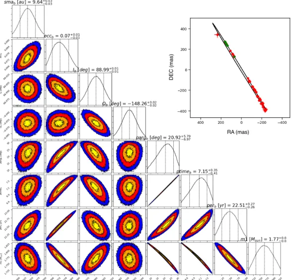
The results are displayed in Fig. 3. The sma, eccentricity, and mass distributions are not symmetrical and cannot be fitted by Gaussian profiles. We note this was also the case in previous studies based on SPHERE or GPI results. The sma distribution peaks at 9 au and has a small wing at larger values. We note that this wing is much shallower than inLagrange et al.(2019a). The eccentricity peaks slightly below 0.01, with a wing toward larger values; this barely rejects a zero eccentricity. The distribution of inclinations can be fitted by a Gaussian profile, with a maximum at 88.94 deg and one sigma of 0.04 deg. The star mass distri-bution peaks at 1.77 M , with a wing toward lower values. The obtained orbital elements compare well with those described in
Lagrange et al.(2019a), as well as with those derived from case 2 using NACO and newly recalibrated GPI data fromNielsen et al.
(2020) (who used the HIPPARCOS distance). The mass of the star derived byNielsen et al.(2020) (case 1) is also comparable. Their eccentricity does not show a peak, but a steady decrease starting from zero.
We now check how these posteriors depend on the various assumptions or inputs by:
– Assuming a Gaia distance, in the range of [19.63,19.88] pc, would lead to an sma distribution peaking at 9.17 au and a star mass peaking at 1.83 M .
– Removing the two data points closest to the star4 obtained in Nov 2016 (proj. sep 130 mas) and Sept 2018 (proj. sep 140 mas), that is, at the last observation before the closest
4 Indeed, being so close to the star, one could expect the planet
astrom-etry to be more impacted by data reduction effects due to, e.g., stronger self subtraction and a higher slope in the stellar halo.
approach and the first observation after the closest approach does not change the results.
– Considering the IRDIS (average of method 1 and method 2 results) and IFS (method 1) data separately gives poste-riors that are compatible within the uncertainties with the NIRDIFS case above; yet, we notice that (1) the median sma and median eccentricity are slightly shifted toward higher values when only using IRDIS data, as opposed to when only using IFS data, and the star mass is slightly lower, and that (2) the posteriors obtained when only using IFS data are closer to those obtained with both IRDIS and IFS (NIRDIFS) than the posteriors obtained using only IRDIS. This is because the IFS measurements are associated with smaller error bars than for the IRDIS measurements. – Finally, using the PACO measurements or the measurements
obtained with method 1 as inputs for the IFS data only leads to compatible results, but with a slightly higher median eccentricity, 0.035.
In conclusion, the data (IFS versus IRDIS) and the methods used to measure the relative astrometry of β Pictoris b slightly impact the posteriors, but the results are still compatible. Due to the smaller error bars, the IFS measurements (method 1) used in the NIRDIFS case dominate the astrometric information over the IRDIS data. The assumption on the distance to the star also impacts the orbital parameters and the star mass.
3.2. Analysis of HCI and GRAVITY data
We ran new MCMCs taking into account the relative astro-metric data provided by GRAVITY on β Pictoris b in addition to the IRDIFS data. This new data set is hereafter referred to as NIRDIFS-GRAV. The obtained sma, eccentricity, and mass distributions are more symmetrical than when only using the NIRDIFS measurements, as seen in Fig. 4. For the sma, we derived a value of 9.64 ± 0.04 au, for the eccentricity, a value of 0.07 ± 0.01, and for the inclination, a value of 88.99 ± 0.01 deg. The star mass is 1.77 ± 0.03 M . Similar values are obtained without taking into account the Nov. 2016 and Sept. 2018 data. When considering the IRDIS and IFS (method 1) measurements separately, or when using the PACO measurements instead of the IFS method 1 ones, we obtain the same tendencies as in the pre-vious section, with even smaller differences. The posteriors are now clearly driven by the GRAVITY data points5
Finally, we then assumed the Gaia distance instead of the
HIPPARCOS one. We got a higher sma (+0.15 au), a similar
eccentricity, and a higher star mass (+0.09 M ).
The posteriors found here with NIRDIFS-GRAV are in qualitative-only agreement with those found by GRAVITY Collaboration (2020) from the relative astrometry: sma = 10.6 ± 0.5 au, e = 0.15 ± 0.4, and M = 1.82 ± 0.3 M . This can be explained by a combination of various differences: (1) dif-ferent HCI data were used (GPI instead of SPHERE), (2) the GPI data suffered from calibration errors (seeNielsen et al. 2020
for the revised values), (3) we use, in the present paper, six
5 As an exercise, we performed the MCMC analysis using GRAVITY
data alone as input and using the same priors as before; it turns out that even though they are much less precise (larger uncertainties), the pos-teriors are compatible with those found in our NIRDIFS-GRAV case, where we used more than 12 yr of HCI data. This illustrates the impact of the GRAVITY data, thanks to their exquisite precision. It has to be noted, though, that GRAVITY needs the HCI data to point and place the fiber at the rough position of the planet before any measurements can be carried out. Both data are then complementary.
D EC (ma s) RA (mas) +
Fig. 3.Results of the MCMC analysis of the NACO + IRDIFS astrometric data. From top to bottom: sma, eccentricity, inclination, longitude of
the ascending node, argument of periastron, periastron time, period of β Pictoris b, and star mass. A distance of 19.44 pc is assumed. The orbital solutions are shown in the upper right. The vertical-dashed lines, from left to right, indicate the 16, 50, and 84% quantiles. The values on top of each histogram are the median+(84%quantile−50%quantile)−(50%quantile−16%quantile).
pieces of GRAVITY data instead of one, and (4) the value of the GRAVITY astrometry used inGRAVITY Collaboration(2020) has been slightly revised for the present paper.
In conclusion, adding the GRAVITY data to the NACO and SPHERE data leads to significantly different orbital parame-ters and, specifically, higher values of sma and eccentricity for β Pictoris b. The star mass is between that proposed by Crifo et al.(1997), based on photometry and the HIPPARCOSdistance and that proposed byZwintz et al.(2019) based on an asteroseis-mology study. Using GRAVITY also significantly decreases the fitting uncertainties associated to the orbital parameters, thanks to small error bars. GRAVITY, therefore, dominates the rela-tive astrometric information. As a consequence, the results are also dominated by any biases in GRAVITY. The posteriors are also biased by the assumption of a single planet, and we see below that GRAVITY astrometry is sensitive to the influence of β Pictoris c on the relative astrometry of β Pictoris b. Finally, we note that the posteriors still depend on the assumption made on the distance of the system.
3.3. Analysis of HCI, GRAVITY, and RV data
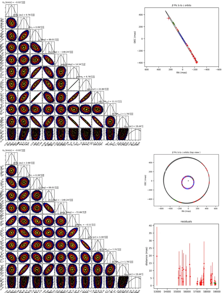
We considered the RV data in addition to the relative astromet-ric data and constrained the properties of β Pictoris b and c. We
used the 32 offsets as input to the MCMC analysis, because using thousands of RV data points in our MCMC analysis would require unrealistically large computing times. In principle, adding the RV data allows one to constrain the masses of both planets in addition to their orbital parameters. We, therefore, added these two additional parameters in our MCMC analysis, and added an RV offset to account for the fact that our RV mea-surements are not absolute velocities, but they are given with respect to a reference spectrum that is built by averaging a large amount of spectra (seeLagrange et al. 2019a).
As we do not have constraints on the inclination of β Pictoris c, we assumed that its orbit is coplanar with that of β Pictoris b. The distance of the system is considered to be uni-form in the [19.39,19.48] pc range, and the mass is uniuni-form within the [1.6,2] M range in the priors. As the GRAVITY precision is typically 0.1 mas, and the total astrometric pertur-bation introduced by β Pictoris c is about 1.5 mas over 3 yr and that introduced by β Pictoris b is about 4 mas over 20 yr, we took these perturbations into account in our MCMC computations, adding up the barycentric corrections due to each planet.
We first ran an MCMC analysis, using a uniform distribu-tion for the masses of β Pictoris b and c in the [1,20] MJuprange, and ended up with a posterior for β Pictoris c’s mass of 7.7 MJup, that is, close to the estimate given in Lagrange et al.(2019a).
D EC (ma s) RA (mas) + +
Fig. 4.Results of the MCMC analysis of the NACO + IRDIFS + GRAVITY astrometric data. From top to bottom: sma, eccentricity, inclination,
longitude of the ascending node, argument of periastron, periastron time, period of β Pictoris b, and star mass. A distance of 19.44 pc is assumed. The orbital solutions are shown in the upper right: NIRIFS data (red) and GRAVITY data (green). The vertical-dashed lines indicate, from left to right, the 16, 50, and 84% quantiles. The values on top of each histogram are the median+(84%quantile−50%quantile)−(50%quantile−16%quantile).
Yet, the posterior on the mass of β Pictoris b is 3.2 MJup, which is not compatible with any luminosity-mass relation or any pre-vious related estimate. Additionally, this is not compatible with the fact that we did not detect β Pictoris c in single direct images when at quadrature, as expected at about 150 mas, while we did, in fact, detect β Pictoris b at smaller projected separations6. With our current knowledge, we attribute this poor constraint on β Pictoris b’s mass to the fact that (1) the RV time series does not fully cover β Pictoris b’s period as seen in the third row of Fig.27) and (2) the data have non-negligible noise.
We used a prior of a Gaussian, centered on 14 MJup, and a one-sigma of 1 MJup(noted hereafter N(14,1)) for β Pictoris b’s mass. This range is representative of the high masses estimated for β Pictoris b in the literature. The results are summarized in TableC.4 and visualized in Figs.5 and6. For β Pictoris b, we
6 We note that for this last argument, we assume that both planets
formed in the same way.
7 In this figure, the RV induced by the planets correspond to the
solu-tions obtained in the case where the mass of β Pictoris b is constrained in a Gaussian range (14,1), as described below. In the present case, the mass found for β Pictoris b is 3 MJup, and its impact on the RV would be
even smaller.
find an sma of 9.76 ± 0.04 au, an eccentricity of 0.086 ± 0.006, and an inclination of 89.01 ± 0.01 deg. For β Pictoris c, we find an sma of 2.69 ± 0.02 au, and an eccentricity of 0.27 ± 0.07. The star mass is 1.78 ± 0.03 M and the distance is 19.44 ± 0.02 pc. The orbital parameters of β Pictoris c are in good agreement with those found inLagrange et al.(2019a), where we analyzed only the RV data and made some assumptions about β Pictoris b to correct the RV data from this planet contribution. The masses found for planets b and c are 11.1 ± 0.8 and 7.8 ± 0.4 MJup, respectively. We see, in Fig.2(bottom) that the time baseline is now long enough to possibly see the impact of β Pictoris b on the RV through a modulation of the β Pictoris c induced RV curve.
To investigate the impact of the prior on β Pictoris b’s mass, we performed a similar MCMC analysis with a Gaussian N(12,1) MJupprior. We ended up with a mass of 9.7 ± 0.7 MJupfor β Pictoris b, which is significantly lower than when using the (14,1) MJupprior and an unchanged mass for β Pictoris c. This confirms that β Pictoris b’s mass is not fully constrained yet, while the mass of β Pictoris c is.
To investigate the impact of the RV precision on the results, we set a threshold of 15 m s−1 to the RV uncertainties, that is, all uncertainties lower than 15 m s−1 were set at 15 m s−1. The
Fig. 5.Results of the MCMC analysis of the NIRDIFS + GRAVITY + RV data. Top: β Pictoris b. Bottom: β Pictoris c. For each planet and from top to bottom: sma, eccentricity, inclination, longitude of the ascending node, argument of periastron, periastron time, period and mass of the planet, star mass, and distance. The vertical-dashed lines indicate, from left to right, the 16, 50, and 84% quantiles. The values on top of each histogram are the median+(84%quantile−50%quantile)−(50%quantile−16%quantile). The orbital solutions are encapsulated in the top and bottom figures. The average of the residuals of the astrometric fits (distances) are provided as well.
Fig. 6.Results of the MCMC analysis of the NIRDIFS+GRAVITY + RV data. Top: fit of the RV offsets (left). For comparison purposes, the fit of the RV offsets in an MCMC run without priors on β Pictoris b’s mass is provided (right). Bottom: residuals of the corresponding RV fits.
only noticeable impact was an increase in β Pictoris b’s mass of 0.5 MJupand a decrease in β Pictoris c’s mass of 0.5 MJup. Run-ning a test adding 15 m s−1 to all initial uncertainties increases the mass of β Pictoris b by 1.5 MJupand the mass of β Pictoris c by only 0.2 MJup(i.e., barely outside the 1-sigma uncertainties), and it increases the eccentricity of β Pictoris c from 0.28 to 0.34. These last tests illustrate how critically the RVs constrain the mass of the planets. Another illustration is provided in Fig. 6
where we show both the RV curves corresponding to our fits of the NIRDIFS-GRAV-RV data, when using a N(14,1) prior (left) and when using a flat prior (right) on β Pictoris b’s mass. They give posteriors of 11 and 3.2 MJup, respectively, for β Pictoris b mass. We see that the RV curve corresponding to the lower mass for β Pictoris b fits the offsets in a slightly better way than the other one, but the difference is small. Longer time base-lines for the RV, a better coverage of the RV at both β Pictoris c quadratures, and/or a better precision on the offsets (through a better removal of the stellar pulsations) will help further con-strain the mass of β Pictoris b. Gaia full data (IADs) will also help constrain the planet masses.
To investigate the impact of the star distance, we ran an MCMC analysis, assuming the Gaia distance range of [19.63,19.88] pc. Compared to the posteriors obtained using the
HIPPARCOSdistance, the sma of β Pictoris b and c are slightly
increased by, respectively, +0.16 au, which has yet to be com-pared to the uncertainties of 0.04 au, and +0,04 au, which has yet to be compared to the uncertainties of 0,02 au. The stellar
mass is now 1.87 ± 0.04 M , compared to 1.77 ± 0.03 M . The masses of β Pictoris b and c are only marginally increased, and they remain consistent given the uncertainties.
4. Discussion
The present analysis provides significantly improved orbital parameters for β Pictoris b, compared to previous studies, as well as a good estimate of the orbital properties of β Pictoris c. We note that (1) the eccentricity obtained for β Pictoris c (0.27) might be overestimated due to the limited signal-to-noise of the RV data and their temporal sampling (see Shen & Turner 2008), and (2) even with this eccentricity, its orbit would be dynamically stable.
As seen before, the mass of β Pictoris b is poorly constrained and additional long observing RV sequences (typically 3-6 h long each night on three continuous nights) over a few more years are needed to measure this dynamical mass. An improved correction of the pulsations would also allow for a better mass estimate. Previous studies have used HIPPARCOS-Gaia data to constrain the mass of β Pictoris b, but only using one planet in their fit, which is not adapted. We, therefore, attempted to use
HIPPARCOS-Gaia to further constrain the mass of this planet.
We conclude that the RV data fully drives the solution on the planet masses, as detailed in AppendixB.
On the contrary, β Pictoris c M · sin i is much better con-strained. This is because the period of planet c is much smaller
101 100 101 102 sma (au) 2.5 5.0 7.5 Ma ss 0.1 0.5 0.68 0.9 101 100 101 102 sma (au) 2.5 5.0 7.5 Ma ss 0.1 0.5 0.68 0.9
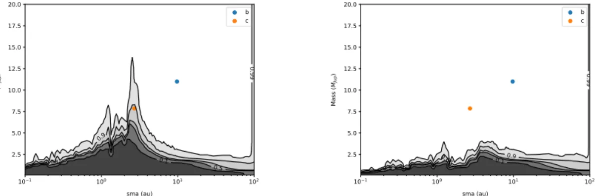
Fig. 7. Left: detection probabilities of planets around β Pictoris using all available HCI data and RV pulsation-subtracted data. Right: detection
probabilities of planets around β Pictoris using all available HCI data and RV data which were pulsation-subtracted and corrected from β Pictoris b and c. Various levels of probabilities are considered. The two known planets are indicated.
than that of planet b, and it has a much better temporal coverage over its period. The present data do not allow for one to constrain the inclination of the planet orbit, but a significant inclination would be very surprising.
This work allowed us to estimate the previous and next tran-sit times for both planets. Using the fit of NIRDIFS-GRAV-RV, and assuming a Gaussian distribution N(14,1) for β Pictoris b, we find that the last transit of β Pictoris b occurred on Sept 2017, and that of β Pictoris c occurred on Nov 2017. The next transit of β Pictoris b will occur in July-August 2040 and that of β Pictoris c in March 2021. The dates vary within a few days for the next transit of β Pictoris c and months for β Pictoris b if we change the hypothesis on β Pictoris b’s mass, on the star distance, and even more if we change the “thresholded” RV (see above).
Given the mass of β Pictoris c and using COND03 models, we find an absolute magnitude of 12.7 at H band and, hence, we expect a 10.7 mag contrast with the star. Given the mea-sured magnitude of β Pictoris b at H band, we expect a contrast of 0.8–0.9 mag between both planets (hence a flux ratio of 6–8). We examined the possibility of direct detection of β Pictoris c in our SPHERE data, using the positions computed with the orbital parameters found in the previous section. Even if this is not an independent confirmation of its presence, detecting a signal at the planet position would be useful because it would set the rel-ative inclination of the two orbits and provide an estimate of the relative contrast.
It appears that at most epochs, the projected position of β Pictoris c is behind the coronagraphic mask. The projected separation is greater than 100 mas in the following months: Dec. 2014; Feb. 2015; Sept. Oct, and Nov. 2016; Sept., Oct., and Dec. 2018; Dec. 2019; and Jan. 2020. Yet, in Sept., Oct., and Nov. 2016 and Sept., Oct., and Dec. 2018, the two planets are within 3 pixels (with a separation down to 9 mas in Nov. 2016) in the plane of the sky. We are then left with four epochs in which the planet is expected to be out of the coronagraph and sufficiently far from b: Feb. 2015 and Dec. 2018, when it should be NE of the star, as well as Dec. 2019 and Feb. 2020, when it is expected to be SW of the star. An examination of the corresponding images does not clearly reveal β Pictoris c. Further work will include the combination of all data set, for example, as done inLe Coroller et al.(2020) to try and directly detect β Pictoris c in the SPHERE data.
5. Additional planets in the β Pictoris system
Here, we used all available (25) high contrast IRDIS images obtained with NACO and SPHERE and combined them with our
7000+ pulsation-corrected RVs to estimate the probability of the presence of other planets in the system. The approach is the same as the one described inLagrange et al.(2018) where we used 7 NACO and 2100 pieces of RV data available up to 2016. In a nut-shell, we generated (Monte Carlo) planets with various orbital properties and masses and tested whether these simulated plan-ets are detected at least for one epoch in direct imaging or if they are detected in RV data. In direct imaging, the planet is detected if its flux (derived from COND03 brightness-mass relationships,
Baraffe et al. 2003) is higher than the three-sigma above noise in a given image. For the RV, we computed the RV series associ-ated to each simulassoci-ated planet at the time of observations and we tested whether the planet is or is not detectable by comparison with the observed RV time-series (see details in Lannier et al. 2017). InLagrange et al.(2018), we used NACO L’ data only. We upgraded the code to be able to combine images obtained with different instrumental set-ups. The results are given in Fig.7. The comparison with Fig. 5 ofLagrange et al.(2018) shows the tremendous improvement in detection limits, with detection lim-its reduced by a factor of 2–4 at almost all separations. To obtain tighter limits, we subtracted the β Pictoris b and c RV signals from the pulsation-corrected data, using the parameters found in the previous section. The result is shown in Fig.7. From this fig-ure, we can exclude, with a probability greater than 90%, planets that are more massive than about 2.5 MJupcloser than 3 au, and those that are more massive than 3.5 MJupbetween 3 and 7.5 au. The intermediate region will be further constrained by the Gaia final release.
The present study shows that there are no massive planets in the system, other than β Pictoris b and c, and that the overall dynamics of the β Pictoris system is controlled by β Pictoris b and c. This property could help us to achieve a better con-straint on their orbits. The β Pictoris b and c system can indeed be considered as dynamically isolated from the rest of the disk. A stability analysis that eliminates the unstable configurations could help us refine our knowledge of the orbits.
Using the estimates ofLazzoni et al.(2018) of chaotic zones of planets (Mustill & Wyatt 2012), we find that the presence of β Pic b and c with masses of 11 and 7.8 MJup, sma of 9.8 and 2.7 au, and eccentricities of 0.08 and 0.28, respectively, is enough to clear out the material in the inner 10 au region. We now focus on the region beyond 10 au.
The planetesimal belt in the β Pic disk is located between 50– 130 au (Augereau et al. 2001;Dent et al. 2014). Assuming that the belt initially extended down to the inner region, we could set a lower limit to the masses of planets that could be hidden in the inner region and that could have cleared a gap in about
20 Myr. We based our calculations on the numerical simulations byShannon et al.(2016), which show that two planets of a min-imum of 0.3 MJup would be needed between β Pic b and the inner location of the outer planetesimal belt to explain the cav-ity. There can, therefore, be two additional planets with masses between 0.3 and 2.5 MJup between 10 and 50 au that could be explored further observationally using more SPHERE data and combining them as in this present work, or more sensitive instru-ments on the JWST or on the ELT. We note that gas observations in β Pic (Matrà et al. 2017; Cataldi et al. 2018) show that the atomic gas does not extend in the inner regions, as expected from previous models (Kral et al. 2016,2017), and it is mainly colocated with the outer planetesimal belt, which may be a sign that viscous spreading is halted by a planet inward of 50 au, as demonstrated inKral et al.(2020).
6. Concluding remarks and perspectives
We obtained new astrometric data on β Pictoris b with SPHERE in high contrast direct imaging and with GRAVITY in long base interferometry, as well as new RV data. The new RV data confirm the detection of β Pictoris c, and the modulation of the RV data by β Pictoris b is becoming visible.
We combined these HCI, GRAVITY, and RV data, as well as previously published data, in a single MCMC analysis to constrain the orbital properties of both planets. The orbital prop-erties of β Pictoris b are driven by the GRAVITY measurements, which have much smaller uncertainties than the HCI ones. This illustrates the exquisite complementarity between both tech-niques. We confirm that β Pictoris b has a small but nonzero eccentricity (0.09 ± 0.01) and it does not transit the star. The orbital properties of β Pictoris c are well constrained, provided its orbital plane indeed coincides with that of β Pictoris b. The mass of β Pictoris c is well constrained at 7.8 ± 0.4 MJup, assuming both orbits of the planets are coplanar.
While the orbital properties of β Pictoris b are now well con-strained, its mass is not. This is because the baseline of the RV data is still shorter than the planet period, and the data are noisy. Additional data recorded with our updated observing strategy will allow constraining β Pictoris b’s mass.
The absolute astrometry HIPPARCOS-Gaia data are con-sistent with the solutions presented here at the 2σ level, but these solutions are fully driven by the relative astrometry plus RV data. HIPPARCOS-Gaia data should help to further con-strain β Pictoris b’s mass once more detailed Gaia data are available.
Using the NACO and IRDIS HCI images as well as the RV data, once the pulsations and the signals of β Pictoris b and c were corrected for, we computed the detection limits of addi-tional planets in the system. We can now exclude the presence of planets that are more massive than about 2.5 MJupcloser than 3 au, and more massive than 3.5 MJupbetween 3 and 7.5 au. This represents an improvement of more than 5–10 in detection limits compared to our previous study in the 1–10 au region. Between 10 and 100 au, we exclude planets with masses of 1–2 MJup. We conclude that the dynamics of the system as a whole is con-trolled by β Pictoris b and c, and that additional planets with masses equal to or less than Jupiter mass have to be present to explain the inner void of material in the 10–70 au region. They certainly represent interesting targets for forthcoming JWST and ELT observations. Finally, given the properties found in this paper, β Pictoris b and c can explain the relative void of material in the inner 10 au disk.
Acknowledgements. We acknowledge support from the French CNRS, from the Agence Nationale de la Recherche (ANR-14-CE33-0018), and the OSUG LABEX. A.V. and G.O. acknowledge funding from the European Research Council (ERC) under the European Union’s Horizon 2020 research and inno-vation programme (grant agreement No. 757561). A.A. and P.G. were sup-ported by Fundação para a Ciência e a Tecnologia, with grants reference UIDB/00099/2020 and SFRH/BSAB/142940/2018. R.G.L. acknowledges sup-port by Science Foundation Ireland under Gant. No. 18/SIRG/5597. Based on observations collected at the European Southern Observatory under ESO programmes 0104.C-0418(D), 0104.C-0418(E), 0104.C-0418(F), 1104.C-0651, 098.C-0739(A), 0104.C-0418(A), 0104.C-0418(C).
References
Arenou, F., Luri, X., Babusiaux, C., et al. 2018,A&A, 616, A17
Augereau, J. C., Nelson, R. P., Lagrange, A. M., Papaloizou, J. C. B., & Mouillet, D. 2001,A&A, 370, 447
Baraffe, I., Chabrier, G., Barman, T. S., Allard, F., & Hauschildt, P. H. 2003,
A&A, 402, 701
Beust, H., & Morbidelli, A. 1996,Icarus, 120, 358
Beust, H., & Morbidelli, A. 2000,Icarus, 143, 170
Beuzit, J. L., Vigan, A., Mouillet, D., et al. 2019,A&A, 631, A155
Bonnefoy, M., Marleau, G.-D., Galicher, R., et al. 2014,A&A, 567, L9
Brandt, T. D. 2018,ApJS, 239, 31
Cataldi, G., Brandeker, A., Wu, Y., et al. 2018,ApJ, 861, 72
Chauvin, G., Desidera, S., Lagrange, A.-M., et al. 2017,A&A, 605, L9
Claudi, R. U., Turatto, M., Gratton, R. G., et al. 2008,SPIE Conf. Ser., 7014, 3
Crifo, F., Vidal-Madjar, A., Lallement, R., Ferlet, R., & Gerbaldi, M. 1997,A&A, 320, L29
Delorme, P., Schmidt, T., Bonnefoy, M., et al. 2017,A&A, 608, A79
Dent, W. R. F., Wyatt, M. C., Roberge, A., et al. 2014, Science, 343, 1490
Dohlen, K., Langlois, M., Saisse, M., et al. 2008,SPIE Conf. Ser., 7014, 3
Dupuy, T. J., Brandt, T. D., Kratter, K. M., & Bowler, B. P. 2019,ApJ, 871, L4
Flasseur, O., Denis, L., Thiébaut, É., & Langlois, M. 2020,A&A, 637, A9
Foreman-Mackey, D., Hogg, D. W., Lang, D., & Goodman, J. 2013,PASP, 125, 306
Gaia Collaboration (Brown, A. G. A., et al.) 2018,A&A, 616, A1
Galicher, R., Boccaletti, A., Mesa, D., et al. 2018,A&A, 615, A92
Galland, F., Lagrange, A.-M., Udry, S., et al. 2005,A&A, 443, 337
Grandjean, A., Lagrange, A. M., Beust, H., et al. 2019,A&A, 627, L9
GRAVITY Collaboration (Abuter, R., et al.) 2017,A&A, 602, A94
GRAVITY Collaboration (Lacour, S., et al.) 2019,A&A, 623, L11
GRAVITY Collaboration (Nowak, M., et al.) 2020,A&A, 633, A110
Kervella, P., Arenou, F., Mignard, F., & Thévenin, F. 2019, A&A, 623, A72
Kiefer, F., Lecavelier des Etangs, A., Boissier, J., et al. 2014, Nature, 514, 462
Kral, Q., Wyatt, M., Carswell, R. F., et al. 2016,MNRAS, 461, 845
Kral, Q., Matrà, L., Wyatt, M. C., & Kennedy, G. M. 2017,MNRAS, 469, 521
Kral, Q., Davoult, J., & Charnay, B. 2020,Nat. Astron., 4, 769
Kristensen, K., Nielsen, A., Berg, C., Skaug, H., & Bell, B. 2016,J. Stat. Soft. Art., 70, 1
Lacour, S., Dembet, R., Abuter, R., et al. 2019,A&A, 624, A99
Lagage, P. O., & Pantin, E. 1994,Nature, 369, 628
Lagrange, A.-M., Bonnefoy, M., Chauvin, G., et al. 2010,Science, 329, 57
Lagrange, A.-M., De Bondt, K., Meunier, N., et al. 2012,A&A, 542, A18
Lagrange, A. M., Keppler, M., Meunier, N., et al. 2018,A&A, 612, A108
Lagrange, A. M., Boccaletti, A., Langlois, M., et al. 2019a,A&A, 621, L8
Lagrange, A. M., Meunier, N., Rubini, P., et al. 2019b, Nat. Astron., 3, 1135
Lannier, J., Lagrange, A. M., Bonavita, M., et al. 2017,A&A, 603, A54
Lapeyrere, V., Kervella, P., Lacour, S., et al. 2014,Proc. SPIE, 9146 , 91462D
Lazzoni, C., Desidera, S., Marzari, F., et al. 2018,A&A, 611, A43
Le Coroller, H., Nowak, M., Delorme, P., et al. 2020,A&A 639, A113
Lindegren, L., Hernández, J., Bombrun, A., et al. 2018,A&A, 616, A2
Macintosh, B. A., Graham, J. R., Palmer, D. W., et al. 2008,SPIE Conf. Ser., 7015, 701518
Marois, C., Lafrenière, D., Doyon, R., Macintosh, B., & Nadeau, D. 2006,ApJ, 641, 556
Marrese, P. M., Marinoni, S., Fabrizio, M., & Altavilla, G. 2019,A&A, 621, A144
Matrà, L., Dent, W. R. F., Wyatt, M. C., et al. 2017,MNRAS, 464, 1415
Mustill, A. J., & Wyatt, M. C. 2012,MNRAS, 419, 3074
Nielsen, E. L., De Rosa, R. J., Wang, J. J., et al. 2020,AJ, 159, 71
van Leeuwen, F. 2007,A&A, 474, 653
van Leeuwen, F., & Evans, D. W. 1998,A&AS, 130, 157
Vigan, A., Moutou, C., Langlois, M., et al. 2010,MNRAS, 407, 71
Wahhaj, Z., Koerner, D. W., Ressler, M. E., et al. 2003,ApJ, 584, L27
Woillez, J., & Lacour, S. 2013,ApJ, 764, 109
Zurlo, A., Vigan, A., Mesa, D., et al. 2014,A&A, 572, A85
Zurlo, A., Vigan, A., Galicher, R., et al. 2016,A&A, 587, A57
Zwintz, K., Reese, D. R., Neiner, C., et al. 2019,A&A, 627, A28
1 IPAG, Univ. Grenoble Alpes, CNRS, IPAG, 38000 Grenoble, France
e-mail: [email protected]
2 LESIA, Observatoire de Paris, Université PSL, CNRS, Sorbonne
Université, Université de Paris, 5 place Jules Janssen, 92195 Meudon, France
3 IMCCE – Observatoire de Paris, 77 Avenue Denfert-Rochereau,
75014 Paris, France
4 Pixyl, 5 Avenue du Grand Sablon, 38700 La Tronche, France 5 Institute of Astronomy, University of Cambridge, Madingley Road,
Cambridge CB3 0HA, UK
6 CRAL, UMR 5574, CNRS, Université de Lyon, Ecole Normale
Supérieure de Lyon, 46 Allée d’Italie, 69364 Lyon Cedex 07, France
7 INAF – Osservatorio Astronomico di Padova, Vicolo dellâ
Osserva-torio 5, 35122, Padova, Italy
8 Department of Astronomy, California Institute of Technology,
Pasadena, CA 91125, USA
9 GEPI, Observatoire de Paris, PSL University, CNRS; 5 Place Jules
Janssen 92190 Meudon, France
10 Aix-Marseille Univ, CNRS, CNES, LAM, Marseille, France 11 Núcleo de Astronomía, Facultad de Ingeniería, Universidad Diego
Portales, Av. Ejercito 441, Santiago, Chile
12 STAR Institute/Université de Liège, Liège, Belgium
13 Max Planck Institute for Astronomy, Königstuhl 17, 69117
Heidelberg, Germany
14 European Southern Observatory, Casilla 19001, Santiago 19, Chile
Universidad de Chile, Casilla 36-D, Santiago, Chile
18 School of Physics and Astronomy, Monash University, Clayton, VIC
3800, Melbourne, Australia
19 Leiden Observatory, Leiden University, PO Box 9513, 2300 RA
Leiden, The Netherlands
20 Max Planck Institute for extraterrestrial Physics, Gießenbachstraße
1, 85748 Garching, Germany
21 Institute of Physics, University of Cologne, Zülpicher Straße 77,
50937 Cologne, Germany
22 Max Planck Institute for Radio Astronomy, Auf dem Hügel 69,
53121 Bonn, Germany
23 Universidade do Porto, Faculdade de Engenharia, Rua Dr. Roberto
Frias, 4200-465 Porto, Portugal
24 School of Physics, University College Dublin, Belfield, Dublin 4,
Ireland
25 Space Telescope Science Institute, Baltimore, MD 21218, USA 26 Geneva Observatory, University of Geneva, Chemin des Mailettes
51, 1290 Versoix, Switzerland
27 Department of Astronomy, Stockholm University, AlbaNova
University Center, 10691 Stockholm, Sweden
28 European Southern Observatory, Karl-Schwarzschild-StraßBe 2,
85748 Garching, Germany
29 Research School of Astronomy & Astrophysics, Australian National
University, ACT 2611, Australia
30 Center for Astrophysics | Harvard & Smithsonian, Cambridge, MA
02138, USA
31 INAF – Osservatorio Astrofisico di Catania, Via S. Sofia 78, 95123
Catania, Italy
32 Astronomy Department, University of Michigan, Ann Arbor, MI
48109, USA
33 Cornell Center for Astrophysics and Planetary Science, Department
of Astronomy, Cornell University, Ithaca, NY 14853, USA
34 Hamburger Sternwarte, Gojenbergsweg 112 21029 Hamburg,
Germany
35 Institute for Particle Physics and Astrophysics, ETH Zurich,
Appendix A: Fits of the RV data #14 <Time>=4525.524 0.50 0.55 0.60 0.65 0.70 Time (days) -1000 -500 0 500 1000 RV (m/s) #15 <Time>=4786.621 0.60 0.65 0.70 0.75 0.80 0.85 0.90 Time (days) -1000 -500 0 500 1000 RV (m/s) #15 <Time>=4787.628 0.60 0.65 0.70 0.75 0.80 Time (days) -1000 -500 0 500 1000 RV (m/s) #15 <Time>=4789.612 0.610 0.615 0.620 0.625 0.630 0.635 Time (days) -1000 -500 0 500 1000 RV (m/s) #16 <Time>=4827.609 0.60 0.65 0.70 0.75 0.80 0.85 0.90 Time (days) -1000 -500 0 500 1000 RV (m/s) #16 <Time>=4828.587 0.55 0.60 0.65 0.70 0.75 0.80 0.85 Time (days) -1000 -500 0 500 1000 RV (m/s) #16 <Time>=4829.606 0.60 0.65 0.70 0.75 0.80 0.85 Time (days) -1000 -500 0 500 1000 RV (m/s) #17 <Time>=4905.507 0.50 0.52 0.54 0.56 0.58 0.60 Time (days) -1000 -500 0 500 1000 RV (m/s) #17 <Time>=4906.502 0.50 0.52 0.54 0.56 0.58 Time (days) -1000 -500 0 500 1000 RV (m/s) #17 <Time>=4908.517 0.50 0.52 0.54 0.56 0.58 Time (days) -1000 -500 0 500 1000 RV (m/s) #17 <Time>=4909.530 0.53 0.54 0.55 0.56 0.57 Time (days) -1000 -500 0 500 1000 RV (m/s) #18 <Time>=4921.501 0.50 0.55 0.60 0.65 0.70 Time (days) -1000 -500 0 500 1000 RV (m/s) #18 <Time>=4922.492 0.48 0.50 0.52 0.54 0.56 0.58 0.60 0.62 Time (days) -1000 -500 0 500 1000 RV (m/s) #18 <Time>=4923.491 0.45 0.50 0.55 0.60 0.65 0.70 Time (days) -1000 -500 0 500 1000 RV (m/s)
Fig. A.1.Fits of the RV data for each observing epoch. The various epochs of observations are indicated on the top of each figure, with numbers
from 14 to 18, as well as the average time over this epoch. We note that sequences with the same number belong to the same epoch and were fitted together.
Appendix B: On the use of HIPPARCOS-Gaia data
We used the Template Model Builder (TMB8,Kristensen et al. 2016), which implements automatic differentiation (AD), to robustly and quickly solve nonlinear models. This fast method
8 http://www.admb-project.org/
allowed us to use all the 7000 RV points and to implement an accurate handling of the Gaia data. Indeed the Gaia DR2 data (Gaia Collaboration 2018) only provides the five astrometric parameters solution obtained assuming a single star model. To simulate how these five parameters are influenced by the configu-ration of the system, we simulated the Gaia observations and it’s five parameter solution. For each epoch of observation of Gaia
tion was simply derived through a linear least squares solution (e.g.,van Leeuwen & Evans 1998). Generating such a solution for each MCMC trial can be cumbersome, but it is quick for the AD method.
To be able to combine the HIPPARCOSIAD ofvan Leeuwen
(2007) with Gaia DR2 data, we needed to first put both sys-tems in the same reference frame, in terms of proper motions (Lindegren et al. 2018; Brandt 2018; Kervella et al. 2019) and of the parallax zero point (Arenou et al. 2018). For simplicity in the handling of the HIPPARCOSIAD, we converted the Gaia DR2 data to the HIPPARCOS reference system. To derive the rotations, we used the 1 arcsec cone search HIPPARCOS-Gaia cross-match described inMarrese et al.(2019) and selected only the HIPPARCOSstars not already known to be binaries (same sample as used inArenou et al. 2018). We tested that using this full sample and we obtain rotations consistent withBrandt(2018) andKervella et al.(2019). We found a significant variation of the rotation with magnitude and a smaller one with color. As we do not have enough bright stars in common to select on both mag-nitude and color, we concentrated only on the main magmag-nitude effect and selected all stars with G < 5. We derived the follow-ing rotations: the first one is from the proper motion derived from the Gaia-HIPPARCOS position difference divided by the ∼24-yr baseline (HG) to the HIPPARCOSproper motion system:
ωHG2Hip = (0.071, −0.142, −0.057) with an uncertainty on each
of those coefficients of around 0.02; the second one is from the
9 https://www.cosmos.esa.int/web/Gaia/
scanning-law-pointings
G H
estimated in a magnitude-dependant way (Lindegren et al. 2018;
Arenou et al. 2018) with an additive term for HIPPARCOSand an inflation factor for Gaia (Brandt 2018). Using our bright sam-ple, we derived an additive term of σ = 0.36 mas and an inflation factor of the Gaia errors of 2.1. Those were applied to the covari-ance matrix of the Gaia DR2 to derive the log likelihood of the tested parameters. For TMB code simplicity, we neglected the impact of the Rv of Beta Pic on the position propagation from
HIPPARCOSto the Gaia epoch (which is of 0.05 mas).
All the parameters were let free without priors. When we did not fit the HIPPARCOS IADs, we fixed the parallax to the
HIPPARCOSvalue. Else the five astrometric parameters derived
from our code correspond to the system barycenter at J1991.25. As a default starting point for system parameters, we used those of Table C.3, which are unconstrained and a mutual inclina-tion ofNielsen et al.(2020), the HIPPARCOSvalues for the five astrometric parameters, and zero for the RV offset V010. We obtained the same results as with the MCMC method within the quoted uncertainties. We also successfully tested the con-vergence robustness of the TMB method by using the results of the MCMC chains as starting points. From those tests, we con-clude that the RVs are fully driving the solution concerning the mass of the components. Adding the HIPPARCOS-Gaia constrain does not change the results significantly. The HIPPARCOS-Gaia data are consistent with the solutions presented here at the 2σ level.
10 We also implemented the possibility to add an additional offset after
Appendix C: Additional tables
Table C.1. β Pictoris b HCI relative astrometry.
MJD Dec RA Error Dec Error RA Instrument
(mas) (mas) (mas) (mas)
52 953.2 340.18 234.19 31.11 31.11 NACO 55 129.2 −256.46 −153.9 19.79 5.66 NACO 55 194.2 −259.43 −163.91 11.31 12.72 NACO 55 296.2 −299.39 −174.05 9.89 9.90 NACO 55 467.2 −330.32 −194.15 15.55 15.55 NACO 55 516.2 −325.27 −208.14 14.14 11.31 NACO 55 517.2 −329.27 −210.15 19.79 18.38 NACO 55 593.2 −349.26 −212.22 14.14 12.72 NACO 55 646.2 −366.25 −215.28 19.79 16.97 NACO 55 872.2 −390.2 −230.36 18.38 19.79 NACO 55 937.2 −386.16 −242.35 19.79 18.38 NACO 56 257.2 −401.19 −233.4 19.79 19.79 NACO 56 324.14 −386.18 −235.35 14.14 14.14 NACO/AGPM 56 999.23 −294.74 −188.44 3.99 4.40 SPHERE IRDIS 57 058.09 −279.85 −178.94 2.81 2.85 SPHERE IRDIS 57 296.34 −219.89 −143.09 2.98 3.14 SPHERE IRDIS 57 356.25 −202.45 −132.93 3.98 4.23 SPHERE IRDIS 57 382.18 −195.71 −130.96 3.31 3.35 SPHERE IRDIS 57 407.12 −190.28 −124.33 2.56 2.66 SPHERE IRDIS 57 474.02 −168.90 −113.69 2.55 2.62 SPHERE IRDIS 57 494.00 −164.80 −110.39 3.57 3.79 SPHERE IRDIS 57 647.38 −116.28 −79.507 3.76 3.81 SPHERE IRDIS 57 675.35 −108.20 −77.605 3.51 3.56 SPHERE IRDIS 57 710.27 −105.18 −77.255 10.29 10.7 SPHERE IRDIS 58 378.20 123.143 69.87 5.00 5.08 SPHERE IRDIS 58 409.38 138.44 77.0 4.04 3.57 SPHERE IRDIS* 58 467.2 154.926 85.93 3.75 4.12 SPHERE IRDIS* 58 790.30 248.71 142.55 2.27 2.16 SPHERE IRDIS* 58 839.19 258.71 153.56 2.57 2.42 SPHERE IRDIS* 58 887.07 272.59 161.00 1.92 1.83 SPHERE IRDIS* 57 058.09 −282.71 −180.52 1.17 1.17 SPHERE IFS 57 296.34 −217.92 −144.90 1.00 1.00 SPHERE IFS 57 356.25 −202.08 −134.32 1.52 1.52 SPHERE IFS 57 382.18 −196.38 −128.07 1.75 1.75 SPHERE IFS 57 407.12 −187.57 −125.10 1.73 1.73 SPHERE IFS 57 474.02 −168.41 −112.57 1.48 1.48 SPHERE IFS 57 494.00 −161.71 −106.79 1.70 1.70 SPHERE IFS 57 647.38 −116.30 −83.45 2.11 2.11 SPHERE IFS 57 675.36 −111.22 −76.58 2.54 2.54 SPHERE IFS 57 710.25 −83.45 −63.92 4.73 4.73 SPHERE IFS 58 378.35 127.13 68.54 2.92 2.92 SPHERE IFS 58 409.31 135.05 74.61 1.64 1.64 SPHERE IFS* 58 467.19 152.36 85.57 1.22 1.22 SPHERE IFS* 58 552.99 183.03 105.93 1.59 1.59 SPHERE IFS* 58 790.30 246.24 143.83 1.07 1.07 SPHERE IFS* 58 839.20 259.87 151.25 1.17 1.17 SPHERE IFS* 58 887.07 270.94 159.91 0.94 0.94 SPHERE IFS*
58 738.267* 135.403 232.840 0.854 0.094 −0.786 58 796.170* 145.514 248.589 0.108 0.045 −0.823 58 798.356* 145.649 249.210 0.030 0.099 −0.352 58 855.053* 155.476 264.292 0.128 0.292 −0.447 58 855.198* 155.276 264.505 0.053 0.132 −0.278 58 889.139* 160.954 273.418 0.055 0.146 −0.549
Notes. The coefficient ρ is the correlation between the error in RA and in Dec. The covariance matrix can be reconstructed using σ∆RA2 and
σ∆Dec2 on the diagonal, and ρσ∆RAσ∆Decoff-diagonal. The * indicates
new, unpublished data thus far.
780.71 −57 56 799.71 −68 41 829.66 −201 40 851.32 −148 44 913.54 −91 48 1131.79 6 40 1170.70 4 57 1519.79 31 47 1566.70 145 33 1597.62 76 38 2569.81 126 45 2583.38 115 38 2685.70 30 56 2694.56 102 43 2707.08 189 44 2985.24 −6 36 3344.74 −154 59 3668.00 111 40 3712.63 127 27 3770.45 78 16 3849.51 151 40 4007.84 3 35 4037.19 38 7 4064.77 −65 33 4094.64 −32 7 4207.68 −34 10 4233.60 −72 12 4525.58 −87 18 4787.42 −2 9 4828.73 32 5 4907.33 56 15 4922.58 69 8
Table C.4. Posteriors of MCMC fittings (see text).
ab(au) Pb(yr) eb ib(deg) Ωb(deg) ωb(deg) Tpb(yr) Mb(MJup)
ac(au) Pc(yr) ec ic(deg) Ωc(deg) ωc(deg) Tpc(yr) Mc(MJup)
(M∗) (d) V0 (km s−1) NIRDIFS '9.0 (p) '20.3 (p) '0.01(p) 88.94 ± 0.04 −148.31 ± 0.06 '47 (p) '8.7(p) '1.77(p) NIRDIFS-GRAV 9.80 ± 0.04 22.6 ± 0.35 0.08 ± 0.01 88.99 ± 0.01 −148.26 ± 0.02 20.4 ± 6 7.2 ± 0.4 1.835 ± 0.04 NIRDIFS-GRAV-RV 9.76 ± 0.04 22.9 ± 0.25 0.09 ± 0.01 89.01 ± 0.01 −148.24 ± 0.02 14.3 ± 5 6.77 ± 0.3 11.1 ± 0.8 bc-corr, MG14 2.68 ± 0.02 3.0 ± 0.02 0.27 ± 0.06 89.01 ± 0.01 −148.24 ± 0.02 −71.9 ± 13.8 3.01 ± 0.6 7.8 ± 0.4 1.78 ± 0.03 19.4 ± 0.02 −0.016 ± 0.004
Notes. Here, we indicate the mean ± stdev when the distribution is Gaussian, or, otherwise, the position of the peak (noted “(p)”). Tp, expressed in yr, corresponds to the time of periastron passage since JDB = 2 454 000.