Analyzing transient instability phenomena beyond
the classical stability boundary
Mahmoud Ali, Mevludin Glavic, Senior Member, IEEE, Jean Buisson, Member, IEEE,
Louis Wehenkel, Member, IEEE, and Damien Ernst, Member, IEEE
Abstract— We consider power systems for which the amount
of power produced by their individual power plants is small with respect to the total generation of the system, and analyze how the transient instability mechanisms of these systems change qualitatively when their size or the dispersion of their generators increases. Simulation results show that loss of synchronism will propagate more slowly and even stop propagating. Given the evolution of power systems towards more dispersed generation and geographically larger interconnections, we conclude that research in transient stability should focus more on the prop-agation of the loss of synchronism over longer time periods, so as to assess what happens to the overall system subsequently to the loss of synchronism of the first generators. We also argue that such studies might be very useful in order to provide guidelines for setting up power system control schemes to contain the propagation of instabilities, and we discuss some ideas for designing islanding based emergency control schemes for this.
Index Terms— Transient instability, stability boundary,
prop-agation of loss of synchronism.
I. INTRODUCTION
A
Power system is not only designed and operated to perform some preassigned tasks in steady-state mode but it should also in principle be able to ‘withstand’ some sudden unforeseen disturbances such as some short-circuits or the loss of a major transmission line, load or generation.The precise technical meaning given to the term ‘withstand’ may influence considerably design and operational decisions done by the Transmission System Operators (TSOs). For example, in the particular context of voltage stability, one may consider that the system is able to withstand a disturbance if after stabilisation of the fast transients, the voltages at every node of the transmission grid stay above some predefined values without any specific intervention. In this context, a less restrictive interpretation of the concept of ‘withstanding a disturbance’ would request that the voltages stay above a certain value at ‘most’ of the nodes of the system (say, 99% of them) or, even less restrictively, that they stay above the threshold values at most of the nodes when one can rely on some corrective actions such as load shedding.
In the context of transient stability, where one studies the ability the machines have to maintain synchronism after a large disturbance, the term ‘withstand’ is often associated with the
M. Ali and J. Buisson are with SUPELEC/IETR, Rennes, France (e-mail: [email protected]).
M. Glavic and L. Wehenkel are with the University of Li`ege, Electrical Engineering and Computer Science Department, Li`ege, Belgium.
D. Ernst is a Research Associate of the FNRS. He is affiliated with the Systems and Modelling Researh Unit of the University of Li`ege, Belgium.
ability to ensure that every machine of the power system is able to maintain synchronism with respect to the other machines of the system [1]. We found out by carrying out a survey of the literature in the field of transient stability analysis that almost every work in this field adopts, implicitly or explicitly, this very restrictive view of the concept of ‘withstanding a disturbance’, with the notable exception of the papers describing protection schemes against loss of syn-chronism propagation relying on generation shedding and/or on islanding the area under loss of synchronism (see, e.g., [2]–[4] and some of the references therein).
Many decades ago, when the trend in power systems was towards larger and larger power-plants and thus towards con-centrating the generation at a relatively small number of lo-cations, this conservative approach was probably meaningful, because the loss of a single plant or of an area of the whole system could anyhow not be tolerated by the overall system.
However, with the trends in power systems towards larger and larger interconnections and more and more dispersed generation subsystems, we believe that it is now opportune to question whether the tools that have been built to study transient stability phenomena and their corresponding criteria used to design and operate power systems to be ‘secure’ with respect to these phenomena are still appropriate.
To answer this question, it is probably necessary to develop new analysis approaches and tools for transient stability that focus on the study of the mechanisms driving the propagation of loss of synchronism over longer time-periods, rather than only focusing on the inception/non-inception of such phenom-ena during the very first few seconds following a disturbance inception.
Similarly, it might be appropriate to more systematically adapt power system design strategies or control schemes to target the avoidance of the system-wide propagation of loss of synchronism rather than trying to constrain the system to avoid ‘at any price’ an initial loss of synchronism to happen in the first place.
To verify this intuitive line reasoning we propose to rely in this paper on simulations carried out on a series of synthetic power system models of similar structure and whose size grows and/or whose degree of power generation dispersion increases. We will show through simulations that under these conditions of change, the rationale behind adopting a too restrictive definition for “withstanding a disturbance” indeed weakens while, at the same time, the need for focusing on a more in depth study of the mechanism of propagation of loss of synchronism becomes obvious.
The rest of the paper is organized as follows. In Section II we briefly describe the phenomena of loss of synchronism in power systems and review the different approaches adopted up to now to analyze transient stability phenomena. In Section III, we focus our discussions on the analysis of simulations which support the need for analyzing loss of synchronism phenomena in a different way when the individual amount of power produced by generators tends to decrease with respect to the total generation of the system. Section IV also shortly describes a generic scheme for control methods which can be applied to inhibit/mitigate propagation of loss of synchronism phenomena. Finally, Section V concludes. The appendix collects information about the benchmark power systems used in our simulations.
II. CLASSICAL TRANSIENT STABILITY CONCEPT AND METHODS IN BRIEF
The notion of transient stability phenomena began to appear with the parallel operation of synchronous generators. The definition of the classical transient stability of a power system is the ability to maintain the synchronous operation of all interconnected machines when they are subjected to a severe disturbances such as short-circuit on transmission lines, loss of generation, or loss of large loads [5], [6]. Short circuits and other contingencies may drive the machines’ angles and speeds outside predefined tolerance values. In severe cases, if some machines’ angles abnormally increase with respect to the angles of some other machines, there appears an imbalance between the mechanical power driving the machine and its electrical power output that cannot be naturally restored. As a result, many machines may be disconnected from the system, often by overspeed protection schemes which can lead to some major blackouts.
The transient stability problem depends mainly on the relation between the angle of the machine with respect to the other machines and its electrical output during and after the disturbance. The swing curve, which is the relation between the mechanical angle of the machine and time, can help in understanding and assessing the stability behavior of the system after a fault inception. This swing curve can be drawn by numerical integration of the swing equations. Transient stability methods based on the analysis of the trajectories of the power system are known as Time Domain (TD) methods. Another way to evaluate the transient stability is the Equal Area Criterion (EAC) which is based on some energy concepts and does not require computing the swing curves. It was first introduced for analyzing the stability of one machine connected to an infinite bus system and, afterwards, to study multimachine systems. One advantage of the EAC based methods over TD methods is related to the ability of the former to provide meaningful stability indices for the system. To deal with complex power systems, the EAC method has also been combined with the TD method leading to efficient approaches computing security margins for real-life power systems as well as determining preventive or corrective actions [3].
Nevertheless, these EAC based methods as well as pure time domain simulation have all been designed and validated
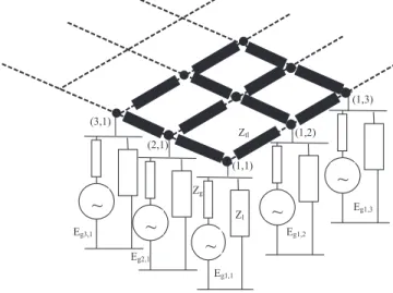
Fig. 1. Power system benchmark. The transmission network is a grid of
dimensionsn × n.
with respect to their ability to assess whether at least one machine is going to lose synchronism. As a matter of fact, most of the computational refinements that were proposed during the last two decades to speed up these methods are intrinsically linked to the fact that once loss of synchronism of at least one generator can be ascertained, there is no reason to further check the dynamic response of the system, since it can be immediately declared as ‘unstable’. This is also true for other transient stability assessment methods proposed under the generic term of direct methods [7].
III. BUILDING THE CASE FOR STUDYING PROPAGATION RATHER THAT INCEPTION OF LOSS OF SYNCHRONISM
PHENOMENA
As said, transient stability phenomena have been studied for a long time in order to improve the dynamic response of power systems when subjected to large disturbances. This response was deemed to be satisfactory when all the machines remained in synchronism with each other after the disturbance [1]. This idea was reasonable when the power system was relatively small with respect to the size of individual power plants. Indeed, in such a context, the loss of synchronism of one machine (or one power plant) was equivalent to losing a significant percentage of power production and, consequently, was highly likely to jeopardizing the power system survival as a whole. As power systems become larger than before, and the use of smaller generation units (e.g, micro-turbines, gas/vapor turbines) becomes more and more widespread, it becomes less critical to ensure that every machine does not lose synchronism after the inception of plausible events. To illustrate these ideas we use the test power system shown in Figure 1. A similar power system has already been used in [8], [9] and [10] to study electromechanical wave propagation while here we focus on the propagation of some loss of synchronism instability mechanisms caused by large excursions of the machines’ angle and speed around their nominal values.
The schematic power system we use can be assimilated to an n × n grid. To each node is connected a generator
(through its internal reactance) and a load of the same size. The transmission lines connecting two adjacent nodes of the system are all identical. The main purpose of this section is to study the influence that the size of the grid (determined here by the parametern) and the size of generation units (determined here by the parameterp, with the larger p, the larger the output power of the unit) have on the loss of synchronism phenomena. The size of the generation unit is in our experiments also correlated to the loads’ impedances, the transmission lines’ impedances and the generators’ internal impedances.
The exact relations between the parameter p and these quantities are given in the Appendix. Roughly speaking, the larger n (for a fixed value of p) the more the power system can be assimilated to an intercontinental size system. The smaller p the more the power system can be assimilated to a system with microturbines being installed close to some local loads. The reader is referred to the Appendix in which the detailed description of this benchmark power system is presented including the mathematical equations describing its dynamics.
Unless explicitly stated otherwise, we will always consider that the simulation results have been generated using the following scenario: before t = 0, the system is in state (see the Appendix for a description of the steady-state conditions); at t = 0, a short-circuit is applied on the transmission line connecting bus (1,1) and bus (1,2); at t = 100 ms, the short-circuit is cleared by opening both ends of that line and the line is not reclosed afterwards during the period of analysis.
Notice that the generators are equipped with over(under)-speed protections which disconnect them from the grid when their speed deviates from more than +(-)10% of its nominal value.
A. Base case
The first power system model simulated has a relatively small number of machines, (n2= 25). The value of p is chosen
equal to 1 for this system.
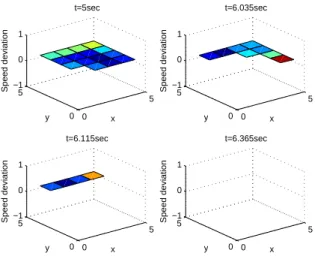
The results of the simulations are plotted on Figure 2. More precisely, this figure plots, at several instants, the value of the speed deviation of the generators. When a generator is disconnected from the network due to speed protection, the lines connecting the generator location to the rest of the system are not shown anymore on the graphic.
As one can see on Figure 2, the instability mechanism propagates from the fault location towards the entire network in a faster and faster way, and, at t = 6.365 seconds, all the machines have been disconnected from the system by their overspeed protections.
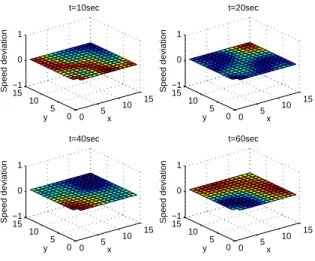
B. Evaluating the impact of system interconnection growth
The second power system studied has more machines than the first one (n = 10 rather than n = 5) and the value of p is kept unchanged. Similarly to what was observed previously, the instability mechanism also propagates to the whole system (see Figure 3). However, the loss of all machines is only observed now after 35.195 seconds. If n is increased
0 5 0 5 −1 0 1 x t=5sec y Speed deviation 0 5 0 5 −1 0 1 x t=6.035sec y Speed deviation 0 5 0 5 −1 0 1 x t=6.115sec y Speed deviation 0 5 0 5 −1 0 1 Speed deviation t=6.365sec x y
Fig. 2. Propagation of loss of synchronism for a5 × 5 grid (all generators
are lost aftert = 6.365s).
0 5 10 0 5 10 −1 0 1 x t=10sec y Speed deviation 0 5 10 0 5 10 −1 0 1 x t=34.6sec y Speed deviation 0 5 10 0 5 10 −1 0 1 x t=34.67sec y Speed deviation 0 5 10 0 5 10 −1 0 1 Speed deviation t=35.195sec x y
Fig. 3. Propagation of loss of synchronism for a10 × 10 grid (all generators
are lost aftert = 35.195s).
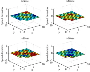
to 15, and p is still kept equal to 1, we observe that the loss of synchronism does not propagate anymore to the whole system. Only a handful of machines are lost in the post fault configuration, as illustrated by Figure 4.
Figure 5 shows, for various numbers n2 of machines in
the power system (with p always equal to 1), the log of the percentage of generation lost after 10 seconds. As one can see, whenn2 increases, the percentage of machines lost tends
to decrease and even reaches almost zero for a very large system. We draw three main conclusions from this first set of experiments. First, there is really a phenomenon of spatial propagation of the loss of synchronism phenomena throughout the system. Second, this propagation takes more time to spread to the whole system when its geographical size increases. Third, the instability mechanism can even naturally contain itself in its early stages when the system is large enough.
0 5 10 15 0 5 10 15 −1 0 1 x t=10sec y Speed deviation 0 5 10 15 0 5 10 15 −1 0 1 x t=20sec y Speed deviation 0 5 10 15 0 5 10 15 −1 0 1 x t=40sec y Speed deviation 0 5 10 15 0 5 10 15 −1 0 1 x t=60sec y Speed deviation
Fig. 4. Propagation of loss of synchronism for a15 × 15 grid.
0 100 200 300 400 500 600 700 −1 −0.5 0 0.5 1 1.5 2
number of identical units
log(% of generators lost at 10 sec)
Fig. 5. Influence of the size (n2) of the power system on the amount of
generation lost after10 seconds.
C. Evaluating the impact of dispersion
Up to now, we have illustrated the influence of the size of the power system on its instability mechanisms. Now we want to study what is the influence on the stability of the system of having many small machines rather than a few big ones.
To do so, we will increase the number of units (by increasing the value of n) while decreasing at the same time the power production capacity of each unit in a way that the total power production of the system is kept constant. We do this by adjustingp at the same time as n so as to keep p×n2constant
(i.e. p ∝ n−2).
In this experiment, the machine and network parameters are adapted so as to ensure that the small capacity units supposed to replace a large capacity unit can somehow be seen as equivalent (on an electrical and mechanical point of view) to this large unit (see the Appendix). Notice that the parameters of the lines are adapted to the value of p so that the electrical distance between two geographically adjacent points of the power system remain roughly the same when the generation
0 5 0 5 −1 0 1 x t=5sec y Speed deviation 0 5 0 5 −1 0 1 x t=10.7sec y Speed deviation 0 5 0 5 −1 0 1 x t=10.75sec y Speed deviation 0 5 0 5 −1 0 1 Speed deviation t=11.6sec x y
Fig. 6. Propagation of loss of synchronism for a network withn = 5 and
p = 1.5 (all generators are disconnected after t = 11.6s).
0 5 0 5 −1 0 1 x t=5sec y Speed deviation 0 5 0 5 −1 0 1 x t=13.085sec y Speed deviation 0 5 0 5 −1 0 1 x t=13.14sec y Speed deviation 0 5 0 5 −1 0 1 x t=13.25sec y Speed deviation
Fig. 7. Propagation of loss of synchronism for a network withn = 9 and
p = (25/81) ∗ 1.5 (all generators are disconnected after t = 13.25s).
system becomes more dispersed.1
To study the impact of smaller machines rather than big ones on the stability of the system, three simulations of the power system have been done. For the first simulation, the value of n has been chosen equal to 5 and the value of p to 1.5. The system response is shown in Figure 6. All the machines are lost after11.6 seconds.
For the second simulation, n is changed to 9 and p is changed to (25/81) ∗ 1.5. The system response is shown in Figure 7.
The third simulation (see Figure 8) is carried out for a value ofn equal to 11 and a value of p equal to (25/121) ∗ 1.5.
By putting Figure 6, 7 and 8 in perspective, we can conclude that when the machines become smaller (and for a fixed amount of total power production), the propagation of the loss
1Here we do not study as previously an increase of the geographical size
of the power system but well of the appearance of smaller generation units.
Therefore, a larger value ofn corresponds here to a finer transmission grid
0 5 10 0 5 10 −1 0 1 x t=10sec y Speed deviation 0 5 10 0 5 10 −1 0 1 x t=20sec y Speed deviation 0 5 10 0 5 10 −1 0 1 x t=40sec y Speed deviation 0 5 10 0 5 10 −1 0 1 x t=60sec y Speed deviation
Fig. 8. Propagation of loss of synchronism for a network withn = 11 and
p = (25/121) ∗ 1.5.
of synchronism phenomena to the whole system takes more time and that it is even naturally stopped if the machines are small enough.
IV. COUNTERACTING THE PROPAGATION OF LOSS OF SYNCHRONISM
To mitigate, in the aftermath of a contingency, the risk of blackout due to some loss of synchronism phenomena, two main types of strategies can be adopted. The first one can be assimilated to a preventive control strategy which amounts to operate the system with security margins which are high enough to decrease the likelihood of any initial loss of synchronism in case of large disturbances. The second one consists of implementing emergency control strategies which take in the aftermath of a severe contingency appropriate actions to lessen any potential effect of such a loss of synchro-nism. Both preventive and emergency control schemes have already been proposed for transient stability [2], [6]. However, these schemes have never really exploited (at least explicitly), the progressive spatial propagation of the loss of synchronism phenomena that was illustrated in previous section. In this section, we briefly describe a kind of emergency control scheme which exploits this spatial propagation.
The scheme is based on a system islanding strategy and is schematically described in Figure 9; it is an extension of already published ideas about controlled islanding schemes [11], [12]. This scheme works as follows. Once the power system is considered as being at risk of developing wide-spread instability mechanisms, the emergency control scheme is put on an alert state and the system is closely monitored to check whether some loss of synchronism phenomena propa-gate through the system or not. If such phenomena are indeed found to propagate to the system, the instability propagation mechanism is identified and a well chosen set of lines sur-rounding the area from which the instability propagates are opened in a coordinated manner so as to isolate the origin of the problem. While, in principle, the scheme is simple,
Fig. 9. Emergency control scheme for stopping the propagation of the loss
of synchronism phenomena. 0 5 10 0 5 10 −1 0 1 x t=5sec y Speed deviation 0 5 10 0 5 10 −1 0 1 x t=10sec y Speed deviation 0 5 10 0 5 10 −1 0 1 x t=20sec y Speed deviation 0 5 10 0 5 10 −1 0 1 x t=60sec y Speed deviation
Fig. 10. Propagation of loss of synchronism in the10 × 10 grid equipped
with an islanding scheme.
its implementation on a real-life power system would how-ever require answering show-everal non-trivial technical questions. Among them, one can mention for example those related to the non-negligible times needed for gathering the appropriate information from the power system, computing the appropriate actions and effectively applying them to the system. It is also expected that the sudden islanding of a zone of the system may also create new types of instability mechanisms (e.g., imbalance between production and generation) that could also lead to a significant blackout of the system.
As a way to illustrate the benefits in terms of stability that an islanding strategy can potentially bring, we have run a simulation on the benchmark power system (withn = 10 and p = 1) by considering the same contingency as before but this time by using an islanding based emergency control scheme. When no islanding scheme was used, the machine connected at node(1, 1) was first lost and the instability mechanism was found propagating afterwards to the whole system (see Figure 3). The islanding control scheme opens the transmission lines surrounding the zone composed of the four buses(1, 1), (1, 2), (2, 2) and (2, 1) a few instants after the machine connected to the node (1, 1) is disconnected from the system. The results are plotted in Figure 10. As one can observe, the opening of
these transmission lines indeed stops the propagation of the loss of stability.
V. CONCLUSIONS
We have illustrated through some simulations carried out on an academic test system that analyzing transient stabil-ity phenomena by declaring instabilstabil-ity once some (or one) machines were losing stability could be limitative. Indeed, we found out that when the test power system was growing in size and/or when the size of the generation units was decreasing, these instability phenomena could stay local and only jeopardizing in a marginal way the integrity of the whole system. Additionally, we found out that even if a significant percentage of the machines or all of them go out of step in the aftermath of a dangerous contingency, the spatial propagation of the instability could be exploited to design islanding-based emergency control schemes.
While there are many assumptions behind the power system upon which these findings were made (e.g., ”regularity” of the test system, simple model adopted to represent the machines’ dynamics), we believe that they may however question whether new types of analysis/control tools that look beyond the classical transient stability boundary of a power system should not be developed. For more than fifty years now most of the work in the field has exploited (more or less closely) the concept of Lyapunov’s second method developed to analyze the stability of non-linear systems [3]. While system theory was still in its infancy − and even not existing as a research field in itself − when transient stability phenomena were first described, this research community is now vibrant. Therefore, it would be interesting to investigate whether some other sta-bility paradigms would not be more adapted than the Lyapunov one to study transient stability phenomena. Also, it could be interesting to formalize, at a higher level of abstraction than the one adopted in this paper, the problem of transient stability when one allows a portion of machines to go out of step, and to develop some generic system analysis tools that could also be used for some other applications (e.g., cascading failures related to over-current protection of transmission lines).
APPENDIX
We provide in this appendix a detailed description of the benchmark power system sketched on Figure 1. This bench-mark power system depends on two main parameters: n and p. Roughly speaking, the parameter n determines the ’size’ of the network (when n increases −and for a given value of p − the power system can be seen as growing geographically while keeping the same generation and transmission structure) while the parameter p is correlated to the type of generation and to the transmission structure (the smaller p, the more the power system can be assimilated to a power system with small generation units located close to the loads).
The transmission grid of this system can be seen as an × n regular grid. A line connecting two adjacent buses of this grid has been modelled by using the reactanceZtl= √p ∗ j0.1 pu.
To every node of this grid is connected in parallel a generator and a load. All the loads are modelled using the following reactanceZl= 1p∗ (0.8 + j0.6) pu.
The generators are also considered as being identical. To represent the electrical part of the generators, the classical constant-voltage-behind reactance model has been adopted. The internal reactanceZgof a generator is equal to 1p∗j0.01 pu and the magnitude of its internal voltage is chosen equal to 1 pu.
The mechanical dynamics of a generator is modelled by using the following differential equations:
Mdω
dt + ωrDω = Pm− Pe (1)
dδ
dt = ω − ωr (2)
where ωr = 1 pu is the reference angular frequency (the
angular frequency of the synchronous rotating axis) of the generator,D = p ∗ 0.007 pu is the damping constant, M = p ∗ 0.3 pu its inertia constant, Pm= p ∗ 0.7904 pu its mechanical
power, Pe its electrical power, δ its rotor angle and ω its
angular frequency. The electrical power Pe of the machine,
its angleδ and its speed ω vary with time.
As initial steady-state conditions for this system, we have always considered in our simulations the state for which all the generators have the same rotor angle, a situation which corresponds to the case where there is initially no current going through the transmission lines.
REFERENCES
[1] P. Kundur, J. Paserba, V. Ajjarapu, G. Andersson, A. Bose, C. Canizares, N. Hatziargyriou, D. Hill, A. Stankovic, C. Taylor, T. Van Cutsem, and V. Vittal, “Definition and classification of power system stability,” IEEE
Transactions on Power Systems, vol. 19, no. 3, pp. 1387–1401, August
2004.
[2] L. Wehenkel, “Emergency control and its strategies,” in Proceedings of
the 13th Power Systems Computation Conference, PSCC99, June 1999,
pp. 35–48.
[3] D. Pavella, M. Ernst and D. Ruiz-Vega, Transient Stability of Power
System A unified Approach to Assessment and Control. Kluwer Academic Publishers, 2000.
[4] M. Begovic, G. Jean-Marie, G. Paulo, W. Lachs, C.-C. Liu, V. Madani, D. Novosel, G. Trudel, M. Amin, H. Clark, I. Dobson, P. Donalek, P. Grondin, and L. Wehenkel, “Defense plan against extreme contingen-cies - CIGRE TF C2.02.24 - Summary for Electra,” Electra, no. 231, pp. 46–61, April 2007.
[5] P. Kundur, Power System Stability and Control. McGraw-Hill, 1994.
[6] L. Wehenkel and M. Pavella, “Preventive vs emergency control of power systems,” in Proc. of IEEE PES Power System Conference and
Exposition (PSCE-2004), vol. 2, October 2004, pp. 1665 – 1670.
[7] M. A. Pai, Energy Function Analysis for Power System Stability, ser.
Power Electronics and Power Systems. Kluwer Academic Publishers,
1989.
[8] J. S. Thorp, C. E. Seyler, and A. G. Phadke, “Electromechanical wave propagation in large electric power systems,” IEEE Transactions on
Circuits and Systems I: Fundamental Theory and Applications, vol. 45,
no. 6, pp. 614–622, June 1998.
[9] J. S. Thorp, C. E. Seyler, M. Parashar, and A. G. Phadke, “The large scale electric power system as a distributed continuum,” IEEE Power
Engineering Review, vol. 18, no. 1, pp. 49–50, January 1998.
[10] L. Huang, M. Parashar, A. Phadke, and J. Thorp, “Impact of electrome-chanical wave propagation on power system protection and control,”
CIGRE Paris, France, no. 34, pp. 201–206, August 2002.
[11] S. Ahmed, N. Sarker, A. Khairuddin, M. Ghani, and H. Ahmad, “A scheme for controlled islanding to prevent subsequent blackout,” IEEE
Transactions on Power Systems, vol. 18, no. 1, pp. 136–143, February
2003.
[12] B. Yang, V. Vittal, and G. Heydt, “Slow-coherency-based controlled islanding - A demonstration of the approach on the August 14, 2003 blackout scenario,” IEEE Transactions on Power Systems, vol. 21, no. 4, pp. 1840–1847, November 2006.