Vol. 00, No. 00, 00 Month 20XX, 1–17
The Use of Time Series Forecasting in Zone Order Picking Systems to Predict Order Pickers’ Workload
Teun van Gilsa∗, Katrien Ramaekersa, An Carisa, and Mario Coolsb
aResearch Group Logistics, Hasselt University, Agoralaan Building D, 3590 Diepenbeek, Belgium; bDepartment ARGENCO, Local Environment Management & Analysis, Universit´e de Li`ege, All´ee de la
D´ecouverte 9, Quartier Polytech 1, 4000 Li`ege, Belgium
(October 2015)
In order to differentiate from competitors in terms of customer service, warehouses accept late orders while providing delivery in a quick and timely way. This trend leads to a reduced time to pick an order. This paper introduces workload forecasting in a warehouse context, in particular a zone picking warehouse. Improved workforce planning can contribute to an effective and efficient order picking process. Most order picking publications treat demand as known in advance. As warehouses accept late orders, the assumption of a constant given demand is questioned in this paper. The objective of this study is to present time series forecasting models that perform well in a zone picking warehouse. A real-life case study demonstrates the value of applying time series forecasting models to forecast the daily number of order lines. The forecast of order lines, along with order pickers’ productivity, can be used by warehouse supervisors to determine the daily required number of order pickers, as well as the allocation of order pickers across warehouse zones. Time series are applied on an aggregated level, as well as on a disaggregated zone level. Both bottom-up and top-down approaches are evaluated in order to find the best performing forecasting method.
Keywords: case study; operations planning; order picking management; forecasting; workload balancing
1. Introduction
As customer markets globalize, supply chains increasingly depend on efficient and effective logistical systems in order to distribute products in a large geographical area. A warehouse can be defined as a facility where activities of receiving, storing, order picking, and shipping are performed. Warehouses are an important part of supply chains, and therefore warehouse operations need to work in an efficient and effective way (Gu, Goetschalckx, and McGinnis 2007).
Warehouses are generally confronted with highly seasonal demand patterns. The primary tool in coping with demand fluctuations is the labour force. Temporary workers are often hired in order to capture the workload peaks. Forecasting the daily warehouse demand is a key issue in controlling the amount of staff (De Koster, Le-Duc, and Roodbergen 2007; Ruben and Jacobs 1999). Because order picking is recognized as the most crucial warehouse operation, this paper focuses on forecasting order pickers’ workload in order to control the number of order pickers. Workload forecasting can be defined as predicting the future amount of work to be performed in order to meet demand. The forecast workload can be translated into a required number of order pickers depending on order pickers’ productivity. On the one hand, an insufficient number of available order pickers reduces the service level. On the other hand, planning too many order pickers causes unnecessarily high labour costs.
A large number of workforce related studies have been conducted in manufacturing environments,
but similar studies in warehouses are rather limited (Davarzani and Norrman 2015). The strongly daily fluctuating demand, which requires maximum flexibility, differentiates warehouses from man-ufacturing environments. Warehouses deliver labour-intensive services to customers. Personnel ca-pacity drives the service quality to customers and resulting warehouse performance. Forecasting the workload and scheduling workers are the main tools to guarantee order fulfilment operations in a timely way (Sanders and Ritzman 2004; Defraeye and Van Nieuwenhuyse 2016).
The main focus in the literature is on warehouse design and individual warehouse processes. These topics have recently been reviewed by Davarzani and Norrman (2015), De Koster, Le-Duc, and Roodbergen (2007), Gu, Goetschalckx, and McGinnis (2007), Gu, Goetschalckx, and McGinnis (2010), and Rouwenhorst et al. (2000). Among these literature reviews, De Koster, Le-Duc, and Roodbergen (2007) specifically focus on manual order picking processes, as the large majority of order picking operations in warehouses are performed manually. According to De Koster, Le-Duc, and Roodbergen (2007), manual order picking systems account for 80% of all order picking systems in Western Europe. Whether the order picking process is done manually or automatically, high costs are related to this process (Gu, Goetschalckx, and McGinnis 2007). Order picking as a warehouse function arises because goods are received in large volumes, and customers order small volumes of different products. In other words, customers can order products from a great variety of suppliers. Each customer order is composed of one or more order lines, with every order line representing a single stock keeping unit (SKU) (De Koster, Le-Duc, and Roodbergen 2007).
Order picking management, in particular organizing efficient and flexible systems to retrieve SKUs from the warehouse, has been identified as an important and complex operation. In order to differentiate from competitors in terms of customer service, warehouses accept late orders from customers while providing delivery in a quick and timely way. By accepting late orders, the time remaining to pick an order is reduced. Furthermore, the order behaviour of customers has changed from ordering few and large orders to many orders consisting of only a limited number of order lines (De Koster, Le-Duc, and Roodbergen 2007). The changed order behaviour is amplified by the delivery of e-commerce markets and forces warehouses to handle a larger number of orders, while order picking time has shortened.
One way of moving to a more efficient order picking process is dividing a warehouse into different smaller areas, or order picking zones. Each order picking zone is dedicated to a few order pickers. As a consequence, each order picker travels in a pre-specified part of the warehouse, and thus travel time is reduced. Furthermore, order pickers become familiar with the item locations in the zone. Besides the efficiency benefits resulting from the division of the warehouse into several order picking zones, two disadvantages are linked to zone picking: orders are split and must be consolidated again before shipment, and labour resources should be allocated across all order picking zones. Either progressive zoning or synchronized picking is used to deal with the first disadvantage. In progressive zoning, orders are picked zone by zone. Synchronized zoning refers to the policy where all order pickers can work on the same order at the same time, each order picker in his own zone. After picking, all orders are consolidated through a sorting system (De Koster, Le-Duc, and Roodbergen 2007).
This paper focusses on opportunities to deal with the second disadvantage of zone picking. By fulfilling customer orders in a quick and timely way, space, labour, and equipment resources should be allocated across all order picking zones (Gu, Goetschalckx, and McGinnis 2007). Moreover, a flexible workforce planning is required to allocate the order pickers across warehouse zones. For example, order pickers can be transferred to different pick zones, which results in the necessity to cross-train workers. Furthermore, the moment of transferring a cross-trained worker to another zone should be established, as well as to which new order picking zone a worker should be as-signed. Thus, reliable and accurate forecasting is required to support warehouse supervisors in determining the daily required number of order pickers, as well as in allocating the order pickers across zones. This paper concentrates on the first step of personnel capacity planning, in particular forecasting the workload based on empirical data. The three other steps introduced by Defraeye
and Van Nieuwenhuyse (2016) (i.e., determining staffing requirements, shift scheduling, and shift assignment) are beyond the scope of this paper.
To the best of our knowledge, we are the first to forecast order pickers’ workload in a warehouse. Most order picking publications treat demand as known in advance (De Koster, Le-Duc, and Roodbergen 2007; De Koster, Le-Duc, and Zaerpour 2012; Hwang and Kim 2005). As warehouses accept late orders, the assumption of a constant given demand should be reconsidered. Based on real demand data, Jane (2000) and Jane and Laih (2005) balance the workload by analysing different zone sizes in a progressive zone picking warehouse and different assignments of products to order picking zones in a synchronized zone picking warehouse, respectively. These approaches are expected to balance the workload among zones in the long term. Dynamic zone picking systems, such as bucket brigades, can be used to solve the balancing problems in the short term. Bucket brigades are flexible order picking systems and self-balancing with respect to the workload of order pickers. However, bucket brigades can result in efficiency losses and assume that the picking area is divided into several serial zones (Koo 2008). Another approach to balance order pickers’ workload among order pickers in the short term is to forecast the workload. Reliable daily forecasts can be used to schedule order pickers. For daily planning purposes, the total number of order lines, as well as the distribution of these aggregated order lines across the different order picking zones, are required to determine the required number of order pickers as well as to allocate the order pickers across zones. The forecasting approach is not restricted to serial zone picking systems, which can result in buffers, as orders should be consolidated.
The objective of this study is to present forecasting methods, especially time series models, that perform well in a zone picking warehouse, in particular in forecasting the number of order lines. A real-life case study demonstrates the value of applying time series forecasting models to the warehouse demand. This paper provides forecasting methods able to accurately and reliably predict the next-day workload of an international warehouse. Moreover, two different forecasting approaches, including top-down forecasting and bottom-up forecasting, are tested in order to pro-vide accurate aggregated forecasts as well as accurate forecasts at zone level. Forecasts at different levels of aggregation are required to help warehouse supervisors schedule the order pickers on a daily basis.
The gap between academic research and practice (Davarzani and Norrman 2015; De Koster, Le-Duc, and Roodbergen 2007; Gu, Goetschalckx, and McGinnis 2007), as well as the fact that almost all research in order picking treats demand as given (De Koster, Le-Duc, and Roodbergen 2007) and ignores the determination of the number of personnel (Rouwenhorst et al. 2000), are com-mon conclusions in recent literature reviews on warehouse planning. These previously determined research gaps are filled in this study. The main contribution of this study is to present a proof of concept of forecasting methods in a warehouse context, especially a zone picking warehouse, in order to efficiently and effectively manage order picking activities. The case study provides manage-rial insights into the impact of forecasting on planning order pickers in a warehouse. A preliminary version of this paper was presented at the 27th European Conference on Operational Research (Van Gils et al. 2015).
The remainder of the paper is organized as follows: the next section (section 2) introduces the case study. Section 3 outlines the research methodology used in this study, followed by the empirical results of the real-life case in section 4. Section 5 is devoted to the concluding remarks and future research directions.
2. Description Case Study
The case of this study is based on a large international warehouse located in Belgium. The ware-house, which stores and delivers automotive spare parts to delivery points all over the world, is a fully manually operated warehouse. This conventional handling results in fast, frequent, and reliable
deliveries. The warehouse focusses on distributing products in order to provide customers first-class service that contributes to a maximum operating time for their vehicles. For example, customers expect certain order types, especially spare parts for vehicles off road, to have a throughput time of only two hours in order to minimize the downtime. Determining the daily required number of human resources in order to provide the high customer service level is perceived as a complicated task by warehouse supervisors. As customers are allowed to order two hours before the shipping deadline, forecasting is required to determine the daily required number of order pickers.
The daily number of order lines of the warehouse is used to estimate and evaluate different time series forecasting methods. The forecasts of order lines, along with order pickers’ productivity, are used by the warehouse supervisors to determine the daily required number of order pickers in order to provide a high customer service level. Supervisors are currently forecasting the total daily number of order lines. These forecasts are based on experience and personal judgment, without using forecasting models. The supervisors’ forecasts are used as benchmarks for evaluating the proposed time series forecasting models in this paper. The objective of the case study is to find time series that are able to produce more reliable forecasts compared to current non-statistical forecasts, making the workforce planning less dependent on the availability of experienced supervisors.
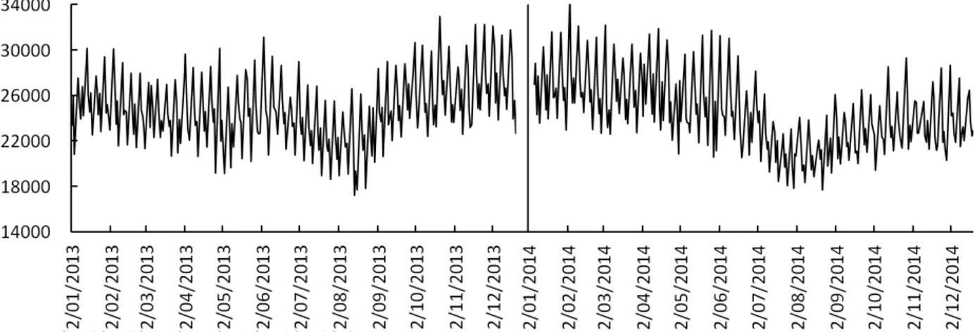
Order lines for the years 2013 and 2014 are considered. The demand of 2013 is used to estimate model coefficients, and the order lines of 2014 are used as out-of-sample values. This method of ex post forecasting is applied to validate the proposed forecasting models. In figure 1, the real daily number of order lines for the years 2013 and 2014 is plotted, in particular the accumulated daily number of order lines of each order picking zone. For both years, order lines strongly fluctuate.
Figure 1. Real daily number of order lines.
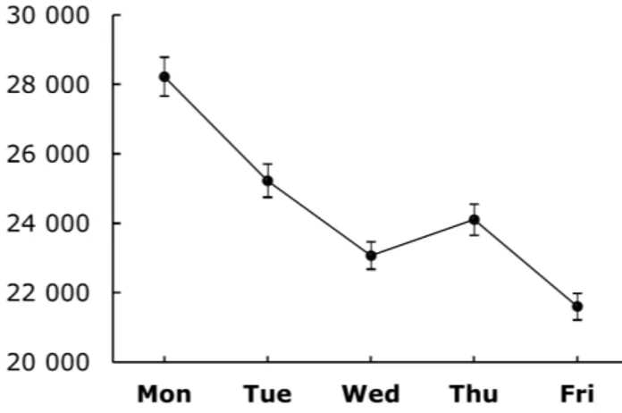
In order to gain prior insight into the potential seasonal cycles in the daily number of order lines, a spectral analysis is performed. A spectral analysis is a statistical method to detect regular cyclical patterns. The reader is referred to Cools, Moons, and Wets (2009) for a more extensive description of a spectral analysis. By looking at the results of the spectral analysis presented in figure 2, both a semi-weekly and weekly recurring cycle can be identified in the data as indicated by respectively the global maximum at period 2.5 and the local maximum at period 5. The global maximum also contributes to an explanation of the weekly cyclical pattern, as repetition of these patterns also yields a weekly pattern. The weekly recurring cycle is shown in figure 3. On average, the number of order lines is high on Mondays and decreases all other days of the week, except on Thursdays. The curve shows a significant rise on Thursdays, as illustrated by the narrow, non-overlapping 95% confidence intervals in figure 3. Additionally, a Bonferroni test is performed to compare the mean values. The test demonstrates a statistically significant difference between the number of order lines for every pair of working days, using 0.01 as the critical significance level.
Figure 2. Spectral analysis for aggregated daily number of order lines.
Figure 3. Mean and 95% confidence intervals illustrating the weekly seasonal cycle.
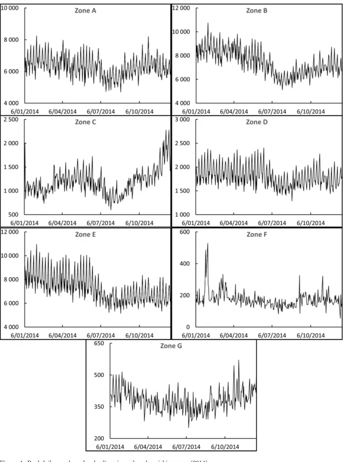
The studied warehouse is divided into seven different order picking zones, named zone A to zone G. Figure 4 depicts the real number of order lines in each order picking zone for the year 2014. In terms of order line volume, three large order picking zones (i.e., zones A, B, and E) can be distinguished. Furthermore, the warehouse consists of two middle-sized zones (i.e., zones C and D) and two rather small ones (i.e., zones F and G). Order line data for zones A, B, D, and E show a similar weekly seasonal cycle as shown in figure 3. This seasonal pattern is less clear in the other order picking zones.
Dividing the warehouse into order picking zones implies that all order pickers should be dis-tributed across the different order picking zones. A synchronized zone picking policy is employed in the warehouse under consideration in order to retrieve a large number of orders in short time windows. Because of the efficiency benefits resulting from synchronized zone picking, this zone picking policy is commonly employed in warehouses (Le-Duc and De Koster 2005) and is especially useful in serving e-commerce markets. Furthermore, the proposed forecasting techniques can be generalized to progressive zoning in order to provide insights into the workload, as balancing the workload over order pickers is an important issue in progressive zoning, as well (Jane 2000; Jane and Laih 2005).
Because disaggregated forecasts are currently lacking, allocating order pickers across zones is perceived as a hard activity by supervisors. Therefore, hierarchical forecasting is introduced in the zone picking warehouse. Hierarchical forecasting refers to the problem of identifying a level of
Figure 4. Real daily number of order lines in each order picking zone (2014).
forecasting aggregation that provides adequate information for decision making. Forecasting can be done on an aggregated as well as a disaggregated level. A top-down forecasting process uses aggregate demand data to forecast total demand, after which individual forecasts can be derived from the aggregated forecast. In the bottom-up approach, demand is forecast for each individual demand segment. Subsequently, these forecasts are accumulated to produce an aggregated forecast (Schwarzkopf, Tersine, and Morris 1988; Song and Li 2008; Zotteri, Kalchschmidt, and Caniato 2005).
In a warehouse context, demand forecasting on aggregate data is relevant for determining the daily total number of order pickers required to fulfil all customer orders, while forecasting the number of order lines at a disaggregate level will additionally help supervisors allocate the order pickers across all warehousing zones. The different disaggregated demand segments in a warehouse are defined by the daily order lines of each order picking zone.
Both aggregated and disaggregated forecasts are required for flexible workforce scheduling. The flexible workforce scheduling problem in a zone picking warehouse includes the distribution of order pickers across different order picking zones, when a cross-trained worker should be transferred to another zone and to which new order picking zone a worker should be assigned.
3. Forecasting Models and Accuracy Measures
This section outlines the mathematical and theoretical framework of different time series forecasting methods. Time series forecasting is considered as an important forecasting area, where a variable is explained with regard to its own historical observations and a random error term. Time series are able to recognize historical trends and patterns and extrapolate these trends into the future (Song and Li 2008). De Gooijer and Hyndman (2006) give an overview of past research in the area of time series forecasting. Methods like exponential smoothing and different variants of SARIMA are extensively discussed by De Gooijer and Hyndman (2006). Gardner Jr. (2006) specifically focuses on exponential smoothing forecasting models and presents state of the art research on exponential smoothing. Time series forecasting has been extensively used in areas other than warehousing, such as urban water consumption (House-Peters and Chang 2011) and energy consumption (Suganthi and Samuel 2012). Moreover, the application of time series forecasting to tourism demand is the most extensively studied forecasting practice (Athanasopoulos et al. 2011; Song and Li 2008).
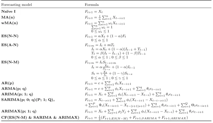
This article analyses and applies twelve different forecasting models to the order line data in the case study. The major difference among these methods is the way trends and seasonal patterns are treated. Time series forecasting models are classified into different categories, in particular the Na¨ıve method, moving average methods, exponential smoothing models, SARIMA forecasting models, and finally composite forecasting, in which different previous defined models are combined. The mathematical representations of the forecasting methods are summarized in table 1. All forecasting methods are briefly outlined in this section. More elaborated time series forecasting discussions can be found in Chase Jr (2013) and De Gooijer and Hyndman (2006).
The first method, Na¨ıve I, is the most straightforward forecasting method. Potentially existing trends and seasonal patterns in the data are neglected. The na¨ıve method can be extended by taking multiple historical periods into account. The simple moving average model (M A(n)) averages n previously observed values. By averaging multiple periods, more historical information is considered in the forecasting value. By giving equal weight to each historical value, the simple moving average model assumes neither trend nor seasonality (Goh and Law 2002; Song and Li 2008). Seasonality can be incorporated into a moving average model by allowing each component to have a different weight, ωi, in the moving average equation. Large weights are an indication of highly influential observations in the forecasting value. This forecasting method is known as a weighted moving average model (wM A(n))(Jacobs, Chase, and Chase 2010).
histor-Table 1. Summary of time series forecasting models.
Forecasting model Formula
Na¨ıve I Ft+1= Xt
MA(n) Ft+1=n1Pni=1Xt−i+1
wMA(n) Ft+1=Pni=1ωiXt−i+1
Pn i=1ωi= 1 0 ≤ ωi≤ 1 ES(N-N) Ft+1= αXt+ (1 − α)Ft 0 ≤ α ≤ 1 ES(A-N) Ft+m= It+ mTt It= αXt+ (1 − α)(It−1+ Tt−1) Tt= β(It− It−1) + (1 − β)Tt−1 0 ≤ α ≤ 1 ; 0 ≤ β ≤ 1 ES(N-M) Ft+m= ItSt−s+m It= αSXt t−s + (1 − α)It−1 St= γXIt t + (1 − γ)St−s 0 ≤ α ≤ 1 ; 0 ≤ γ ≤ 1
AR(p) Ft+1= c +Ppi=1φiXt−i+1
ARMA(p; q) Ft+1= c +Ppi=1φiXt−i+1+Pqi=1θiet−i+1
ARIMA(p; 1; q) Ft+1= Xt+Ppi=1φi(Xt−i+1− Xt−i) +
Pq
i=1θiet−i+1
SARIMA(p; 0; q)(P; 1; Q)s Ft+1= Xt−s+1+Ppi=1φi(Xt−i+1− Xt−i−s+1)
+PP
i=1Φi(Xt−is+1− Xt−(i+1)s+1) +
Pq
i=1θiet−i+1+PQi=1Θiet−is+1
ARIMAX(p; 1; q) Ft+1= Xt+P4j=1ρjYj+
Pp
i=1φi(Xt−i+1− Xt−i) +
Pq
i=1θiet−i+1
CF(ES(N-M) & SARIMA & ARIMAX) Ft+1=13(Ft+1;ES(N −M )+ Ft+1;SARIM A+ Ft+1;ARIM AX)
c = regression constant
d = order of nonseasonal differencing D = order of seasonal differencing et= forecasting error in the current period
Ft= forecasting value in the current period
Ft+1= forecasting value in period t + 1
It= smoothed level of the series in the current period
j = working day (1 = Monday; 2 = Tuesday; 3 = Wednesday; 4 = Thursday) m = number of periods ahead to be forecast
n = number of historical periods averaged
p = number of nonseasonal autoregressive components P = number of seasonal autoregressive components q = number of nonseasonal moving average components Q = number of seasonal moving average components s = number of periods in one seasonal cycle St= smoothed seasonal index in the current period
t = period
Tt = smoothed additive trend in the current period
Xt= observed value in the current period
Yj = binary working day variable
α = smoothing parameter for the level of the time series β = smoothing parameter for the trend
γ = smoothing parameter for the seasonal indices θ = nonseasonal moving average parameters Θ = seasonal moving average parameters ρ = working day regression parameters φ = nonseasonal autoregression parameters Φ = seasonal autoregression parameters ω = weight
ical values are averaged. In contrast to the above described moving average models, the averaging of historical values is done in an exponential way. In other words, the weights in the forecasting model drop exponentially for older values. Various exponential smoothing models can be distin-guished based on the way trends and seasonal patterns are considered. Three models are discussed in this paper, in particular simple exponential smoothing (ES(N-N)), Holt’s exponential smoothing (additive trend, no seasonality, ES(A-N)), and exponential smoothing considering a multiplicative seasonality (ES(N-M)) (De Gooijer and Hyndman 2006; Goh and Law 2002). The reader is referred to Gardner Jr. (2006) for an overview of other exponential smoothing methods.
Seasonal autoregressive integrated moving average models (SARIMA) exist in many different forms. The full formulation of a SARIM A(p, d, q)(P, D, Q)s model is given by:
φ(B)Φ(Bs)∇d∇Ds Xt+1= c + θ(B)Θ(Bs)et, (1) where:
c = regression constant; et = regression error term;
s = number of periods in one seasonal cycle; φ(B) = nonseasonal autoregressive operator; Φ(Bs) = seasonal autoregressive operator; θ(B) = nonseasonal moving average operator; Θ(Bs) = seasonal moving average operator; ∇d = nonseasonal dth differencing term; ∇D
s = seasonal Dth differencing at s number of lags.
Those operators will be only present in equation 1 in case the values p, P , d, D, q, and Q are different from zero (Cools, Moons, and Wets 2009). Four different SARIMA variants are outlined below.
Starting with the most straightforward SARIMA model where only p differs from zero, the SARIMA model is a pure autoregressive model (AR) of order p. The AR(p) forecasting model assumes that the forecasting value is only related to the p most recent historical values (Chase Jr 2013; Cools, Moons, and Wets 2009).
The simple AR(p) model can be extended by adding q moving average components. In the autoregressive moving average (ARMA) model, both p and q differ from zero. The forecasting value not only depends on its own past values, but also on q previous forecasting errors (Chase Jr 2013; Cools, Moons, and Wets 2009).
The major disadvantage linked to both AR(p) and ARM A(p, q) is the assumption of stationarity. Stationarity means that there is no trend in the data. The best way of eliminating a trend is by differencing the data, in particular taking the difference of observation t and observation t − 1. This model is known as an autoregressive integrated moving average (ARIMA) forecasting model. The forecasting value is calculated by the sum of last observation and a forecast shift compared to last period (Athanasopoulos et al. 2011; Chase Jr 2013; Cools, Moons, and Wets 2009).
While the ARIMA model is able to eliminate trends, the full SARIMA model, as represented by equation 1, is able to additionally take seasonal cycles into account. If seasonality exists in the data, seasonal differencing may be required. A seasonal difference is the difference between two corresponding observations from two consecutive seasonal cycles. The seasonal difference can be mathematically represented by Xt−i− Xt−i−s. By seasonal differencing, both trend and seasonal patterns can be eliminated at once. Therefore, the resulting time series may become stationary and require no further differencing (Athanasopoulos et al. 2011; Chase Jr 2013; Cools, Moons, and Wets 2009).
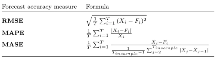
Table 2. Summary of forecast accuracy measures. Forecast accuracy measure Formula
RMSE q 1 T PT i=1(Xi− Fi)2 MAPE T1PT i=1 |Xi−Fi| Xi MASE T1PT i=1 Xi−Fi 1 Tinsample−1 PTinsample j=2 |Xj−Xj−1|
Fi= forecasting value in period i
i = time period
j = in-sample time period t = period
T = total number of forecast periods Ti= number of in-sample periods
Xi= observed value in period i
Y -variables is applied to the order line data. Four dummy variables are created to model the weekly seasonality. Those dummy variables represent the first four working days of the week (i.e., Monday, Tuesday, Wednesday, and Thursday). Friday is used as reference day to prevent multicollinearity (Cools, Moons, and Wets 2009).
SARIMA models are complex models to develop, as well as to use as forecasting method. How-ever, SARIMA models generally predict demand accurately in the short, medium, and long term due to the ability to account for both trends and seasonality (Chase Jr 2013).
Finally, composite forecasting (CF) describes methods of combining forecasting values of al-ternative forecasting models. By combining different forecasts, biases among methods compensate for one another. The strengths of each method are merged, resulting in better forecasting per-formances compared to individual forecasts. One method of composite forecasting applied in this paper is the simple averaging of several forecasting methods. Other composite forecasting models are described in Chase Jr (2013).
Improving forecast accuracy is of great importance in reducing uncertainty and meeting demand requirements (Sanders and Ritzman 2004). Many forecast accuracy measures have been used in past research. In order to evaluate the forecasting models, three different accuracy measures are used in this paper, namely root mean square error (RMSE), mean absolute percentage error (MAPE), and finally mean absolute scaled error (MASE). These three accuracy measures are mathematically represented in table 2. In Hyndman and Koehler (2006), more previously used measures of accuracy are discussed and compared.
The first proposed accuracy measure, RMSE, is a scale-dependent measure in comparing fore-casting methods. The main advantage of using RMSE as forefore-casting accuracy measure is the straightforward interpretation, as RMSE is on the same scale as the data. Because the forecast-ing objective is to minimize forecastforecast-ing error, a low value for RMSE is preferred (Hyndman and Koehler 2006).
MAPE is an accuracy measure based on percentage errors. MAPE is scale-independent and thus useful for comparing forecasting performance across different data sets. It has the disadvantage of having an extremely skewed distribution when any value of Xt is close to zero (Hyndman and Koehler 2006). MAPE has been identified as especially useful when units of measurement are relatively large (Goh and Law 2002). In the forecasting context a low value for MAPE is preferred, because a low value can be interpreted as a low percentage error. Because the daily number of order lines in a warehouse is different from zero and units of measurement are rather large, MAPE is a reliable forecasting accuracy measure.
A final accuracy measure proposed by Hyndman and Koehler (2006) is a scaled error. MASE
is independent of the data scale. If MASE has a value smaller than one, the proposed forecasting method gives, on average, smaller errors compared to the in-sample errors from the na¨ıve method. The na¨ıve method is thus used as benchmark in evaluating the forecasting accuracy by MASE (Hyndman and Koehler 2006).
4. Empirical Results
This section analyses and discusses the results of the study. In this paper, hierarchical forecasting is performed by applying both a bottom-up and a top-down approach to the order line data in the case study. Using the top-down forecasting process, first total daily number of order lines is forecast using time series forecasting models. Next, the zone-level forecast is derived from the aggregated forecast using a factor that defines the percentage of total number of order lines that should be picked in the order picking zone. For the bottom-up approach, the time series forecasting formulas are used to predict demand on zone level, after which these zone level forecasts are accumulated to derive aggregated demand.
This section is organized as follows: sections 4.1 and 4.2 present the results of the top-down forecasting process and the forecasting errors resulting from the bottom-up approach, respectively. Both forecasting approaches are statistically compared in section 4.3.
4.1 Top-down Forecasting Approach
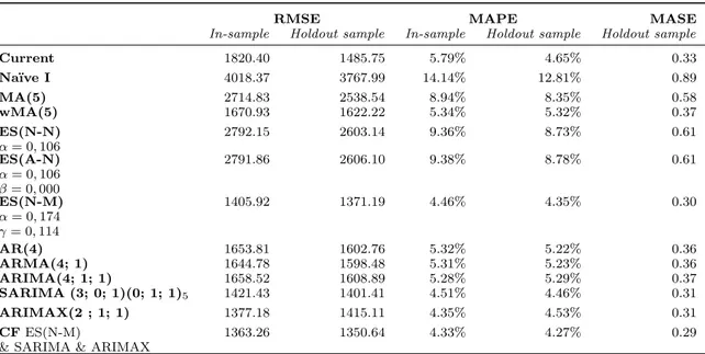
All twelve forecasting methods presented above are applied to the warehouse demand data. Results of the twelve forecasts, as well as the performance of non-statistical forecasts made by supervisors (Current) are presented in table 3. Coefficients of wMA(5), all exponential smoothing models and all variants of SARIMA are determined by minimizing the in-sample sum of squared residuals (SSR).
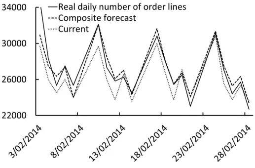
Figure 5. Current forecasts, composite forecasts, and the real daily number of order lines for the month February 2014. Results in table 3 show that all three forecasting accuracy measures are consistent in identi-fying the best performing forecasting method, both for in-sample forecasts and for out-of-sample
Table 3. Top-down approach: forecasting accuracy aggregated forecast.
RMSE MAPE MASE
In-sample Holdout sample In-sample Holdout sample Holdout sample
Current 1820.40 1485.75 5.79% 4.65% 0.33 Na¨ıve I 4018.37 3767.99 14.14% 12.81% 0.89 MA(5) 2714.83 2538.54 8.94% 8.35% 0.58 wMA(5) 1670.93 1622.22 5.34% 5.32% 0.37 ES(N-N) α = 0, 106 2792.15 2603.14 9.36% 8.73% 0.61 ES(A-N) α = 0, 106 β = 0, 000 2791.86 2606.10 9.38% 8.78% 0.61 ES(N-M) α = 0, 174 γ = 0, 114 1405.92 1371.19 4.46% 4.35% 0.30 AR(4) 1653.81 1602.76 5.32% 5.22% 0.36 ARMA(4; 1) 1644.78 1598.48 5.31% 5.23% 0.36 ARIMA(4; 1; 1) 1658.52 1608.89 5.28% 5.29% 0.37 SARIMA (3; 0; 1)(0; 1; 1)5 1421.43 1401.41 4.51% 4.46% 0.31 ARIMAX(2 ; 1; 1) 1377.18 1415.11 4.35% 4.53% 0.31 CF ES(N-M)
& SARIMA & ARIMAX
1363.26 1350.64 4.33% 4.27% 0.29
forecasts. The composite forecast of ES(N-M), SARIMA, and ARIMAX improves the current su-pervisors’ forecasts by 25.3% (1 −4.33%5.79%) and 8.2% (1 −4.27%4.65%) in terms of the in-sample MAPE and holdout-sample MAPE percentage reduction, respectively. Forecasting errors, both in-sample and out-of-sample, of ES(N-M), SARIMA(3; 0; 1)(0; 1; 1)5, as well as ARIMAX(2; 1; 1) are similar to the best performing CF. Neither other SARIMA variant nor the more simple forecasting models are able to accurately describe the seasonal cycles in the data; these models are not able to outperform current predictions done by supervisors. Figure 5 illustrates the forecasts, both Current and CF, as well as the real daily number of order lines. The figure is limited to the month of February 2014 because of visibility. However, other months are equivalent.
Besides demonstrating the best performing forecasting model, table 3 shows that almost all forecasting errors produced by the holdout sample are lower compared to the corresponding in-sample forecasting errors. Because supervisors were able to forecast more accurately during the year 2014, this observation seems to be caused by the nature of the data. Order lines seem to deviate less from the general pattern in 2014 compared to 2013.
A final remark on table 3 can be made concerning the results of ES(N-N) and ES(A-N). By including the trend component in the exponential smoothing model, only in-sample RMSE is slightly decreasing. All other forecasting errors have risen due to the inclusion of a trend component. This is in accordance with the observations on figure 1 that the trend is not significant.
Table 4 presents a more profound overview of the absolute scaled error (ASE). For each of the twelve forecasting models, the mean absolute scaled error, the standard deviation of the absolute scaled error, as well as the minimum and maximum value of the absolute scaled error are given for the out-of-sample aggregated forecasts in order to analyse the daily variation of the errors. Only minor differences in the minimum ASE between the forecasting models can be observed, in contrast to the maximum ASE. All SARIMA forecasting models, as well as ES(N-M) and the composite forecast result in lower maximum scaled errors compared to the maximum ASE of supervisors’ forecasts. In general, the composite forecast is the best performing forecasting technique in terms of mean, standard deviation, and maximum ASE. The standard deviation and maximum forecasting error of the composite forecast reduce by 5.0% and 14.6%, respectively, compared to current forecasts.
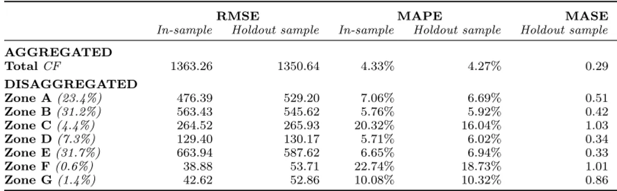
The best performing forecasting model for aggregated data, CF, is used to produce forecasts at zone level. The results are shown in table 5. The percentages in the first column represent the
Table 4. Top-down approach: analysis absolute scaled error (ASE) for the out-of-sample aggre-gated forecast.
MASE σ ASE Minimum ASE Maximum ASE
Current 0.33 0.27 0.00 1.46 Na¨ıve I 0.89 0.61 0.00 3.19 MA(5) 0.58 0.44 0.01 2.20 wMA(5) 0.37 0.29 0.00 1.32 ES(N-N) α = 0, 106 0.61 0.43 0.00 2.24 ES(A-N) α = 0, 106 β = 0, 000 0.61 0.43 0.00 2.23 ES(N-M) α = 0, 174 γ = 0, 114 0.30 0.25 0.00 1.27 AR(4) 0.36 0.29 0.00 1.30 ARMA(4; 1) 0.36 0.28 0.00 1.28 ARIMA(4; 1; 1) 0.37 0.28 0.00 1.33 SARIMA (3; 0; 1)(0; 1; 1)5 0.31 0.26 0.01 1.21 ARIMAX(2 ; 1; 1) 0.31 0.27 0.00 1.41 CF ES(N-M)
& SARIMA & ARIMAX
0.29 0.25 0.00 1.25
average daily fraction of the total number of each zone’s order lines. The scaled error MASE, which is independent of the data scale, is used to compare the accuracy of forecasts at zone level.
Forecasts for the three large zones (i.e., zones A, B, and E), as well as zone D, are accurate using the top-down approach. Forecasting errors of those four order picking zones are on average a factor of 0.33 to 0.51 smaller than the in-sample forecasting errors from the na¨ıve method. A slightly bigger forecasting error is produced in zone G. In the remaining two zones, C and F, the top-down approach does not forecast the daily number of order lines as successfully as the na¨ıve method’s in-sample forecasting values.
Table 5. Top-down approach: forecasting accuracy aggregated and disaggregated forecast.
RMSE MAPE MASE
In-sample Holdout sample In-sample Holdout sample Holdout sample AGGREGATED Total CF 1363.26 1350.64 4.33% 4.27% 0.29 DISAGGREGATED Zone A (23.4%) 476.39 529.20 7.06% 6.69% 0.51 Zone B (31.2%) 563.43 545.62 5.76% 5.92% 0.42 Zone C (4.4%) 264.52 265.93 20.32% 16.04% 1.03 Zone D (7.3%) 129.40 130.17 5.71% 6.02% 0.34 Zone E (31.7%) 663.94 587.62 6.65% 6.94% 0.33 Zone F (0.6%) 38.88 53.71 22.74% 18.73% 1.01 Zone G (1.4%) 42.62 52.86 10.08% 10.32% 0.86
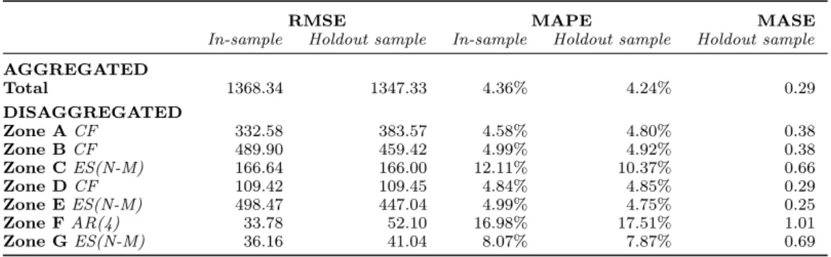
4.2 Bottom-up Forecasting Approach
In the bottom-up forecasting approach, the daily number of order lines is forecast for each individual zone. All time series models presented in table 1 are applied to each order picking zone. Forecasting accuracy measures of the best performing model are summarized in table 6. These disaggregated forecasts are accumulated to produce the aggregated demand. Again, MASE is used to compare forecasts of all order picking zones.
Comparison of disaggregated demand using the bottom-up forecasting process results in similar conclusions as in the previous section. Order lines of the main four order picking zones, in particular
Table 6. Bottom-up approach: forecasting accuracy aggregated and disaggregated forecast.
RMSE MAPE MASE
In-sample Holdout sample In-sample Holdout sample Holdout sample AGGREGATED Total 1368.34 1347.33 4.36% 4.24% 0.29 DISAGGREGATED Zone A CF 332.58 383.57 4.58% 4.80% 0.38 Zone B CF 489.90 459.42 4.99% 4.92% 0.38 Zone C ES(N-M) 166.64 166.00 12.11% 10.37% 0.66 Zone D CF 109.42 109.45 4.84% 4.85% 0.29 Zone E ES(N-M) 498.47 447.04 4.99% 4.75% 0.25 Zone F AR(4) 33.78 52.10 16.98% 17.51% 1.01 Zone G ES(N-M) 36.16 41.04 8.07% 7.87% 0.69
zones A, B, D, and E, can be forecast highly accurately. Forecasting errors are on average a factor of 0.25 to 0.38 smaller than the in-sample forecasting errors from the na¨ıve method. The AR(4) model outperforms all other forecasting models only in zone F. However, the forecasting errors resulting from the autoregressive model are rather large. The ES(N-M) forecasting model results in the most accurate forecasts in zones C, E, and G. Other order picking zones are most accurately forecast using the composite forecasting technique.
4.3 Comparing Top-down and Bottom-up Forecasting
A paired-samples t-test is used to compare forecasting errors of the top-down and bottom-up forecasting process. Differences of the scale independent forecasting accuracy measures, including MAPE and MASE, are tested for the out-of-sample forecasting values. In the first t-test, the mean absolute forecasting error of the top-down forecasting process is compared to MAPE of the bottom-up approach. Secondly, MASE of both forecasting approaches are compared. Differences of performances between the top-down and bottom-up approaches, both relative difference and absolute difference, as well as results of the two-sided paired-samples t-tests are summarized in table 7. First, the disaggregated test results are presented, followed by the aggregated performance differences among the top-down and bottom-up forecasting approaches.
Table 7. 2-tailed significance levels for the paired-samples t tests on mean difference for the top-down and bottom-up forecasting approach. MAPE MASE relative ∆M AP E absolute ∆M AP E
st. dev. t df sign. relative ∆M ASE absolute ∆M ASE st. dev. t df sign. AGGREGATED Total -0.55% -0.02 pp 0.54 pp 0.67 238 0.504 -0.39% 0.00 0.04 0.48 238 0.631 DISAGGREGATED Zone A -28.31% -1.89 pp 4.95 pp 5.92 238 0.000 -24.28% -0.12 0.37 5.12 238 0.000 Zone B -16.84% -1.00 pp 3.70 pp 4.17 238 0.000 -8.90% -0.04 0.27 2.14 238 0.033 Zone C -35.34% -5.67 pp 13.01 pp 6.74 238 0.000 -36.02% -0.37 0.92 6.21 238 0.000 Zone D -19.34% -1.16 pp 3.89 pp 4.62 238 0.000 -14.99% -0.05 0.22 3.49 238 0.001 Zone E -31.53% -2.19 pp 4.75 pp 7.12 238 0.000 -25.84% -0.09 0.23 5.79 238 0.000 Zone F -6.49% -1.21 pp 12.64 pp 1.49 238 0.139 -0.44% 0.00 0.64 0.11 238 0.914 Zone G -23.76% -2.45 pp 7.31 pp 5.19 238 0.000 -19.95% -0.17 0.61 4.36 238 0.000 ∆M AP E = difference between bottom-up MAPE and top-down MAPE
∆M ASE= difference between bottom-up MASE and top-down MASE
df = degrees of freedom pp = percentage point
sign. = significance level of the two-sided paired-samples t-test st. dev. = standard deviation
Significance levels of both accuracy measures are consistent in determining the best disaggregated forecasting approach. For all order picking zones, except for zone F, the bottom-up approach results in statistically significant lower forecasting errors, while for zone F the null hypothesis of equal forecasting errors cannot be rejected. This result can be explained by the fact that an equal daily distribution of total order lines across zones, as assumed in the top-down approach, is rather unlikely to occur. In the bottom-up forecasting process, daily number of order lines is forecast for each single order picking zone, resulting in a variable fraction of each zone’s demand in total demand. Zone F is one of the smaller order picking zones in the warehouse in which the seasonal pattern is less clear compared to other order picking zones. The strong fluctuating demand as well as the absence of a weekly recurring cycle results in large forecasting errors in both forecasting approaches.
Forecasting errors of aggregated demand prediction using a top-down approach are compared to the bottom-up approach in an equivalent way. Neither percentage errors nor the scaled errors are statistically significantly different using the CF forecasting model for aggregated demand or accumulating the disaggregated forecasts. As a large amount of the order line variation of each single zone can be explained by the time series forecasting methods in the main order picking zones, the derived aggregated forecasting in the bottom-up approach is a reliable forecast of the real total number of order lines. As the time series forecasting models are able to reliably forecast the total number of order lines in the top-down approach, as well, the null hypothesis of equal forecasting errors cannot be rejected.
From the results in table 7, it can be concluded that the bottom-up approach outperforms the top-down approach in forecasting disaggregated demand, except for forecasting order lines in zone F. Average forecasting errors for predicting neither the total number of order lines nor the order lines in zone F are statistically significantly different.
5. Conclusions
Workload forecasting is an essential activity in the labour-intensive environment of warehouses. However, workforce related studies in warehouses are limited. The objective of this study was to find well-performing time series models in order to accurately forecast order pickers’ workload using real-life order line data. Accurate planning is required in order to provide a high service level, as well as to avoid unnecessary high labour costs. This clearly shows the added value of our work in practice.
The results of the study show that the total number of order lines in the case study can be forecast in a highly accurate way. Several presented forecasting models are able to outperform the benchmark, i.e., the non-statistical forecasts done by supervisors. The combined forecasting method results in most accurate predictions for daily total number of order lines, followed by the exponential smoothing model with multiplicative weekly seasonality, the full SARIMA model, and the ARIMAX forecasting model.
As warehouses are often divided into different order picking zones to achieve a more efficient order picking process, planning of order pickers is done at zone level. For those planning purposes, forecasting order lines should be disaggregated. More accurate forecasts are produced by using a bottom-up forecasting approach, to the detriment of a top-down forecasting approach. The CF and the ES(N-M) forecasting models have proven to be especially useful in predicting the number of order lines at the zone level.
As a result of our study, the daily forecasts produced by the forecasting models are currently used by the warehouse supervisors to determine the daily required number of order pickers and to allocate order pickers across zones. Based on the average productivity of order pickers in the warehouse, the mean absolute forecasting error in number of full-time equivalents (FTEs) could have been reduced from 10 to 7 in 2013 and from 8 to 7 in 2014 by using the composite forecasting
method to predict the total number of order lines. This means that, on average, the daily number of either overestimated or underestimated number of order pickers could have been reduced by 1–3 FTEs. Moreover, the planning of order pickers will be less depending on the availability of experienced supervisors, as the forecasting methods are able to accurately predict both aggregated and disaggregated demand without manual intervention.
The methods and results of our study contribute to both practitioners and academic research. The evaluation of an extensive range of time series forecasting models helps warehouse managers to select methods able to reliably forecast the order lines of a zone picking warehouse. The forecasting methods of our study can be easily implemented, and the implementation immediately helps ware-house managers to plan order pickers. Furthermore, the results of this study are a starting point for further workforce related research in warehouses. This paper is limited to workload forecasting in an order picking process and could be enlarged to other warehouse operations (e.g., inbound activities) or other warehouses (e.g., progressive zoning warehouse) in order to further generalize the conclusions of our study.
Future research in the problem area of workforce planning in warehouses could include analysis of other personnel capacity planning steps (i.e., determining staffing requirements, shift scheduling, and shift assignment). The forecasting methods presented in this paper can serve as input for the planning of a flexible workforce. The effects of cross-training and transferring order pickers on warehouse performances could be analysed, as the flexible workforce scheduling problem in a zone picking warehouse allows workers to transfer to other order picking zones in order to pick all orders.
References
Athanasopoulos, George, Rob J. Hyndman, Haiyan Song, and Doris C. Wu. 2011. “The tourism forecasting competition.” International Journal of Forecasting 27 (3): 822–844.
Chase Jr, Charles W. 2013. Demand-driven forecasting: a structured approach to forecasting. John Wiley & Sons.
Cools, Mario, Elke Moons, and Geert Wets. 2009. “Investigating the Variability in Daily Traffic Counts Through Use of ARIMAX and SARIMAX Models: Assessing the Effect of Holidays on Two Site Loca-tions.” Transportation Research Record: Journal of the Transportation Research Board 2136 (-1): 57–66. Davarzani, Hoda, and Andreas Norrman. 2015. “Toward a relevant agenda for warehousing research:
liter-ature review and practitioners´ input.” Logistics Research 8 (1): 1–18.
De Gooijer, Jan G., and Rob J. Hyndman. 2006. “25 years of time series forecasting.” International Journal of Forecasting 22 (3): 443–473.
De Koster, Ren´e B. M., Tho Le-Duc, and Kees Jan Roodbergen. 2007. “Design and control of warehouse order picking: A literature review.” European Journal of Operational Research 182 (2): 481–501.
De Koster, Ren´e B. M., Tho Le-Duc, and Nima Zaerpour. 2012. “Determining the number of zones in a pick-and-sort order picking system.” International Journal of Production Research 50 (3): 757–771. Defraeye, Mieke, and Inneke Van Nieuwenhuyse. 2016. “Staffing and scheduling under nonstationary demand
for service: A literature review.” Omega 58: 4–25.
Gardner Jr., Everette S. 2006. “Exponential smoothing: The state of the art - Part II.” International Journal of Forecasting 22 (4): 637–666.
Goh, Carey, and Rob Law. 2002. “Modeling and forecasting tourism demand for arrivals with stochastic nonstationary seasonality and intervention.” Tourism Management 23 (5): 499–510.
Gu, Jinxiang, Marc Goetschalckx, and Leon F. McGinnis. 2007. “Research on warehouse operation: A comprehensive review.” European Journal of Operational Research 177 (1): 1–21.
Gu, Jinxiang, Marc Goetschalckx, and Leon F. McGinnis. 2010. “Research on warehouse design and perfor-mance evaluation: A comprehensive review.” European Journal of Operational Research 203 (3): 539–549. House-Peters, Lily A., and Heejun Chang. 2011. “Urban water demand modeling: Review of concepts,
methods, and organizing principles.” Water Resources Research 47 (5): W05401.
Hwang, H., and D. G. Kim. 2005. “Order-batching heuristics based on cluster analysis in a low-level picker-to-part warehousing system.” International Journal of Production Research 43 (17): 3657–3670.
Hyndman, Rob J., and Anne B. Koehler. 2006. “Another look at measures of forecast accuracy.” Interna-tional Journal of Forecasting 22 (4): 679–688.
Jacobs, F. Robert, Richard B. Chase, and Richard Chase. 2010. Operations and supply chain management. McGraw-Hill/Irwin.
Jane, Chin-Chia. 2000. “Storage location assignment in a distribution center.” International Journal of Physical Distribution & Logistics Management 30 (1): 55–71.
Jane, Chin-Chia, and Yih-Wenn Laih. 2005. “A clustering algorithm for item assignment in a synchronized zone order picking system.” European Journal of Operational Research 166 (2): 489–496.
Koo, Pyung-Hoi. 2008. “The use of bucket brigades in zone order picking systems.” OR Spectrum 31 (4): 759–774.
Le-Duc, Tho, and Ren´e B. M. De Koster. 2005. Determining Number of Zones in a Pick-and-pack Order-picking System. Technical Report ERS-2005-029-LIS. ERIM Report Series Research in Management. Rouwenhorst, B., B. Reuter, V. Stockrahm, G. J. van Houtum, R. J. Mantel, and W. H. M. Zijm. 2000.
“Warehouse design and control: Framework and literature review.” European Journal of Operational Research 122 (3): 515–533.
Ruben, Robert A., and F. Robert Jacobs. 1999. “Batch Construction Heuristics and Storage Assignment Strategies for Walk/Ride and Pick Systems.” Management Science 45 (4): 575–596.
Sanders, Nada R., and Larry P. Ritzman. 2004. “Using Warehouse Workforce Flexibility to Offset Forecast Errors.” Journal of Business Logistics 25 (2): 251–269.
Schwarzkopf, Albert B., Richard J. Tersine, and John S. Morris. 1988. “Top-down versus bottom-up fore-casting strategies.” International Journal of Production Research 26 (11): 1833.
Song, Haiyan, and Gang Li. 2008. “Tourism demand modelling and forecasting– A review of recent research.” Tourism Management 29 (2): 203–220.
Suganthi, L., and Anand A. Samuel. 2012. “Energy models for demand forecasting– A review.” Renewable and Sustainable Energy Reviews 16 (2): 1223–1240.
Van Gils, Teun, Katrien Ramaekers, Kris Braekers, and An Caris. 2015. “Improving Operational Work-force Scheduling in a Warehouse Using Time Series Forecasting.” Abstract from European conference for Operational Research 2015, Glasgow, United Kingdom.
Zotteri, Giulio, Matteo Kalchschmidt, and Federico Caniato. 2005. “The impact of aggregation level on forecasting performance.” International Journal of Production Economics 93-94: 479–491.