Using a Visual Structured Criterion for the Analysis of Alternating-Treatment Designs Marc J. Lanovaz
Université de Montréal and Centre de recherche du CHU Sainte-Justine Patrick Cardinal
École de Technologie Supérieure Mary Francis
Université de Montréal
Author Note
This research project was supported in part by a salary award from the Fonds de Recherche du Québec – Santé (#30827) to the first author. We thank Dr. John M. Ferron for providing a copy of his SAS permutation analysis procedure, which we used to validate the script for the current project.
Correspondence concerning this article should be addressed to Marc J. Lanovaz, École de Psychoéducation, Université de Montréal, C.P. 6128, succursale Centre-Ville, Montreal, QC, Canada, H3C 3J7.
Email: [email protected]
The final, definitive version of this paper has been published in Behavior Modification, 43/1, January 2019 published by SAGE Publishing, All rights reserved.
Abstract
Although visual inspection remains common in the analysis of single-case designs, the lack of agreement between raters is an issue that may seriously compromise its validity. Thus, the purpose of our study was to develop and examine the properties of a simple structured criterion to supplement the visual analysis of alternating-treatment designs. To this end, we generated simulated datasets with varying number of points, number of conditions, effect sizes and autocorrelations, and then measured Type I error rates and power produced by the visual structured criterion (VSC) and permutation analyses. We also validated the results for Type I error rates using nonsimulated data. Overall, our results indicate that using the VSC as a supplement for the analysis of systematically alternating-treatment designs with at least five points per condition generally provides adequate control over Type I error rates and sufficient power to detect most behavior changes.
Keywords: alternating-treatment design, Monte Carlo simulation, multielement design, power, Type I error, visual analysis
Using a Visual Structured Criterion for the Analysis of Alternating-Treatment Designs Alternating-treatment designs (ATDs) have been widely adopted to assess and to compare the effects of interventions in applied settings (Manolov & Onghena, 2017).
Oftentimes, both practitioners and researchers rely on the visual inspection of ATDs to determine whether the implementation of an intervention is responsible for changes observed in a target behavior (Kratochwill et al., 2010; Lane & Gast, 2014; Ninci, Vannest, Willson, & Zhang, 2015). However, researchers have shown that the lack of agreement between raters remains an issue that may seriously compromise the validity of the visual analysis of these designs (Diller, Barry, & Gelino, 2016; Hagopian et al., 1997). This lack of agreement increases the probability of reaching incorrect conclusions regarding functional relations.
Practitioners and researchers can make two type of errors when analyzing the results of single-case experiments. Type I errors, also referred to as false positives, occur when a
practitioner or researcher concludes that a functional relation exists when one does not. In contrast, Type II errors, also referred to as false negatives, occur when a practitioner or
researcher concludes that a functional relation does not exist when one does. Type II error rates are typically expressed in terms of power, which represents the probability of detecting a functional relation when one actually exists. Generally, researchers aim to design experiments that produce Type I error rates of less than .05 and power of more than .80 (Cohen, 1992).
One potential solution to minimize issues related to interrater agreement is to use structured aids that support researchers and practitioners in their visual analyses. For example, Hagopian et al. (1997) developed structured criteria to support decision-making for functional analyses conducted using ATDs with multiple conditions. These criteria were subsequently adapted and applied for the analysis of pairwise designs (i.e., ATDs with only two conditions;
Hagopian, Rooker, Jessel, & DeLeon, 2013; Roane, Fisher, Kelley, Mevers, & Bouxsein, 2013). The structured analyses involved tracing two confidence lines (one standard deviation above and below the mean of the control condition), counting the number of data points above and below the confidence lines, and then applying a series of rules to identify the function of the behavior. Albeit promising for the interpretation of functional analyses, these methods have numerous steps, which can make them complex, and have not been the topic of studies examining their Type I error rates and power.
In another example, Bartlett, Rapp, and Henrickson (2011) developed visual criteria to analyze Type I error rates obtained in brief ATDs using operational definitions of stability and trend. In their study, the raters considered data paths differentiated when there was no or minimal overlap between paths, and “(a) two or more data paths were stable with at least 5% separation, (b) two or more data paths were trending in opposite directions, or (c) one data path was stable and the other data path was trending away from it” (p. 537). The criteria adequately controlled for Type I error rates for pairwise comparisons with three to five points per condition, but the study did not examine power, nor the impact of autocorrelation on the results of their analyses.
Autocorrelation is a common phenomenon observed in single-case designs wherein data points are partly correlated with the data points preceding them (Shadish & Sullivan, 2011). In other words, it represents the correlation between measures of the same behavior across sessions. From a behavioral standpoint, autocorrelation may be the result of both controlled and
uncontrolled variables such as physiological states and motivating operations. According to Shadish and Sullivan (2011), the mean autocorrelation in published single-case research in 2008 was .20 and the values from individual studies had an extensive range (from -.93 to .79). For ATDs only, mean corrected autocorrelation did not differ significantly from zero, but we can
assume that variability across studies remained high as reported in the overall range. Consequently, analyses must consider different values of autocorrelation as they have a significant impact on Type I error rates and power in ATDs (Levin, Ferron, & Kratochwill, 2012).
In a study examining the impact of autocorrelation on visual structured criteria in single-case designs, Fisher, Kelley, and Lomas (2003) developed the dual-criteria and conservative dual-criteria methods, which involve tracing a continuation of the mean and trend lines from baseline to analyze AB, reversal, and multiple baseline designs. Their study showed that the conservative method produced acceptable Type I error rates and power, and that increasing autocorrelation led to small increases in Type I error rate. That said, their method is not applicable to ATDs because the baseline sessions are not conducted consecutively. Thus, the purpose of our study was to develop a simple structured criterion for the visual analysis of ATDs, and then to examine its Type I error rate and power using simulated and nonsimulated data with various number of points, number of conditions, effect sizes, and autocorrelations.
Development of the Structured Visual Criterion
Probably the simplest and most straightforward procedure to compare two conditions within an ATD is to examine whether the paths overlap, which can be done by counting the number of sessions the path and points for one condition are above or below the other. This approach would be similar to the nonoverlap methods used to calculate effect sizes in ATDs such as the percentage of nonoverlapping data and the nonoverlap of all pairs (Parker & Vannest, 2009; Wolery, Gast, & Hammond, 2010). In these cases, the overlap is compared on a point-by-point basis (e.g., first point-by-point with first point-by-point, second point-by-point with second point-by-point) in contrast with the methodology that we propose, which compares the relative position of paths and points (see
below). The nonoverlap methods do not consider trend and may produce values of 100%
nonoverlap even when the data paths cross (Manolov & Onghena, 2017). Therefore, we adopted an approach that considered both paths and points. One concern with considering overlap is that the probability of paths crossing due to extraneous variables increases with the number of points. In other words, researchers and practitioners may observe data paths crossing even when an independent variable has a true effect on behavior, which can lead to false negatives. To address this issue while taking advantage of the simplicity of comparing the position of both paths, we developed the visual structured criterion (VSC), a visual analysis method relying on the relative position of both paths across sessions.
Specifically, the VSC involves two simple steps. First, the practitioner or researcher counts the number of times that the data path and points for one condition fall above (or below for interventions designed to reduce behavior) the data path and points of a second condition at each session of either condition. In other words, a comparison is conducted whenever the following conditions are met: (a) a session contains a data point for one of the two conditions being compared and (b) a path is present for the other condition being compared at this same session’s location on the graph. For a systematically alternating design, the initial data point of the first condition and the last data point of the second condition are ignored as there is no path to compare each point with at these locations. As such, the number of comparisons is the total number of points of both conditions minus two (i.e., the first and last points where there are no paths to compare). When the ATD includes more than two conditions, the data points and paths for the additional conditions (i.e., not being compared) are also ignored. This logic is consistent with the actual and linearly interpolated values (ALIV) method recently developed and proposed
by Manolov and Onghena (2017), which excludes points when path overlap is impossible (e.g., first and last sessions) and relies on linearly interpolated values during their analyses.
Second, the number of times that the data path and points for one condition fall above (or below) those of the second condition is compared to the cut-off values provided in Table 1. We provide the cut-off values for both the number of points per condition (only if equal) and for the number of comparisons. We also included a percentage measure for the cut-off, which should facilitate comparisons with other nonoverlap methods. Note that the cut-off percentage initially decreases in a staggered fashion (with occasional increases), which is caused by the discrete nature of the distribution. If the actual value is equal to or larger than the cut-off value, we can consider that the analysis has detected an effect of the independent variable.
We empirically derived the cut-off values reported in Table 1 to maximize power while maintaining Type I error rates near or below .05 given no autocorrelation. That is, we first generated 100,000 datasets with no autocorrelation containing 5 to 12 points per condition (see Monte Carlo Validation for detailed procedures). The number of potential comparisons varied according to the number of points (see Table 1). Then, we instructed the spreadsheet to compute Type I error rates and power when the cut-off value was set at its maximum possible value (i.e., the number of comparisons). Finally, we gradually decreased the cut-off value until we found the lowest cut-off value that would still maintain Type I error rates near or below .05. This procedure allowed us to maximize power while still providing adequate control over Type I error rates.
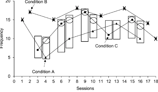
To illustrate the use of the VSC, assume that Figure 1 represents the frequency of a behavior occurring during condition A (baseline), condition B (intervention 1), and condition C (intervention 2) across 18 sessions in total (six per condition). Further assume that the purpose of both interventions is to increase the frequency of the behavior and that we aim to compare A with
C. The first step would be to count the number of times that the data path and points for
condition C fall above the data path and points for condition A at each session of either condition (i.e., sessions 3, 4, 6, 7, 9, 10, 12, 13, 15, and 16); in this example, we have ten comparisons for A and C (see rectangles in Figure 1). We ignore the first data point of A (i.e., 1) and the last data point of C (i.e., 18) as only there is no path from the other condition to compare each point with, and we exclude all data points during which we implemented condition B (i.e., sessions 2, 5, 8, 11, 14, and 17). In our example, the data path and points for condition C fall above the data path and points for condition A 7 times (see circles within rectangles in Figure 1). The second step is to compare this value (i.e., 7) to the value for ten comparisons in Table 1 (i.e., 9). Given that 7 is not equal to or higher than 9, we can conclude that the difference observed could have occurred by random fluctuation. Note that the exact same procedure could be repeated to compare A with B and B with C. For the purpose of the current study, the second author wrote a Python script (Cardinal & Lanovaz, 2017), which conducted the analyses automatically.
Experiment 1 – Monte Carlo Validation
One important step when validating a novel approach to analysis is to examine Type I error rates and power from a very large number of datasets with specific parameters and to compare these results to those of a well-established method. To this end, we conducted a Monte Carlo validation to set our cut-off values and to examine the effects of number of points, number of conditions, effect sizes and autocorrelations. Then, we compared our results with those
produced by permutation analyses using the same datasets. Data Generation
We used R (R Core Team, 2017) to generate datasets containing 6 to 20 points.
normal distribution with a mean of 0 and a standard deviation of 1 for different values of first-order autocorrelation. To prevent negative values during analyses, the program then added a constant of 10 to all data points. For each set of parameters described in our analyses, we instructed R to generate 100,000 datasets.
For our power analyses, we also added an effect size parameter to every second point in each dataset, which simulated the introduction of an independent variable within a pairwise design in which the A and B conditions were alternated systematically (i.e., ABABAB…AB). The effect size parameter was a measure of mean behavior change in standard deviations (equivalent to Cohen’s d). It should be noted that the traditional rules of thumb developed for Cohen’s d (see Cohen, 1992) do not apply to single-case designs. Whereas a d value of 1 may be considered a large effect size in a randomized controlled trial, the same value in single-case research may be considered very small (Levin, Lall, & Kratochwill, 2011). For example, Marquis et al. (2000) found that the lowest reliable effect size measure for positive behavior support interventions was 1.5. More recently, Rogers and Graham (2008) reported that effect sizes were typically 3 or higher when applying this measure to single-case research examining writing treatments. For the current study, we thus set the values of effect sizes at 1, 2, and 3. Analyses
Effects of number of points per condition. For our initial analyses, we examined Type I error rates and power produced by the VSC for systematically alternating pairwise designs (i.e., i.e., ABABAB…AB) for different number of points per condition, which allowed us to set our cut-offs for Table 1. For these initial analyses, the number of points per condition varied from 3 to 12 points and the autocorrelation was held constant at 0. To calculate Type I error rates, we divided the number of datasets for which the VSC detected an effect by the total number of data
sets (i.e., 100,000). Next, we examined the power of the VSC for effect sizes of 1, 2 and 3 with no autocorrelation for the same number of points per condition. We calculated power using the same formula as for the Type I error rates; the only difference was that d was no longer 0.
Effects of number of conditions. Next, we replicated the previous analyses for ATDs with more than two conditions alternated systematically (i.e., ABCABC…ABC,
ABCDABCD…ABCD, and ABCDEABCDE…ABCDE). The number of points per condition was held constant at six and the autocorrelation remained 0. Given that the order of the
conditions may impact Type I error rates and power, we averaged the values obtained by comparing each treatment condition (i.e., B, C, D, and E) with the baseline condition A.
Comparison of the VSC with permutation analyses. In our final analyses for the first
experiment, we compared Type I error rates and power (for an effect size of 2) for pairwise designs produced by the VSC with those yielded by permutation analyses for different values of autocorrelation. We selected permutation analysis as a comparison because (a) it is
nonparametric (i.e., no assumption regarding normality of distribution), (b) it provides adequate control over Type I errors and sufficient power, and (c) it has been recommended for use with ATDs (see Levin et al., 2012). For our permutation analysis, we calculated the Type I error rates and power by dividing the number of datasets where p < .05 by the total number of datasets (i.e., 100,000). Although our design involved a systematic alternation of AB conditions, we used a complete randomization scheme in order to replicate the permutation procedures proposed by Levin et al. (2012).
To compute the p values for permutation analyses, the second author wrote a second Pythonscript (Cardinal & Lanovaz, 2017), which completed the following steps for each dataset. First, the script instructed the program to compute the difference between the mean of all points
in condition B and the mean of all points in condition A for the original dataset. Second, the program divided the original data points into two equal-sized groups, regardless of their initial condition assignment. We designed the script so that it would generate all the possible sets of two equal-sized groups, which resulted in 924 combinations for six points per condition and 184,756 combinations for ten points per condition. Then, the script repeated the first step with all these combinations. Fourth, the script ranked the original dataset with all the combinations by decreasing order of the difference between the means of both conditions. Finally, the analysis produced a p value by dividing the rank of the original dataset by the total number of
combinations.
Results and Discussion
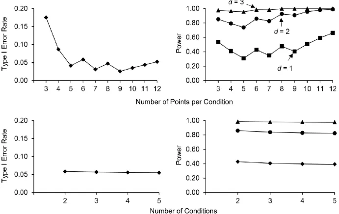
Figure 2 presents Type I error rates (left panels) and power (right panels) for different sets of parameters. We did not include error bars for the 95% confidence interval on the first two figures as they would have been too narrow to draw; the plus or minus values of the 95%
confidence interval ranged from .001 to .003, which is very small. The upper panels of Figure 2 show the results of our initial analyses examining the effects of varying the number of points in a pairwise design. Type I error rates for the VSC method remained acceptable as soon as the ATD contained at least five points per condition. Power was also generally adequate for effect sizes of 2 and 3, which are typically observed in single-case designs. The upper middle panels present the effects of increasing the number of conditions when each condition had six points. Both Type I error rates and power decreased marginally when the number of conditions increased, but remained within acceptable boundaries (i.e., Type I error rates near .05 and power higher than .80).
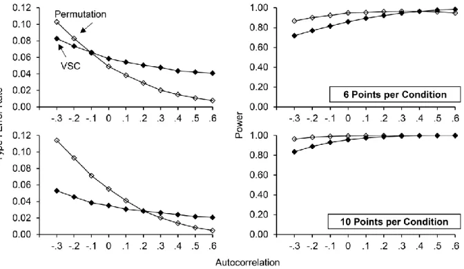
Figure 3 compares the error rates and power of the VSC with the results of permutation analyses. The VSC provided better control over Type I errors for negative autocorrelation (for both six and ten points per condition) and for low values of positive autocorrelation (for ten points per condition) whereas permutation analyses were more stringent for high positive values of autocorrelation. In contrast, power was typically higher for permutation analyses, except for large positive autocorrelations for which we observed marginally higher power for the VSC at six points per condition. Altogether, the results of the first experiment suggest that the VSC adequately controls for Type I error rate and has sufficient power for detecting typical effect sizes (i.e., 2 or more) observed in single-case designs.
Experiment 2 – Validation Using Nonsimulated Data
One of the drawbacks of using Monte Carlo simulations is that the datasets may not perfectly mimic patterns of behavior observed in the natural environment. As such, it is important to examine whether the properties of the methodology would remain the same for nonsimulated data. To this end, we examined to what extent the VSC would detect changes in extended baselines. Given that no independent is introduced during baseline, any detection of an effect would be considered as a Type I error rate.
Procedures
To examine Type I error rates, we used the same extended baseline datasets that we had previously extracted for a study examining false positives in AB, reversal, and multiple baseline designs (see Lanovaz, Huxley, & Dufour, 2017 for detailed procedures). We extracted these baseline data from 295 graphs included in 73 articles published in the 2013 and 2014 volumes of the Journal of Applied Behavior Analysis, Behavior Modification, Behavioral Interventions and Journal of Positive Behavior Interventions. Each graph included an initial baseline phase
containing 6 to 20 data points, which we used for our analyses. We used extended baselines rather than ATDs for this analysis because our purpose was to measure Type I error rates. To identify false positives, we must use datasets in which no independent variable is introduced (i.e., we must observe a change in the absence of an independent variable). It was thus not possible to use ATDs for this purpose as any observed change could have been attributed to the independent variable and would have prevented the calculation of Type I error rates.
For analysis, we divided each extended baseline into datasets containing all possible ordered combinations of 6, 8, 10, 12, and 14 data points. For example, assume that a baseline phase contained 12 data points, which we numbered in order from 1 to 12. Such a baseline phase would produce seven 6-point datasets (points 1 to 6, 2 to 7, 3 to 8, 4 to 9, 5 to 10, 6 to 11, 7 to 12), five 8-point datasets (points 1 to 8, 2 to 9, 3 to 10, 4 to 11, 5 to 12), three 10-point datasets (1 to 10, 2 to 11, 3 to 12), one 12-point dataset (points 1 to 12) and no 14-point datasets. In total, our data preparation yielded 4,854 datasets for analysis. Then, we took each dataset and assigned the odd-numbered points to condition A and the even-numbered points to condition B. Finally, we applied the VSC to each dataset using our Python script and calculated the Type I error rate for 3, 4, 5, 6 and 7 points per condition by dividing the number of changes detected by the VSC by the total number of datasets for a given number of points per condition. Given that our data preparation yielded more datasets containing 3 points per condition than 7 points per condition, we also calculated the 95% confidence interval for each proportion.
Initially, we had also extracted datasets containing 8, 9 and 10 points per condition (i.e., 16, 18, and 20 points in total). Although the Type I error rates were consistent with the results of the first experiment, the ranges of the 95% confidence intervals were too large to draw any
useful conclusions (as we had too few datasets with 16 to 20 points). Therefore, we do not report these analyses in our results.
Results and Discussion
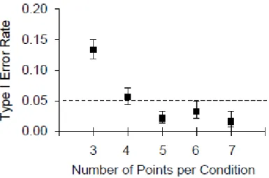
Figure 4 shows the Type I error rate for different number of points per condition produced by the VSC on nonsimulated datasets. As soon as the design contained at least five points per condition, Type I error rates remained below the threshold value of .05. When compared to Type I error rates obtained with nonsimulated data (see upper left panel of Figure 2), the error rates for the simulated data were lower. One potential explanation for this result is that our nonsimulated datasets may have been autocorrelated, which was not the case for the simulated data that we used to set the cut-offs. Positive autocorrelations tend to reduce Type I error rates in ATDs.
General Discussion
Overall, our results indicate that using the VSC as a supplement for the analysis of ATDs with at least five points per condition generally provides adequate control over Type I error rates and sufficient power for behavior changes typically observed in single-case designs.
Interestingly, the VSC produced lower Type I error rates than permutations analyses for negative (for both six and ten points per condition) and lower positive (for ten points per condition) autocorrelations. Contrarily, permutation analyses had higher power than the VSC under similar parameters. Moreover, increasing levels of autocorrelation decreased Type I error rates when using the VSC, which is opposite to the pattern observed by Fisher et al. (2003). This result is most likely due to the distribution of the error across designs produced by the autocorrelation. In reversal and multiple baseline designs, the autocorrelated error is mostly distributed within conditions whereas it is mostly distributed across conditions within ATDs. As such, the
variability (error term) is more evenly distributed across conditions in ATDs, which makes the detection of effects more likely. These patterns are consistent with those obtained by Levin et al. (2012) using nonparametric permutation analyses. Our results are also consistent with the What Works Clearing House criteria for well-designed experiments, which recommends conducting at least five replications of systematically alternating sequence when using ATDs (Kratochwill et al., 2010). However, ATDs using randomized block designs may require more than five points per condition to achieve five replications, unless the comparisons are performed in blocks of two (e.g., AB-BA-BA-AB) or a maximum of two consecutive measurement times for each condition is allowed.
Compared to other methods for the analysis of ATDs (e.g., Hagopian et al., 1997; Roane et al., 2013), the VSC involves fewer steps, which reduces complexity and the probability of making errors during analysis. Furthermore, the VSC is the only method for ATDs for which both Type I error rates and power have been documented. Our results indicate that researchers and practitioners may adopt the VSC to supplement their analyses whenever they compare two or more conditions within an ATD. For example, the VSC may be used to evaluate the effects of an intervention in relation to baseline, to contrast the effects of two interventions, or to compare the control condition with the test conditions in a functional analysis. Applying the VSC to any of the previous situations will increase the confidence that the observed differences are the result of the intervention, or variable introduced, and not the product of naturally occurring patterns of behavior. To further increase the confidence in the results, the practitioner or researcher could use a randomized block design or a randomization scheme with the restriction of a maximum of two consecutive measurements per condition (see Onghena & Edgington, 1994) instead of using systematic alternations as we have done in the current study. That being said, it should be noted
that regardless of the type of randomization scheme adopted, the VSC alone cannot determine whether an observed change is socially significant. If the VSC detects a behavior change, practitioners and researchers should continue relying on visual analysis or use other effect size measures (see Parker, Vannest, & Davis, 2011 for review) to determine whether this observed change is socially significant for the person.
Our results are limited insofar as we only examined the effects of the VSC for ATDs with systematic alternations. We also included an equal number of data points in each condition. According to Manolov and Onghena (2017), 36% of published ATDs have an equal number of measurements for each condition. Given that the distribution of error across conditions would differ, researchers should consider replicating our study with random assignment of conditions (rather than alternating) and with conditions that contain unequal numbers of sessions. A second limitation is that we did not examine whether researchers and practitioners could readily learn how to apply the VSC. Although the VSC is simpler than other methods as it involves only two steps and does not involve the determination of trend or confidence lines, researchers should still conduct studies examining its applicability in the future. Third, we did not conduct a power analysis with nonsimulated data. Unfortunately, it is not possible to conduct power analyses without being tautological as the only way to determine whether the introduction of an
independent variable influenced a behavior using nonsimulated data is to apply rules of analyses. Nonetheless, we did compare power with another established method (i.e., permutation analyses) to address this issue in the first experiment.
Fourth, we limited our comparison of the VSC to permutation analyses. In the future, researchers should consider comparing the VSC with established effect sizes measures (e.g., percentage of points exceeding the median, percentage of nonoverlapping points). Similarly, our
study is limited insofar as we did not examine the correspondence of our results with those of expert visual analysts. Our rationale for excluding visual analysis was that it can be subjective and unreliable (Diller et al., 2016; Ninci et al., 2015), and we aimed to compare our methodology to an objective benchmark. Hence, we compared our results with those of permutation analyses. A final limitation is that the VSC is not as powerful at lower autocorrelations and produces more Type I error rates at higher autocorrelations than permutation analyses. Inversely, the
permutation analyses did not perform as well as the VSC under certain circumstances. That said, both methodologies should be viewed as complementary. We did not design the VSC to replace statistical analyses, but rather to be used as a supplement by those who rely mostly on visual analysis. Visual inspection remains common in the analysis of single-case designs (Kratochwill et al., 2010; Lane & Gast, 2014). Thus, future research should also examine to what extent the results of the VSC are consistent with those of expert visual analysts. The VSC may prove most useful to the many practitioners and researchers who still rely exclusively on visual inspection for the analysis of ATDs.
References
Bartlett, S. M., Rapp, J. T., & Henrickson, M. L. (2011). Detecting false positives in
multielement designs: Implications for brief assessments. Behavior Modification, 35, 531-552. doi: 10.1177 /0145445511415396.
Cardinal, P., & Lanovaz, M. J. (2017). Python scripts for the analysis of systematically alternating designs [computer scripts]. Retrieved from osf.io/vwd36
Cohen, J. (1992). A power primer. Psychological Bulletin, 112, 155-159. doi: 10.1037/0033-2909.112.1.155
Diller, J. W., Barry, R. J., & Gelino, B. W. (2016). Visual analysis of data in a multielement design. Journal of Applied Behavior Analysis, 49, 980-985. doi: 10.1002/jaba.325 Fisher, W. W., Kelley, M. E., & Lomas, J. E. (2003). Visual aids and structured criteria for
improving visual inspection and interpretation of single-case designs. Journal of Applied Behavior Analysis, 36, 387-406. doi:10.1901/jaba.2003.36-387
Hagopian, L. P., Fisher, W. W., Thompson, R. H., Owen‐DeSchryver, J., Iwata, B. A., &
Wacker, D. P. (1997). Toward the development of structured criteria for interpretation of functional analysis data. Journal of Applied Behavior Analysis, 30, 313-326. doi:
10.1901/jaba.1997.30-313
Hagopian, L. P., Rooker, G. W., Jessel, J., & DeLeon, I. G. (2013). Initial functional analysis outcomes and modifications in pursuit of differentiation: A summary of 176 inpatient cases. Journal of Applied Behavior Analysis, 46, 88-100. doi: 10.1002/jaba.25
Kratochwill, T. R., Hitchcock, J., Horner, R. H., Levin, J. R., Odom, S. L., Rindskopf, D. M., & Shadish, W. R. (2010). Single-case designs technical documentation. Retrieved from http://files.eric.ed.gov/fulltext/ED510743.pdf
Lane, J. D., & Gast, D. L. (2014). Visual analysis in single case experimental design studies: Brief review and guidelines. Neuropsychological Rehabilitation, 24, 445-463. doi: 10.1080/09602011.2013.815636
Lanovaz, M. J., Huxley, S. C., & Dufour, M.-M. (2017). Using the dual-criteria methods to supplement visual inspection: An analysis of nonsimulated data. Journal of Applied Behavior Analysis. Advanced online publication. doi: 10.1002/jaba.394
Levin, J. R., Ferron, J. M., & Kratochwill, T. R. (2012). Nonparametric statistical tests for single-case systematic and randomized ABAB… AB and alternating treatment
intervention designs: New developments, new directions. Journal of School Psychology, 50, 599-624. doi: 10.1016/j.jsp.2012.05.001
Levin, J. R., Lall, V. F., & Kratochwill, T. R. (2011). Extensions of a versatile randomization test for assessing single-case intervention effects. Journal of School Psychology, 49, 55-79. doi: 10.1016/j.jsp.2010.09.002
Manolov, R., & Onghena, P. (2017). Analyzing data from single-case alternating treatments designs. Psychological Methods. Advance online publication. doi: 10.1037/met0000133 Marquis, J. G., Horner, R. H., Carr, E. G., Turnbull, A. P., Thompson, M., Behrens, G. A., …,
Doolabh, A. (2000). A meta-analysis of positive behavior support. In R. Gersten, E. P. Schiller, & S. Vaughn (Eds.), Contemporary special education research: Syntheses of knowledge base on critical instructional issues (pp. 137-178). Mahwah, NJ: Erlbaum. Ninci, J., Vannest, K. J., Willson, V., & Zhang, N. (2015). Interrater agreement between visual
analysts of single-case data: A meta-analysis. Behavior Modification, 39, 510-541. doi: 10.1177/0145445515581327.
Onghena, P., & Edgington, E. S. (1994). Randomization tests for restricted alternating treatments designs. Behaviour Research and Therapy, 32, 783-786. doi:
10.1016/0005-7967(94)90036-1
Parker, R. I., & Vannest, K. J. (2009). An improved effect size for single-case research:
Nonoverlap of all pairs. Behavior Therapy, 40, 357-367. doi: 10.1016/j.beth.2008.10.006 Parker, R. I., Vannest, K. J., & Davis, J. L. (2011). Effect size in single-case research: A review
of nine nonoverlap techniques. Behavior Modification, 35, 303-322. doi: 10.1177/0145445511399147
R Core Team. (2017). R: A language and environment for statistical computing (version 3.4.0) [computer software]. Retrieved from https://www.R-project.org/
Roane, H. S., Fisher, W. W., Kelley, M. E., Mevers, J. L., & Bouxsein, K. J. (2013). Using modified visual-inspection criteria to interpret functional analysis outcomes. Journal of Applied Behavior Analysis, 46, 130-146. doi: 10.1002/jaba.13
Rogers, L. A., & Graham, S. (2008). A meta-analysis of single subject design writing intervention research. Journal of Educational Psychology, 100, 879-906. doi: 10.1037/0022-0663.100.4.879
Shadish, W. R., & Sullivan, K. J. (2011). Characteristics of single-case designs used to assess intervention effects in 2008. Behavior Research Methods, 43, 971-980.
doi:10.3758/s13428-011-0111-y
Wolery, M., Gast, D. L., & Hammond, D. (2010). Comparative intervention designs. In D. L. Gast (Ed.), Single subject research methodology in behavioral sciences (pp. 329-381). London, UK: Routledge.
Table 1
Cut-off values according to numbers of points per condition and number of comparisons Number of points
per condition (only if equal)
Number of
comparisons Cut-off value Cut-off percentage
5 8 8 100% 6 10 9 90% 7 12 11 92% 8 14 12 86% 9 16 14 88% 10 18 15 83% 11 20 16 80% 12 22 17 77%
Note. The cut-off percentage is calculated by dividing the cut-off value by the number of comparisons and multiplying the result by 100%.
Figure 1. Example of the application of the visual structured criterion for comparing condition A with condition C. The Xs identify the excluded data points (i.e., first point of A, last point of C, and all points for condition B). The rectangles identify each comparison between conditions A and C. The circles indicate the location of the data path or point for condition C when it was above the data path or point for condition A within a comparison. The absence of a circle in a rectangle indicates that the data path or point of condition C was below the data path or point for condition A within the comparison
Figure 2. Type I error rates and power for various effect sizes obtained using the visual structured criterion with different number of points per condition (upper panels) and different number of conditions (lower panels). d represents the effect size in standard deviations.
Figure 3. Type I error rates and power (for effect sizes of 2) obtained using the visual structured criterion (VSC) and permutation analyses for six points per condition (upper panels) and ten points per condition (lower panels).
Figure 4. Type I error rates for different number of points per condition when applying the visual structured criterion to nonsimulated data. The error bars represent the 95% confidence interval.