HAL Id: hal-00077563
https://hal.archives-ouvertes.fr/hal-00077563
Submitted on 31 May 2006
HAL is a multi-disciplinary open access
archive for the deposit and dissemination of
sci-entific research documents, whether they are
pub-lished or not. The documents may come from
teaching and research institutions in France or
abroad, or from public or private research centers.
L’archive ouverte pluridisciplinaire HAL, est
destinée au dépôt et à la diffusion de documents
scientifiques de niveau recherche, publiés ou non,
émanant des établissements d’enseignement et de
recherche français ou étrangers, des laboratoires
publics ou privés.
High-Level Energy Estimation for DSP Systems
Johann Laurent, Eric Senn, Nathalie Julien, Eric Martin
To cite this version:
Johann Laurent, Eric Senn, Nathalie Julien, Eric Martin. High-Level Energy Estimation for DSP
Systems. 2001, pp 3.1.1-3.1.10. �hal-00077563�
High-Level Energy Estimation for DSP Systems
Johann Laurent, Eric Senn, Nathalie Julien, Eric MartinLESTER Laboratory, South Britanny University, 2 rue Saint Maudé BP 92116 56325 Lorient CEDEX, France
Abstract. A new approach for estimating Digital Signal Processors’ energy
consumption is presented. Our energy consumption model is based on a func-tional analysis of the DSP’s core. Several consumption rules are determined. They give, from specific parameters extracted from the algorithm’s source code, the consumption of every functional block in the DSP, and lead to the applica-tion’s overall energy consumption. The last generation Texas Instruments C6201 is studied; the methodology is not restricted to this sole processor how-ever. The method is finally demonstrated on a classical signal processing algo-rithm; the gap between measures and estimations is lower than 8%.
1 Introduction
Embedded applications have grown more and more complex, involving more com-puting resources and therefore increasing the overall energy consumption. Repercus-sions are twofold: cooling devices are getting bigger in size and cost, and batteries’ life is decreased. For all mobile applications, reducing power consumption is now a vital challenge. As stated in [1], algorithmic transformations have a greater impact on power consumption than technological optimizations. Being able to precisely estimate an algorithm’s energy consumption is then extremely interesting. Hence, optimizations are performed early in the system’s design flow. Time to market is reduced.
Digital signal processors (DSP) are greatly used in many applications (digital communication, real-time codec …). Today’s works on DSPs’ consumption estima-tion mainly rely on instrucestima-tion level models [2][7][8]. That implies to measure the consumption of every instruction in the instruction set, and to consider every possible interaction between two or more instructions. This is rather difficult, and very time consuming, for last generation DSPs feature very elaborate architectures. They have deep pipelines, complex VLIW instruction sets, memory caches, and some of them are superscalar. Instruction sets of modern DSPs are constantly evolving, and parallelism possibilities must be considered now. Moreover, measures ought to be done again whenever the DSP’s architecture is changed. Finally, as modern applications require much memory space, and because external memory accesses consume more than internal [1][4], memory accesses should be considered too.
Our approach is based on a functional decomposition of the DSP. Each functional block’s power consumption is computed from a set of consumption rules. These rules use some of the application’s relevant features, in the form of parameters extracted from the algorithm. Section 2 presents the methodology and explains how functional analysis is performed. Section 3 exhibits the consumption laws’ determination. Sec-tion 4 shows how relevant parameters are extracted from the algorithm. The method is applied to the FIR16 filter. Estimation results and measurements are eventually com-pared to validate the methodology.
2 Methodology and Functional Analysis
2.1 The Framework
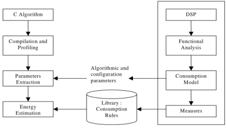
Our goal is to reduce the energy consumption of digital signal processing applications. A method for energy estimation is currently being developed, together with energy optimization strategies. The DSP’s energy consumption is estimated directly from the algorithm written in C. The complete methodology is sketched on figure 1.
Fig. 1. The Methodology
First step is to compile and profile the C algorithm. The algorithm is sliced in basic
blocks (a contiguous section of code with no loop and no branch [2]); specific
pa-rameters are extracted, such as the internal memory access rate, the number of proc-essing units used per cycle, the parallelism rate (provided that the DSP has parallel-ism capabilities), and the number of times a basic block is executed. Second step is to
C Algorithm Compilation and Profiling Parameters Extraction Energy Estimation Library : Consumption Rules DSP Functional Analysis Consumption Model Meausres Algorithmic and configuration parameters Preliminary work
estimate every basic block’s power consumption. The application’s overall energy consumption is finally computed.
The estimation model relies on a set of consumption rules, gathered in a library. In this paper, only the energy estimation model will be discussed, as well as the con-sumption rules’ determination and validation.
2.2 Functional Analysis
To actually build the library, a functional analysis of the targeted DSP is first per-formed. Non-consuming parts of the DSP are discarded (control registers of the DMA for instance, since they do not commute often enough).
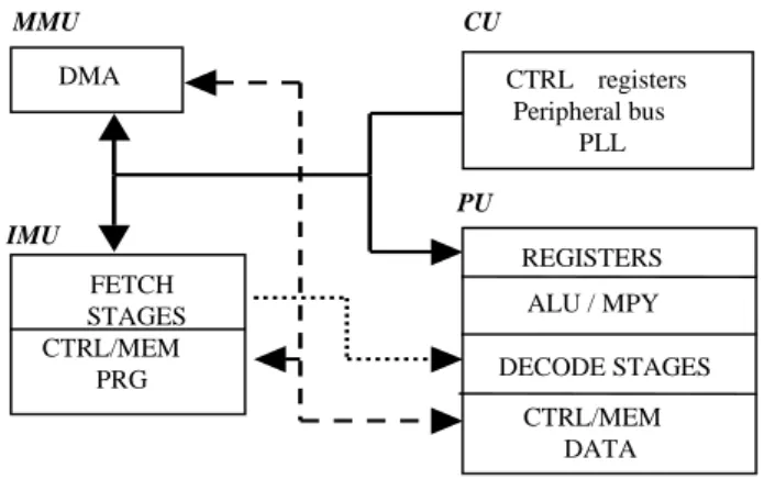
By adding or removing blocks or sub-blocks, the very general representation on figure 2 can be modified, depending on the targeted processor. In this model, 4 high-level blocks are exhibited: the CU block (Control Unit), the MMU (Memory Man-agement Unit), the IMU (Instructions ManMan-agement Unit) and the PU (Processing Unit). Each of them has several sub-blocks.
The functional diagram shows how blocks interact with each other. For instance, the DMA (Direct Memory Access) can generate an interaction between the MMU and PU if data are directly loaded from the external memory. An interaction exists be-tween the IMU and the PU for instructions are first fetched in the IMU, then executed in the PU. Interactions exist between the CU and every other block, since it contains the DSP’s control registers.
Fig. 2. Functional Diagram
The power consumption induced by every interaction on this diagram is investi-gated afterward. The next section presents a complete analysis for a real DSP.
DMA CTRL registers Peripheral bus PLL FETCH STAGES CTRL/MEM PRG REGISTERS ALU / MPY DECODE STAGES CTRL/MEM DATA PU MMU IMU CU
2.3 The TMS320C6201’s Study
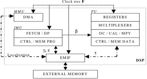
The TMS320C6201, one of the last generation Texas Instruments’ DSP, has a rela-tively complex architecture, since it has a deep pipeline (up to 11 stages), VLIW in-structions (256 bits inin-structions), parallelism capabilities (up to 8 inin-structions in par-allel), and an internal program memory that can be used in cache mode. Its functional diagram is presented in figure 3 (only inter-blocks interactions are shown).
Fig. 3. Functional Analysis for the TMS320C6201
The clock tree is represented as an external interaction to every block. The con-sumption it induces is rather high since 200MHz is the DSP’s nominal frequency.
The pipeline’s DECODE stage is broken in 2: the dispatching part (DP) is included in the IMU, and the instructions decoding (DC) remains in the PU. In this DSP indeed, decoding is actually done in the processing unit, whereas dispatching is realized in the fetch stage.
The EMIF (External Memory InterFace) tackles every external memory access for both instructions and data. This new block has its own interactions. The first one, to the IMU, is only activated when the CPU loads instructions from the external memory (in case of a cache miss for instance). The second, to the PU, is activated when data are loaded.
Although other interactions than those reported on this diagram may exist, they are not considered for they do not produce any significant enough power consumption.
The power consumption actually induced by every interaction depends on parame-ters from the algorithm. Configuration parameparame-ters are considered apart: they are the frequency (F), and the data mapping in memory. Regular algorithmic parameters are the average number of processing units used per cycle (β), the cache miss rate (γ), the in-external instructions (program) read rate (ε) and the in-external data access rate (τ).
In the following, every interaction will be considered to produce the consumption rules which are mathematical functions of the former parameters.
D M A F E T C H / D P C T R L / M E M P R G E M IF R E G IS T E R S M U L T IP L E X E R S D C / U A L / M P Y C T R L / M E M D A T A E X T E R N A L M E M O R Y IM U M M U P U C lo ck tree F L ocalizatio n β γ, ε τ D S P
3 Consumption Laws Determination
In this section, the energy consumption of every block in the functional diagram is determined. This consumption actually depends on the way a block interacts with each other (in this way, an interaction is said able to induce power consumption).
Several programs were used to stimulate independently every functional block. These programs (also called scenarios) are unbounded loops, written in assembly language, that excite only specific parts in the DSP. The branch at the end of the loop is negligible when the loop size is more than 4000 instructions. For every scenario, several configuration and algorithmic parameters were used. Each time, the energy consumption was measured and plotted on a set of charts from which the block’s con-sumption rule is eventually identified. The concon-sumption law for the block is eventually identified from the set of charts.
To know how much energy was consumed during a scenario, it is necessary to measure the average current consumed by the DSP’s core (ICORE) and the scenario’s execution time (TTOTAL). Given the core supply voltage (Vdd =2.5V), it is possible to determine the average total energy ETOTAL:
ETOTAL = ICORE * TTOTAL * Vdd (1)
Identically, it is possible to measure the energy consumed by a basic block EBB : EBB = ICORE * TEXE * Vdd (2) Where TEXE is the block’s execution time. Hence, to estimate the algorithm’s overall energy consumption, by adding up every basic block’s energy :
ETOTAL = Σ EBB (3)
In the following, consumption laws’ determination is demonstrated for the IMU (Instructions Management Unit) and the PU (Processing Unit).
3.1 The IMU’s Consumption Rules
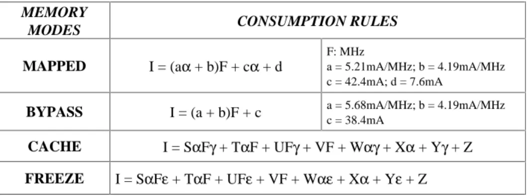
The IMU includes the fetch stage and the program memory with its controller. In the TMS320C6201, the program memory works in four modes. The first one is the MAPPED mode where all the instructions are in the internal program memory. The second is the CACHE mode, where external accesses are done whenever the instruc-tions are not in the cache (cache miss). The third is the FREEZE mode, similar to the CACHE mode but the cache is only read and never written. The last one is the BY-PASS mode, where all the instructions are read from external memory.
Table 1 shows the measured average current and energy consumed by the DSP’s core for one loop’s iteration. The results are identical for the CACHE and the FREEZE mode, since no cache miss was generated in this scenario (only CACHE mode appears in the table).
MEMORY MODE
FREQUENCY
CURRENT (mA)
ENERGY (µj)
MAPPED 1300 24.44 CACHE 1342 25.22 BYPASS 133MHz 795 120 MAPPED 1554 24.3 CACHE 1595 24.9 BYPASS 160MHz 948 237 MAPPED 1840 23 CACHE 1904 23.8 BYPASS 200MHz 1175 235
Table 1. Memory Modes Comparison
Obviously, the current is not the only parameter for comparing the TMS’s memory modes. Indeed, measured current is lower in BYPASS mode than in MAPPED (about –39%), but much more energy is used (at least +390%). Energy is the most important parameter, not only for embedded applications; however, it is necessary to measure currents to elaborate our consumption laws.
Since sub-blocks change with the memory mode, four rules have to be elaborated (the cache controller is only present in CACHE and FREEZE modes, for example). For each memory mode, a scenario was created to stimulate only the block we wanted. For every scenario, the PU (Processing Unit) was never excited. After several meas-urements for different algorithmic and configuration parameters’ values, a mathemati-cal function is sought that gives the consumption rule.
Table 2 presents the consumption rules for the 4 memory modes. MEMORY
MODES CONSUMPTION RULES
MAPPED I = (aα + b)F + cα + d
F: MHz
a = 5.21mA/MHz; b = 4.19mA/MHz c = 42.4mA; d = 7.6mA
BYPASS I = (a + b)F + c a = 5.68mA/MHz; b = 4.19mA/MHz
c = 38.4mA
CACHE I = SαFγ + TαF + UFγ + VF + Wαγ + Xα + Yγ + Z FREEZE I = SαFε + TαF + UFε + VF + Wαε + Xα + Yε + Z
For the CACHE and FREEZE mode, coefficients S, T, U, V, W, X, Y and Z de-pend on ε or γ ranges. The FREEZE mode was split in 2 depending on ε (ε≤25% or ε>25%). The CACHE mode was split in 3 depending on γ (γ<50%, 50%≤γ≤75%, γ>75%).
For these 2 modes, the consumption is constant if the parallelism rate (α) is greater or equal to 0.5 thus the current is estimated with the rules for γ or ε equals 0%.
3.2 Processing Unit Rules
Parameters involved in the PU’s consumption rule are the number of processing units per cycle (β) and the operating frequency (F). β equals 8 when all the processing units are used, 0 on the contrary. In this case, β is 8 times the parallelism rate α (which varies from 1 to 1/8). The consumption rule is [IPU : average current (mA)] :
IPU = aβF a=0.64mA/MHz; F: frequency (MHz) (4)
The data variations (in size and value) are not considered since their influence on power consumption is negligible for this DSP [5].
4 Application
In this section energy estimation is applied on a classical signal processing algorithm : a FIR16 filter. The TMS320C6201 is targeted. Firstly, we show how configuration and algorithmic parameters are extracted from the algorithm. Secondly, estimations and measures are compared to validate our model.
4.1 Parameters’ Extraction
The parameters we are extracting come from the former functional analysis for this particular DSP (see figure 3). For the IMU, every memory mode is investigated with γ and ε varying. The parallelism rate α gives the FETCH stage consumption. To calcu-late α, we count how many FP (Fetch Packets) and EP (Execute Packets) are used in the program, then we divide the number of EP by the number of FP; this ratio gives α.
Since the filter’s coefficients and input samples are mapped in the internal data memory, we simply have to consider β for the PU (Processing Unit). The number of processing units used in one iteration of the program is counted. Then it is divided by the number of processor cycles necessary to execute the iteration; this ratio gives β.
The application’s consumption is determined by adding up the contribution of every identified functional block (figure 3).
Table 2 compares measures and estimations for the MAPPED and BYPASS mode at the maximum DSP’s frequency (F=200MHz).
FIR 16 Global Estimate (µj) Measures (µj) Error (%) Mapped 105 104 0.96 Bypass 791 794 -0.38
Table 3. FIR16 Energy Estimations and Measures (in µj per iteration)
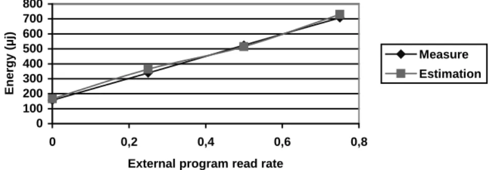
The energy consumption is estimated with an error lower than 1%. The following results are for the CACHE and FREEZE mode with γ and ε varying. Figure 4 presents estimations and measures in FREEZE mode for ε ranging from 0 to 75%.
Fig. 4. FIR16 Energy Estimations and Measures
The maximum error is less than 7.4%. It is greater than in MAPPED or BYPASS mode because the model complexity increases, and approximations made to determine the consumption rule are stronger.
Figure 5 presents the results in CACHE mode when γ varies from 0 to 100%. The maximum error in this mode is lower than 3.63%. In the very general case, es-timation is performed by adding up every basic block’s energy consumption (in our example, only one basic block was involved). For each basic block, parameters are extracted and energy estimated thanks to consumption rules. As stated before, the total energy is obtained this way (equation (3)).
0 100 200 300 400 500 600 700 800 0 0,2 0,4 0,6 0,8
External program read rate
Ene rgy ( µ j) Measure Estimation
0 200 400 600 800 1000 0 0,2 0,4 0,6 0,8 1 1,2 Cache miss rate
Ene rgy ( µ j) Measure Estimation
Fig. 5. FIR16 Energy Estimations and Measures
5 Conclusion
We propose a new approach to estimate the energy consumption of a DSP’s applica-tion. It relies on a set of rules that permit, given specific parameters extracted from the algorithm, to estimate the application’s energy consumption. In order to determine the set of consumption rules, a functional analysis of the DSP is first performed. The way interactions between functional blocks induce power consumption depends on several parameters which are clearly identified (configuration and algorithmic parameters). By running different scenario on the DSP, with different values for these parameters, a set of charts is obtained, from which the consumption rules are computed. The method was applied to a FIR 16 filter on a TMS320C6201 DSP. The difference between our estimations and measurements never exceeded 7.4%. Functional analysis appears a very efficient and straightforward method for energy optimization. Future works aim at the development of energy reduction strategies for high-level algorithmic transfor-mations.
References
1. J.M. Rabaey, M. Pedram "Low power design methodologies" Kluwer Academic Publishers 1996.
2. Vivek Tiwari, Sharad Malik, Andrew Wolfe "Power analysis of embedded software: a first step towards software power minimisation." IEEE Transactions on VLSI Systems, Decem-ber 1994.
3. Mike Tien-Chien-Lee, Vivek Tiwari, Sharad Malik and Masahiro Fujita "Power Analysis and Minimisation Techniques for Embedded DSP Software." IEEE Transactions on VLSI Sys-tems, Vol5, N°1, March 1997.
4. P. Vanoostende et al. "Issues in low power design for telecom" IEEE 1995 p 591-593. 5. J.Laurent, N. Julien, E. Martin " High Level power Estimation for DSP" in proceedings of
6. J.Laurent, N. Julien, E. Martin “High Level Power Analysis for Embedded DSP Software” Technical Committee on Computer Architecture Newsletter, January 2001, pages 41-46 http://computer.org/tab/tcca/NEWS/jan2001/index.html.
7. P.Laramie "Instruction level power analysis and low power design methodology of a micro-processor", Master Thesis, U.C. Berkeley.
8. C. Brandolese, W. Fornaciari, F. Salice, D. Sciuto “An Insrtuction-Level Functionality-Based Energy Estimation Model for 32-bits Microprocesseur” proceedings of Design Automation Conference 2000, pages 346-342