HAL Id: hal-01300833
https://hal.archives-ouvertes.fr/hal-01300833
Submitted on 11 Apr 2016
HAL is a multi-disciplinary open access
archive for the deposit and dissemination of
sci-entific research documents, whether they are
pub-lished or not. The documents may come from
teaching and research institutions in France or
abroad, or from public or private research centers.
L’archive ouverte pluridisciplinaire HAL, est
destinée au dépôt et à la diffusion de documents
scientifiques de niveau recherche, publiés ou non,
émanant des établissements d’enseignement et de
recherche français ou étrangers, des laboratoires
publics ou privés.
Index Expanded Beam Connectors
Sy Dat Le, Philippe Rochard, Jean-Baptiste Briand, Lionel Quétel, Sébastien
Claudot, Monique Thual
To cite this version:
Sy Dat Le, Philippe Rochard, Jean-Baptiste Briand, Lionel Quétel, Sébastien Claudot, et al..
Cou-pling Efficiency and Reflectance Analysis of Graded Index Expanded Beam Connectors. Journal of
Lightwave Technology, Institute of Electrical and Electronics Engineers (IEEE)/Optical Society of
America(OSA), 2016, 34 (9), pp.2092-2099. �10.1109/JLT.2016.2525804�. �hal-01300833�
Abstract—This article deals with coupling efficiency and reflectance analysis of graded-index expanded-beam connectors. We point out the best conditions to take advantage of expanded beam connectors for relaxing lateral offset tolerances without going down to critical angle misalignments tolerances. The influence of manufacturing defaults and coupling misalignments by lateral offset and tilt angle on coupling efficiency and reflectance are theoretical analyzed, investigated and compared to experimental results. The study explains an interesting reflectance of expanded beam connectors compared to standard single-mode fibers. We demonstrate and explain why we can both obtain high coupling efficiency and low reflectance.
Index Terms— Coupling efficiency, expanded beam, graded index fiber, optical coupling, optical connector, reflectance.
I. INTRODUCTION
UE to their very small mode field diameter (MFD), around 10 µm at telecommunication wavelength of 1550 nm, standard single mode fiber (SMF) connectors are very sensitive to contaminants, laser power [1], lateral and axial positioning tolerances. The idea to increase the beam at the fiber output to avoid these problems is not new, different methods have been proposed such as thermal diffusion of dopants [2][3], the use of lenses either discrete [4] or spliced to the SMF [5], for physical contact (PC) or free space connection, but it remains of great interest [6]. Free space connection has the advantage of not damaging the optical faces, but it is sensitive to fluid intrusion and reflections are complex to manage. In a previous work [7], we have proposed a physical contact connector easy to fabricate based on a graded index fiber (GIF) section spliced to a SMF that offers all the advantages of a large beam expansion (56 µ𝑚 of MFD), low insertion loss (IL), high return loss (RL) and low sensitivity to contaminants. We have demonstrated a good fit
Manuscript received December 09, 2015; revised January 25, 2016; accepted January 31, 2016. Date of publication Month Date, yyyy. This work was supported in part by the French government R&D funding within the RAPID CODEF project, under grant no. 132906103.
Sy Dat Le, Philippe Rochard, and Monique Thual, are with the CNRS UMR Foton, Université de Rennes 1, 6 rue de Kérampont, F-22305 Lannion, France. (e-mail: [email protected]).
Lionel Quétel and Jean Baptiste Briand are with IDIL Fibres Optiques, 21 rue Louis De Broglie 22300 Lannion, France. (e-mail: [email protected]).
Sébastien Claudot is with Souriau-Sunbank - Esterline ECT, RD323, 72470 Champagné, France. (e-mail: [email protected]).
Color versions of one or more of the figures in this paper are available online at http://ieeexplore.ieee.org.
Digital Object Identifier …
between theoretical and experimental evolution of the beam diameter, low IL (< 0.5 dB) at a wavelength of 1550 nm and low sensitivity to contaminants such as water, oil and dust. But the theoretical and principal of studies for neither IL nor RL have been presented.
In this paper we present a theoretical analysis of the coupling efficiency (which leads to IL) and reflectance (linked to the RL) of this kind of connectors based on GIF sections whose end face is either perpendicular or angled to fiber axis. Experimental results also will be presented to compare with theoretical studies.
For this study we benefit from very useful publications developed as soon as 1964 by H. Kogelnik on coupling of optical modes [8], on Gaussian beams propagation through optical systems [9][10], and by other authors on coupling of Gaussian beams [11] and their propagation in graded index media [5][12][13] with or without axial, lateral and angular misalignment.
The novelty of our present work consists first in the analysis of both coupling efficiency and reflectance with and without defaults, such as GIF section length default compared with the optimum one with offset and tilt, second we perform this analysis by two different methods. The first one is analytic and the second one is based on the beam propagation method (BPM) which allows to take into account the truncation of the beam by the cladding during its propagation in the GIF section. The aim is to try to point out the best conditions to achieve a high coupling efficiency and low reflectance.
In a first section we will present the principle of the expanded beam connector and the parameters studied in our analysis, and we will introduce the coupling efficiency and reflectance equations. In a second section we will present our calculations first by an analytical method and second by BPM. Then we will summary and discuss our theoretical results compared with our experimental ones on both misalignment and fabrication tolerances before conclusion.
II. PRINCIPLE AND THEORETICAL CONCEPTS A. Principle of the expanded beam connector studied
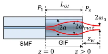
The expanded beam connector consists of introducing a micro-lens at the end of the SMF. For that purpose a GIF section is spliced to a SMF as shown in Fig.1. Thanks to the parabolic transverse index profile of the GIF section, the beam size 2𝜔(𝑧) and the radius of curvature of the wave front 𝑅(𝑧) of the Gaussian beam coming from the SMF has a periodic evolution along the optical axis z when propagating in a length
Coupling Efficiency and Reflectance Analysis
of Graded Index Expanded Beam Connectors
Sy Dat Le, Philippe Rochard, J.-B. Briand, Lionel Quétel, Sébastien Claudot, and Monique Thual
of GIF, 𝐿𝐺𝐼. The index profile is considered to be a perfect parabolic curve conforming to the relationship:
𝑛(𝑟) = 𝑛0(1 − ∆𝑟
2
𝑎2) (1),
where 𝑛0 is the central refractive index, ∆ is the relative index difference between 𝑛0 and 𝑛𝑐 (the refractive index of the GIF cladding) defined as ∆= (𝑛02− 𝑛𝑐2)/(2𝑛02), 𝑟 the radial position in relation to the optical axis and 𝑎 the core radius of the GIF. The numerical aperture (NA) is (𝑛02− 𝑛𝑐2)1/2= 𝑛0(2∆)1/2.
For an optimum 𝐿𝐺𝐼 referred as 𝐿𝐺𝐼𝑜𝑝𝑡, the beam size 2𝜔(𝑧) in the GIF is enlarged to a maximum 2𝜔𝑚𝑎𝑥. Then the beam size decreases in the GIF section. The value of 𝐿𝐺𝐼𝑜𝑝𝑡 depends on the GI refractive index profile and its core diameter. Defining the GIF parameter as 𝑔 = (2∆)1/2/𝑎, the optimal GIF length is given by 𝐿𝐺𝐼𝑜𝑝𝑡= 𝜋/(2𝑔) [14]. In this configuration, as the phase front is plane at the fiber end, the working distance, 𝑧𝑤, (see Fig. 1) is zero and the beam waist (2𝜔0) is equal to the maximum beam diameter (2𝜔𝑚𝑎𝑥). To produce the large beam connection, each ferule connector contains a GIF section with this length 𝐿𝐺𝐼𝑜𝑝𝑡 spliced to a SMF, so the total length of two GIF sections is 2 × 𝐿𝐺𝐼𝑜𝑝𝑡, as illustrated in Fig. 2. Since the fiber diameter remains 125 µm over the length of the micro-lens, it is suitable to be inserted in a standard connector ferule.
B. Coupling efficiency and Reflectance
We have analyzed the coupling efficiency and reflectance of this kind of connectors when offset and tilt are present in the system as shown in Fig. 3. The lateral offset 𝑥1and tilt 𝜃1 between the incident fundamental mode of SMF1 and the
optical axis of GIF1 are defined in the plane P1 (The plane P1
is perpendicular to GIF1 axis). The lateral offset 𝑥1+ and 𝜃1+ between the output beam 𝜓1+ of GIF2 and its axis, and the lateral offset 𝑥2 and 𝜃2 between GIF2 and SMF2 are defined in the plane P2, perpendicular to this axis. The lateral offset 𝑥3 and tilt 𝜃3 between the optical axis of GIF1 and that of GIF2 are defined in the plane P3 as can also be seen in Fig. 3.
Given that the SMFs are spliced to the GIFs and the GIFs are in contact in the connector, it is assumed that no axial gap is present between the fibers.
The coupling efficiency 𝜂𝑐𝑜𝑢𝑝 is defined as the fraction of power coupled from the incoming fundamental mode of SMF1, after propagation forward in a length 2 × 𝐿𝐺𝐼 of GIFs, to the fundamental mode of SMF2 at the reference plane P2.
It is given by 𝜂𝑐𝑜𝑢𝑝=
|∬−∞+∞𝜓1+.𝜓2∗ 𝑑𝑥𝑑𝑦|2 ∬−∞+∞𝜓1+.𝜓1+∗ 𝑑𝑥𝑑𝑦 ∬−∞+∞𝜓2.𝜓2∗ 𝑑𝑥𝑑𝑦
(2),
where 𝜓1+is the complex field of the beam coming from SMF1 expressed in the plane P2 after propagation in the GIF1 and
GIF2 and 𝜓2 the complex field of fundamental mode of SMF2 at the same plane P2, and asterisk denotes a complex
conjugate.
The reflectance 𝜂𝑟𝑒𝑓𝑙 is the fraction of power coupled at the plane P1 from the incoming fundamental mode of SMF1 after
propagating forward in a length 𝐿𝐺𝐼 of GIF1, reflecting at the GIF1 surface end (plane P3) and propagating backward in the
same length of GIF1 (complex field 𝜓1−), to the fundamental mode of SMF1 (complex field 𝜓1). It is given by
𝜂𝑟𝑒𝑓𝑙= |∬+∞𝜓1−.𝜓1∗ 𝑑𝑥𝑑𝑦 −∞ | 2 ∬ 𝜓1−.𝜓 1 −∗ 𝑑𝑥𝑑𝑦 ∬ 𝜓1.𝜓 1 ∗ 𝑑𝑥𝑑𝑦 +∞ −∞ +∞ −∞ (3). C. Analytical method
The complex amplitude of the input field 𝜓1 in general case of an offset 𝑥1 and a tilt 𝜃1 between SMF1 and GIF1 in relation to the optical axis is given by [8]:
𝜓1= (√𝜋2𝜔1 1) 1 2 𝑒𝑥𝑝 {−(𝑥−𝑥1)2 𝜔12 − 𝑗𝑘𝜃1(𝑥 − 𝑥1)} (4),
where 𝜔1 is the mode field radius and 𝑘 = 2𝜋𝑛0/𝜆 is the propagation constant in the media, 𝜆 is the wavelength of light in vacuum. In the case of beam propagation in vacuum, the vacuum constant 𝑘0= 2𝜋/𝜆 is used instead of the constant 𝑘. Note that the additional optical path leading to the phase shift (imaginary part in (4)) due to the tilt is approximated as 𝜃1(𝑥 − 𝑥1) by assuming tilt angle to be small.
The ABCD matrix of GIF is used to analytically characterize the propagation of a Gaussian beam in GIF1 and GIF2 [10]. The beam ray is calculated at the beam width defined at 1/𝑒2 of maximum intensity and determined by the height 𝑥 and the angle slope 𝜃 as
[𝑥𝜃] = [ cos(𝑔𝑧) sin (𝑔𝑧) 𝑔𝑛0 −𝑔𝑛0sin (𝑔𝑧) cos (𝑔𝑧) ] [𝑥𝜃1 1] (5).
We have also the 𝑞2 parameter at z position given by 𝑞2= 𝐴𝑞𝐶𝑞1+𝐵
1+𝐷 (6),
where 𝑞1 is the q-parameter at the input plane P1 [9]. It is
Fig. 1. Principle of the SMF-GIF micro-lens.
Fig. 3. Tilts and offsets in the connectors Fig. 2. Principle of the expanded beam connector.
given by 𝑞1= 𝑗𝜋𝜔12/λ (assuming an input beam from the SMF1 with a plane wave front). The beam size 𝜔1(𝑧) and the radius of phase front curvature 𝑅1(𝑧) are calculated from the complex 𝑞-parameter as 𝜔1(𝑧) = √−𝜋𝐼𝑚(1 𝑞𝜆 2 ⁄ ) (7), 𝑅1(𝑧) = 𝑅𝑒(1 𝑞1 2 ⁄ ) (8). The complex field at any plane along 𝑧-distance can be formed from 𝜔1(𝑧), 𝑅1(𝑧), offset 𝑥1, and a tilt 𝜃1. In this case at the plane P2, the complex field 𝜓1+ which has propagated forward (+) from an initial field 𝜓1 can be written as
𝜓1+= (√2𝜋𝜔1 1(𝑧)) 1 2 𝑒𝑥𝑝 {−(𝑥−𝑥1+)2 𝜔12(𝑧) − 𝑗𝑘 (𝑥−𝑥1+)2 2𝑅1(𝑧) − 𝑗𝑘𝜃1 +(𝑥 − 𝑥 1+)} (9), where 𝜔1(𝑧) and R1(z) are the beam radius and the radius of
phase front curvature of the Gaussian beam at the output plane P2 after a propagation of a distance z in GIF. 𝑥1+ and 𝜃1+ are the offset and tilt of the complex field 𝜓1+ with respect to optical axis of GIF2 as seen in Fig. 3.
By referring to optical axis of GIF2 and considering that the phase front curvature of complex field at one end of SMF2 is infinity, the complex field of 𝜓2 can be given by
𝜓2= (√2𝜋𝜔1 2) 1 2 𝑒𝑥𝑝 {−(𝑥−𝑥2)2 𝜔22 − 𝑗𝑘𝜃2(𝑥 − 𝑥2)} (10), where 𝜔2 is the beam radius of the Gaussian beam of SMF2 at the plane P2, 𝑥2 and 𝜃2 are the offset and tilt respectively between SMF2 and GIF2 optical axis.
The coupling efficiency of complex fields 𝜓1+ and 𝜓2 is then calculated by using (2). An analytical expression by using the Gaussian beam approximation [11] could also be applied to this case.
The study on coupling efficiency of expanded beam connectors deals with not only in the plane P2 but also in the
plane P3 between GIF1 and GIF2. In this case, we consider
that two Gaussian beams are injected in GIF1 and GIF2 from SMF1 and SMF2, respectively. At each input plane P1 and P2,
the SMF and GIF are positioned at different lateral positions and misalignment angles to examine beams coupling in the plane P3. The coupling efficiency is then calculated from two
complex fields 𝜓1+ and 𝜓2+ from two initial complex fields 𝜓1 and 𝜓2 by using the same (2) as above.
The expanded beam connectors experimentally reported in [7] have lower reflectance compared to SMF or multimode fibers. To understand this advantage of SMF-GIFs, the reflectance on GIF surface end of SMF-GIF connectors is theoretically investigated. The GIF-end surface is examined as a plane surface which can be either a perpendicular end or an angled end to GIF optical axis.
The beam rays after being reflected by the surface propagate backward to the input fiber. The reflected complex field 𝜓1− ("" denotes the backward) is illustrated as dash lines in Fig. 3. The reflectance is then obtained by using the integral equation for two complex fields 𝜓1− and 𝜓1. Referring to GIF1 optical axis, the complex field 𝜓1 is displaced of an offset 𝑥1
and tilted of an angle 𝜃1. The reflected field 𝜓1− is displaced by an offset 𝑥1− and a tilt 𝜃1− which are obtained by using (5), (6), and (7).
D. Beam Propagation Method
In order to understand beam truncation due to the GIF core-cladding boundary, the propagation of beam is numerically modelled by using beam propagation method (BPM) [12, 15, 16]. The propagation of light through GIFs can be simulated with arbitrary refractive index profiles. The intensity fields in 3D are calculated in order to understand the beam truncation.
The refractive index profile of GIF from (1) can be rewritten as 𝑛(𝑥, 𝑦) = 𝑛𝑐+ 𝛿𝑛(𝑥, 𝑦), where 𝛿𝑛(𝑥, 𝑦) = 𝑛0− 𝑛𝑐+ ∆(𝑥2+ 𝑦2)/𝑎2 is a small transverse index variation.
The complex field amplitude 𝜓1 at the input plane P1
(𝑧 = 0) can be expressed in (𝑥, 𝑦) coordinates as 𝜓1(𝑥, 𝑦, 0) = (√𝜋2𝜔1 1) 1 2 𝑒𝑥𝑝 {−(𝑥−𝑥1)2+(𝑦−𝑦1)2 𝜔12 −𝑗𝑘𝜃1𝑥(𝑥 − 𝑥1) − 𝑗𝑘𝜃1𝑦(𝑦 − 𝑦1)} (11), where 𝑥1, 𝑦1 are the offsets on 𝑥, 𝑦 axes, 𝜃1𝑥, 𝜃1𝑦 are the tilts of initial field with respect to optical axis of GIF1.
The complex field amplitude relating 𝜓1(𝑥, 𝑦, 𝑧) to 𝜓1(𝑥, 𝑦, 0) can be implemented by the fast Fourier transform (FFT) and inverse FFT (IFFT) algorithms in BPM method. The field is sampled on a 𝑀 × 𝑀 computational grid of a window dimension 𝐿. The sampling interval on spatial domain is ∆𝑥 = ∆𝑦 = 𝐿/𝑀. In spectral domain of (𝑓𝑥, 𝑓𝑦) coordinates, the field is also sampled by FFT with an interval of ∆𝑓𝑥= ∆𝑓𝑦= 2𝜋/𝐿 of a spectral dimension 2𝜋𝑀/𝐿. The total length of the GIF is split into a number of small ∆𝑧 distances. Propagation is readily handled in the spatial and spectral domains using FFT and IFFT for a small step of ∆𝑧.
The field amplitude 𝜓(𝑥, 𝑦, ∆𝑧) at a small distance of ∆𝑧 is obtained from the well-known Helmholtz equation. With a small index variation 𝛿𝑛, it can be approximately written as
𝜓(𝑥, 𝑦, 𝑧 + ∆𝑧) ≅ 𝑒𝑥𝑝(𝐷̂∆𝑧)𝑒𝑥𝑝(𝑆̂∆𝑧)𝜓(𝑥, 𝑦, 𝑧) (12). where 𝐷̂ and 𝑆̂ are linear differential operator and space-dependent operator, respectively. Here, 𝐷̂ and 𝑆̂ are noncommuting operators and they are assumed to be z-independent. The first operator of (12) is the propagation operator. It considers the effect of diffraction between two adjacent planes 𝑧 and 𝑧 + ∆𝑧. Its expression in spectral domain is
𝐹𝐷= 𝐹𝐹𝑇[𝑒𝑥𝑝(𝐷̂∆𝑧)] = 𝑒𝑥𝑝 [𝑖(𝑘𝑥2+ 𝑘𝑦2)2𝑘𝑛(𝑥,𝑦)∆𝑧 ] (13), where 𝑘𝑥= 2𝜋𝑓𝑥 and 𝑘𝑦= 2𝜋𝑓𝑦 are the spatial frequencies. The rest of (12) is expressed in spectral domain by FFT as 𝐹𝑆= 𝐹𝐹𝑇{𝑒𝑥𝑝(𝑆̂∆𝑧)𝜓(𝑥, 𝑦, 𝑧)}
= 𝐹𝐹𝑇{𝑒𝑥𝑝(−𝑖𝑘𝛿𝑛(𝑥, 𝑦))𝜓(𝑥, 𝑦, 𝑧)} (14). The field amplitude after propagating a single step ∆𝑧 is then computed with the well-known IFFT algorithm
𝜓(𝑥, 𝑦, ∆𝑧) = 𝐼𝐹𝐹𝑇{𝐹𝐷. 𝐹𝑆} (15). The coupling efficiency and the return losses are obtained by applying an integration between two fields using (2) and (3) as in the above discussion. In the calculation of beam
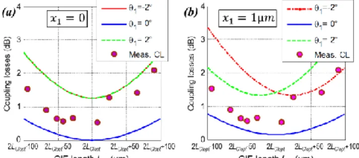
Fig. 6. (a) Misalignment between two SMF-GIF connectors at plane P3. CL
of two 55 µm SMF-GIF connectors with respect to (b) lateral offsets and (c) angular misalignments at plane P3.
propagation in a GIF, it should take into account the boundary condition of refractive index profile. The beam truncation is not only affected by the refractive index difference of core-cladding boundary but also that of core-cladding-air border.
III. RESULTS AND DISCUSSION
In order to confirm theoretical studies, the SMF-GIFs are fabricated with the GIF length around 𝐿𝐺𝐼𝑜𝑝𝑡 defined in (4). Fig. 4a illustrates the evolution of beam waist and working distance of the SMF-GIFs with the variation of GIF length 𝐿𝐺𝐼 at a wavelength of 1550 nm. The analytic and BPM calculations present nearly the same evolution. The maximum theoretical beam waist is about 57 µm for both calculation methods. The calculation also proves that at the GIF length of 𝐿𝐺𝐼𝑜𝑝𝑡, the beam waist is largest and the working distance is null. The measured MFD with respect to the GIF length compared with theoretical calculation is presented in Fig. 4b. The measurement shows in fact that the MFD is slightly smaller than theoretical calculation. The maximum MFD is measured to be 55µm. The beam truncation due to cladding-core boundary may cause the beam size reduction [17].
The coupling loss (CL) and the return loss (RL) are theoretically and experimentally investigated. For a given MFD of GIF1 and GIF2, they depend on the relative positions between SMF1 and GIF1, between GIF1 and GIF2, and between GIF2 and SMF2, and fiber surface end designs. We will consider the case of identical MFD of GIF1 and GIF2.
A. Misalignment coupling tolerances
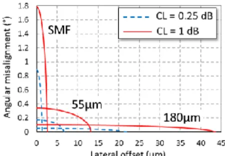
Firstly, coupling loss of two identical Gaussian beams with identical MFD is analytically calculated. Since the MFDs are identical the optimum CL is 0 dB if no air gap is present. However, it increases as a function of lateral offset and angular misalignment between the two Gaussian beams depending on the MFD. In fact, the larger MFD, the better lateral tolerances we have. However, larger MFD cause angular sensitivity. The positional tolerances corresponds to the lateral offset and angular misalignment that lead to an excess loss compared to the optimum. Fig. 5 gives a comparison of positional tolerances at 1 dB and 0.25 dB excess loss for the case of coupling two SMFs (2𝜔1~10.4 µm at 1550 nm) and the case of larger Gaussian beams (2𝜔1= 55 µm and 2𝜔1= 180 µm at 1550 nm). For 1 dB CL (solid or red curves), 55-µm-Gaussian beams and 180-µm-Gaussian beams taking the advantage of larger beams have significant lateral-offsets of about 13 µm and 43 µm, respectively. Angular misalignment of 55-µm-Gaussian beams
however is critical to 0.35° compared to 1.8° of SMFs. The theoretical calculation shows that expanded-beam connectors should not have an MFD larger than 180 µm. This ensures that CL not exceed 1 dB due to a crucial angle (0.1°), which is the mechanical limitation of standard optical connector fabrication.
Keeping in mind the above theoretical coupling calculation of two Gaussian beams, the 55-µm SMF-GIF connectors are now taken into account. The input beam from the SMF1 is expanded to its maximum at 𝐿𝐺𝐼𝑜𝑝𝑡 before converging at the plane P2. The maximum beam-size of this type of connectors
takes place at the plane P3. It means that at the plane P3 the
connectors may have good lateral tolerances but they also may suffer angular sensitivity. Misalignments at the plane P3 is
examined. In this case, defaults at the plane P1 and P2 are
neglected (Fig. 6a). The Gaussian beam from SMF1 propagates through GIF1 before being coupled into GIF2, then to SMF2. CL integral calculation is applied at the plane P2
between arriving complex field 𝜓1+ and a Gaussian field 𝜓2+ of SMF2. Figs. 6b and 6c present CL with respect to lateral offsets and angular misalignments. This coupling simulation of two SMF-GIFs is in accord with the coupling of two Gaussian beams as presented previously in Fig. 5. For example, CL = 1 dB if 𝑥3= 13 µ𝑚 and 𝜃3= 0° (Fig. 6a); or if 𝑥3= 0 µ𝑚 and 𝜃3= 0.34° (Fig. 6b). CL tolerances of 55 µm connectors were measured with the help of a refractive index liquid to avoid reflection losses. The normalized CLs agree well with the theoretical simulation as seen in Fig. 6.
Fig. 5. Coupling tolerances of two Gaussian beams with lateral offset and angular misalignment. Solid or red curves correspond to 1 dB of CL and dash or blue curves correspond to 0.25 dB of CL.
Fig. 4. (a) Analytical and BPM calculation of MFD, and (b) measured MFD of fabricated SMF-GIF connectors compared with theoretical calculation.
B. Fabrication defaults
CL is then investigated with respect to total GIF lengths (GIF1 + GIF2) relating to 2 × 𝐿𝐺𝐼𝑜𝑝𝑡 with lateral and angular defaults due to the fact of fabrication at the plane P1 (between
SMF1 and GIF1) and at the plane P2 (between SMF2 and
GIF2), assuming that misalignments at the plane P3 are
ignored (𝑥3= 0 and 𝜃3= 0°), see Fig. 3. Let’s start with a case of no default at the plane P2 (𝑥2= 0 and 𝜃2= 0°). Reminding that although there is no default at the plane P2, the
arrived field 𝜓1+ still can be misaligned with SMF2 due to input defaults at the plane P1. Fig. 7 presents CL regarding to
total GIF lengths 2 × 𝐿𝐺𝐼 (GIF1+GIF2) as respect to 2 × 𝐿𝐺𝐼𝑜𝑝𝑡 relating to different offsets 𝑥1 and different tilts 𝜃1 as well as measured CLs. Here, the measured CLs were taken for faultless expectation of fabrication. The blue curve in Fig. 7a presents the ideal case if 𝑥1= 0 and 𝜃1= 0°. When SMF1 and GIF1 are concentrically spliced, CL increases with tilts but its variation is identical for the same absolute tilts. As seen in Fig. 7a, the solid red curve (𝜃1= −2°) and the dash green curve (𝜃1= 2°) are overlapped. Fig. 7b is an example of CL with an offset 𝑥1= 1 µ𝑚 for different tilts. For a given 2 × 𝐿𝐺𝐼, CLs are different for different tilts even if tilts are the same absolute value. This could explain the scattering in CL measurement of SMF-GIFs because of unexpected defaults.
CL is now examined with a fixed angular tilt but the lateral offset is varied. In this case, the splice between GIF2 and SMF2 is also assumed to be perfect (𝑥2= 0 and 𝜃2= 0°). Fig. 8 shows CL regarding to total GIF lengths (GIF1+GIF2 for different lateral offsets 𝑥1, for 𝜃1= 0° (Fig. 8a), and for 𝜃1= 1° (Fig. 8b). The previously measured CLs in Fig. 7 are also reproduced in Fig. 8. In the case of 𝜃1= 0°, CL increases with the increment of lateral offset 𝑥1.
However at the minimum CLs, the total GIF length is always equal to 2 × 𝐿𝐺𝐼𝑜𝑝𝑡. In the perfect case (offsets and tilts are zeros at all planes), CL is null at the GIF length of 2 × 𝐿𝐺𝐼𝑜𝑝𝑡 as the minimum point on the blue curve in Fig. 8a. Moreover, this curve points out that the fabrication process is very tolerant with respect to a default in LGI length compared
to the optimum one, 𝐿𝐺𝐼𝑜𝑝𝑡. As can be seen on Fig. 8a, an error of ±50 µ𝑚 (very easy to achieve) compared with 𝐿𝐺𝐼𝑜𝑝𝑡 leads to less than 0.2 dB excess loss. However, CL increases to about 0.3 dB when SMF1 and GIF1 are tilted of
1° as seen in Fig. 8b. The offset increase leads to increment of CL. In the case of angular default presence, the minimum CL occurs at a shorter GIF length than 2 × 𝐿𝐺𝐼𝑜𝑝𝑡 if 𝑥1𝜃1> 0 (Fig. 8b) and at longer GIF length than 2 × 𝐿𝐺𝐼𝑜𝑝𝑡 if 𝑥1𝜃1< 0. That is why, for a given GIF length, CL varies quite fast for different offsets in the case of tilt existence.
Defaults at the input (between SMF1 and GIF1) can be fortunately corrected by defaults at the plane P2 between GIF2
and SMF2. The input defaults can be compensated or not depending on the relative position between GIF2 and SMF2. With input defaults, the beam arriving at the plane P2 is
absolutely off axis as seen in Fig. 9a for an example of 𝑥1= 3 µ𝑚 and 𝜃1= −10°. However, despite the imperfection at the input, CL can still be diminished if defaults at the plane P2 counterbalance to those at the plane P1. This corresponds to
the field with the dotted green curve which is overlapped with the arriving field in red curve (Fig 9b). On the contrary, CL increases due to misalignment between the arriving field 𝜓1+ and the SMF2 field at the plane P2 (the dash green and solid
green curves in Fig 9b, for examples).
Fig. 10 illustrates CL for both cases of default correction and of CL increment due to defaults between GIF2 and SMF2. The example is for input offset default 𝑥1= 2 µ𝑚 and angular default 𝜃1= 2°. If there is no default between GIF2 and SMF2, minimum CL is equal to 1.6 dB. CL can be canceled if defaults at the plane P2 are opposite to the input defaults. Here,
if 𝑥2= −2 µ𝑚 and 𝜃2= −2°, the CL is returned to 0 dB (blue curve). However, if defaults at the plane P2 are the same
signs with the inputs, CL considerably increases to 6.8 dB.
Fig. 7. Coupling losses with respect to total GIF lengths relating to 2 × 𝐿𝐺𝐼𝑜𝑝𝑡 for a fixed offset with different angular misalignments at the
input: (a) when SMF1 and GIF1 are concentric (𝑥1= 0) and (b) when SMF1 and GIF1 is 1 µ𝑚 off axis.
Fig. 9. (a) Beam ray propagation in GIF section with an input offset and a tilt, and (b) field arrives at the plane P2 (red curve) and SMF2 field without
default (green solid curve), with positive defaults (dash red curve), and with negative defaults (dotted green curve).
Fig. 8. Coupling losses with respect to total GIF lengths relating to 2 × 𝐿𝐺𝐼𝑜𝑝𝑡 for a fixed tilt with different lateral offsets at the input: (a) for the case of 𝜃1= 0°, and (b) for the case of 𝜃1= 1°.
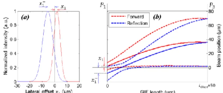
Fig. 12. An example of beam rays reflected at the GIF end surface return to SMF at the plane P1: (a) normalized field intensity of initial beam and
reflected beam at the plane P1 and (b) forward (red curves) and reflected
(blue curves) beam propagations in GIF section.
Fig. 13. RL with angled end face relating to surface angle φ of SMF and 55 µm SMF-GIF in comparison: (a) SMF and (b) 55 µm SMF-GIF.
C. Return losses
The reflectance is studied on the GIF1 surface end in contact with air, while the other end is spliced to the SMF1. Along GIF section, beam rays do not propagate parallel to the optical axis but progressively deviate by successive refractions in the parabolic transverse index profile. Reflected rays therefore are bent. In the ideal case of no default between SMF1 and GIF1 and if GIF length equals to 𝐿𝐺𝐼𝑜𝑝𝑡 and if GIF surface is flat and perpendicular to optical axis, the reflected rays will be firstly reflected parallel to optical axis then converged into the SMF1. In this case, the return beam is perfectly coupled back to SMF1. In any other way, this leads to a bad coupling back to the input SMF1. This explains why the reflectance of SMF-GIF is as low, compared to standard SMFs or multimode fibers, as will be shown below.
Fig. 11 shows calculatedRLs for different 𝐿𝐺𝐼 with an air-gap end perpendicular to the optical axis. The fabricated SMF-GIF connectors with faultless expectation were measured and also shown in both Fig. 11a and Fig. 11b. RL is calculated by taking into account the Fresnel reflection at the GIF1 surface end and loss by re-coupling the return beam into SMF1. The case in Fig. 11a, no lateral offset between SMF1 and GIF1 is considered, but angular misalignment is taken into account. RL varies depending on 𝐿𝐺𝐼, but it remains the same for all beams deriving from the input with the same absolute angle (𝜃1 = −2° and 𝜃1 = 2° as an example in Fig. 11a). It will be different if an offset appears. Fig 11b shows RL for an example of 1-µm offset between the SMF1 and GIF1. RL varies considerably in regard to 𝐿𝐺𝐼 when beam is angled. However, at the optimal length 𝐿𝐺𝐼𝑜𝑝𝑡, for a given offset 𝑥1, RL is independent to tilts. This can be seen as the intersection of three curves in Fig. 11b. For this example, RL is equal to 15.34 dB referred to 14.7 dB of RL at SMF surface.
In the case of RL, the lateral offset dependence is more critical compare to the angular misalignment (assuming that the GIF surface-end is perpendicular to the optical axis). As shown in Fig. 12, if the input offset is 𝑥1, the spot, where return chief ray arrives back at the input plane P1, depends on
the GIF length but will suffer an offset far from SMF1 center of about 2𝑥1. So offset defaults always lead to an increment of RL. The tilt of the return beam might be different from the input tilt 𝜃1 but they provide a good counterbalance to each other. So RL is less sensitive to input tilt. As seen in Fig. 12b, the input beam chief ray (red solid curve) launches in GIF at the beginning position above the optical axis (black horizon solid line). Therefore, the offset 𝑥1 is positive (𝑥1> 0). However, the return chief ray (blue solid curve) arrives at the plane P1 with a negative offset (𝑥1−< 0). The center of the return field and the SMF1 axis are distant from each other of |𝑥1| + |𝑥1−| as seen in Fig 12a.
RL of SMF-GIF connectors is now considered with angled surface end, which is at an angle 𝜑 to the normal to the fiber axis as seen in Fig. 13. The theoretical calculation of RL is implemented in the case of air-gap reflection. Theoretical RL of SMFs against surface angles is plotted in Fig. 13a and it is recalled in Fig. 13b as a reference for theoretical RL of 55 µm SMF-GIFs. For SMF, at the typical angle 𝜑 = 8°, theoretical RL is about 53 dB. For 55 µm SMF-GIF, we consider there is no fabrication default, neither GIF length (𝐿𝐺𝐼= 𝐿𝐺𝐼𝑜𝑝𝑡) nor input default at the input plane P1 (𝑥1= 0 and 𝜃1= 0°). In this case, any angle at surface end of SMF-GIFs always leads to a good RL (high RL) compared to SMFs one. Indeed, in the case of no input default, the chief ray of beam after being
Fig. 11. RL of SMF-GIF to air-gap with respect to LGI for different angular
misalignments and different lateral offsets: (a) 𝑥1= 0 and (b) 𝑥1= 1µ𝑚.
Fig. 10. Coupling loss correction of input defaults for the case of 𝑥1= 2 µ𝑚
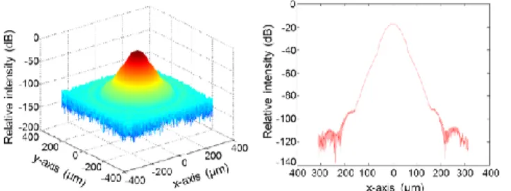
Fig. 14. Beam perturbation after propagating through GIF section. 2𝜔𝑚𝑎𝑥= 55 µ𝑚, 2𝑎 = 100 µ𝑚, 𝜌 = 0.55.
reflected at the GIF end is tilted from the fiber axis of an angle 2𝜑. This tilt causes lateral and angular misalignments between the reflected beam and SMF core. It leads to a significant increase of RL with the surface angle 𝜑 of the SMF-GIF compared with the SMF one as illustrated in both Fig. 13a and Fig. 13b. For example, if the surface angle 𝜑 = 1.6°, RL of an angled SMF-GIF is as high as 100 dB compared to 16.6 dB of 1.6°-angled SMF. This could explain the scattering in RL measurements shown in Fig. 11.
Above calculations of CL and RL are investigated by both analytical method and BPM method. The calculations show that both methods almost give the same results if the maximum beam size diameter (2𝜔𝑚𝑎𝑥) of beam in GIF is less than fiber core-radius 𝑎. In other words, if the ratio 𝜌 = 𝜔𝑚𝑎𝑥/𝑎 is less than 0.5 typically [18]. However, if the maximum beam size 2𝜔𝑚𝑎𝑥 exceeds the core radius or 𝜌 ≥ 0.5, the beam will be perturbed during propagating in GIF. This perturbation leads to somewhat differences between two methods. The larger ratio 𝜌, the more different in results we have. This can be explained by beam truncation during propagation in GIF as we can see in Fig. 14. The analytical method is simple and fast. Nevertheless, the BPM method is needed when doing investigation for large beams (𝜌 ≥ 0.5) to take into account perturbation.
In summary from the above discussion, defaults at the input plane P1 or angled surface end of SMF-GIFs always lead to a
low reflectance. Good RLs hence can be obtained. Defaults at the input plane P1 and at the output one P2 can give a good
coupling efficiency in transmission (low CL) if these defaults compensate each other.
IV. CONCLUSION
We have theoretically analyzed and experimentally demonstrated the coupling losses and return losses of GIF-based expanded-beam connectors. We have studied the influence on coupling losses of misalignment positioning and SMF-GIF fabrication defaults. We have pointed out the interest to expand the beam up to a certain limit to relax sensitivity of connectors to lateral offset without decreasing too much the tolerance to angular misalignment. A lateral offset of 2.5 µm leads to 1 dB excess CL for SMF connectors whereas it is relaxed to 13 µm and 43 µm in a connection with 55 µm and with 180 µm Gaussian beams, respectively. But it shouldn’t be larger than 180 µm to ensure that excess CL not exceed 1 dB due to critical angle of 0.1° (1.8° for SMFs) which is the mechanical limitation of standard optical
connector fabrication. Then we have studied the CL and RL results with fabrication defaults such as a 𝐿𝐺𝐼 length different to the optimum one with offset and tilt between SMFs and GIFs. We have pointed out that the fabrication process of SMF-GIF is very tolerant to an error in GIF length since an error of ±50 µm leads to less than 0.2 dB excess loss and it remains very tolerant even in the presence of lateral offsets and tilts between SMF and GIF. Moreover we have highlighted the interest of SMF-GIF connectors to improve the RL even with non-angled end face compared to SMF. And an only 1° angled surface end of SMF-GIF leads to the same RL of 53 dB as an 8° angled SMF face. And finally, in this work we have demonstrated and explained why we can both obtain high coupling efficiency and low reflectance with this SMF-GIF technology in expanded-beam connector fabrication.
REFERENCES
[1] D. S. Kokkinos, C. Saravanos, W. Stanford, W. Wang, and Y. Hua, “SC/APC fiber optic connectors connected and disconnected under high optical power,” presented at the Optical Fiber Communication Conf. (OFC), Anaheim, C.A., US, 2006, paper NTuA5.
[2] K. Shiraishi, Y. Aizawa, and S. Kawakami, “Beam expanding fiber using thermal diffusion of the dopant”, J. Lightw. Technol., vol. 8, no. 8, pp. 1151-1161, August 1990.
[3] G. S. Kliros and P. C. Divari, “Coupling characteristics of laser diodes to high numerical aperture thermally expanded core fibers”, J. Mater Sci:
Matter Electron, vol. 20, sup. 1, pp. 59-62, January 2009.
[4] A. Nicia, “Lens coupling in fiber-optics devices: efficient limits”,
Applied Optics, vol. 20, no. 18, pp. 3136-3145, September 1981.
[5] W. L. Emkey and C. A. Jack, “Analysis and evaluation of graded-Index fiber-lenses”, J. of Lightw. Technol., vol. 5, no. 9, September 1987. [6] D. Childers, M. Hughes, S. Lutz, and T. Satake, “Design and
performance of expanded beam, multi-fiber connectors”, presented at the Optical Fiber Communication Conf. (OFC), Los Angeles, C.A., US 2015, paper ThC1, Invited paper.
[7] S. D. Le, M. Gadonna, M. Thual, L. Quetel, J.-F. Riboulet, V. Metzger, D. Parker, A. Philippe, and S. Claudot, “Reliable expanded beam connector compliant with single-mode fiber transmission at 10 Gbit/s”, presented at the Optical Fiber Communication Conf. (OFC), Los Angeles, CA, US, 2015, paper W4B.5.
[8] H. Kogelnik, “Coupling and conversion coefficients for optical modes,” in Proceeding Symposium Quasi-Optics, vol. 14, pp. 333-347, 1964. [9] H. Koglenik, “On the propagation of Gaussian beams of light through
lenslike media including those with loss or gain variation”, Applied
Optics, vol. 4, no. 12, pp. 1562-1569, December 1965.
[10] H. Kogelnik and T. Li, “Laser beams and resonators”, Applied Optics, vol. 5, no.10, pp. 1550-1567, October 1966.
[11] M. Saruwatari and K. Nawata, “Semiconductor laser to single-mode fiber coupler”, Applied Optics, vol. 18, no. 11, pp. 1847-1856, 1979. [12] M. D. Feit and J. A. Fleck, “Light propagation in graded-index optical
fibers,” Applied Optics, vol. 17, no. 24, pp. 3990–3998, 1978.
[13] J. Alda and G. D. Boreman, “On-axis and off-axis propagation of Gaussian beams in gradient index media”, Applied Optics, vol. 29, no. 19, July 1990.
[14] M. Thual, P. Rochard, P. Chanclou, L. Quetel, and C. van Trigt, “Contribution to research on micro-lensed fibers for modes coupling,”
Fiber and Integrated Optics, vol. 27, no. 6, pp. 532-541, 2008.
[15] J. Van Roey, J. Van der Donk, and P. E. Lagasse, “Beam-propagation method: Analysis and assessment,” J. Opt. Soc. Amer., vol. 71, no. 7, pp. 803–810, July 1981.
[16] D. Lorenser, X. Yang, and D. Sampson, “Accurate modeling and design of graded-index fiber probes for optical coherence tomography using the beam propagation method”, IEEE Photonics Journal, vol. 5, no. 2, pp. 3900015-3900015, 2013.
[17] M. Thual, D. Malarde, B. Abhervé-Guégen, P. Rochard, and P. Chanclou, “Truncated gaussian beams through microlenses based on a graded-index section,” Optical Engineering, vol. 46, no. 1, pp. 015402-015402, 2007.