ℓ1-Adapted Non Separable Vector Lifting Schemes For Stereo Image Coding

ℓ

-ADAPTED NON SEPARABLE VECTOR LIFTING SCHEMES FOR STEREO IMAGE

CODING

M. Kaaniche

_{, B. Pesquet-Popescu}

_{and J.- C. Pesquet}

1

Telecom ParisTech, Signal and Image Proc. Dept. 37-39, rue Dareau, 75014 Paris, France mounir.kaaniche@telecom-paristech.fr beatrice.pesquet@telecom-paristech.fr

2

Universit´e Paris-Est, LIGM and UMR-CNRS 8049,

Champs-sur-Marne, 77454 Marne-la-Vall´ee, France jean-christophe.pesquet@univ-paris-est.fr

ABSTRACT

Due to the great interest of stereo images in several applications, it becomes mandatory to improve the efficiency of existing coding techniques. For this purpose, many research works have been devel-oped. The basic idea behind most of the reported methods consists of applying an inter-view prediction via the estimated disparity map followed by a separable wavelet transform. In this paper, we pro-pose to use a two-dimensional non separable decomposition based on the concept of vector lifting scheme. Furthermore, we focus on the optimization of all the lifting operators employed with the left and right images. Experimental results carried out on different stereo im-ages show the benefits which can be drawn from the proposed coding method.

Index Terms— Stereo image coding, disparity estimation, vec-tor lifting schemes, non separable transforms, adaptive transforms.

1. INTRODUCTION

Recent advances in acquisition and display technologies have con-tributed to a widespread usage of stereo images. These data corre-spond to 2 views, called left and right images, obtained by record-ing the same scene from two slightly different positions. One of the main advantages of these images consists of providing a three-dimensional perception to the users. Such a 3-D representation en-ables various functionalities like 3DTV, telepresence in videocon-ferences [1], computer vision and remote sensing. The increasing demand in stereo images have motivated many researchers to design efficient compression techniques for both storage and transmission purposes. A straightforward approach consists of separately cod-ing each image by uscod-ing existcod-ing still image coders. However, this method is not so efficient since the images are often highly corre-lated. Therefore, more efficient coding schemes have been designed to take into account the inter-image redundancies [2]. The state-of-the-art coding approach is a combination of inter-view prediction and transform coding. More precisely, the generic stereo image cod-ing scheme involves three steps. In the first step, one image (say the left one) is selected as a reference image, and the other image (the right one) is selected as a target image. After that, the dis-parity map between the right and the left images is estimated [3]. In the second step, the target image is predicted from the reference one along the disparity field, and the difference between the original target image and the predicted one, called residual image, is gener-ated. Finally, the reference image, the residual one and the disparity map are encoded. Generally, the disparity map is losslessly encoded using DPCM with an entropy coder whereas the residual and the reference images are encoded in different transform domains.

Pi-oneering techniques have been developed for the Discrete Cosine Transform [4, 5]. However, a great attention was paid to the wavelet transform domain to achieve the quality scalability and guarantee a lossy-to-lossless reconstruction [6, 7]. To this end, lifting schemes have been already used to encode the reference and the residual im-ages [7]. In a recent work [8], an adaptive lifting scheme is also presented. The direction of prediction is selected according to the local horizontal and vertical gradient information of the reference image. While this approach can achieve good results in terms of bi-trate, it is not efficient in a lossy coding context (especially at low bit rate) since it is very sensitive to the quality of the reference image. In [9], the disparity map and the residual image are generated by ap-plying a bandlet transform [10] to the left and the right images. In [11], a hybrid coding scheme is designed where DCT is employed for the best matching blocks and the Haar wavelet transform for the occluded ones. Recently, we have proposed a novel approach based on the Vector Lifting Schemes (VLS) [12]. It consists of coding the reference image in intra mode whereas the other image is coded ac-cording to a hybrid mode driven by the estimated disparity map. Its main feature is that it does not explicitly generate a residual image, but two compact multiresolution representations of the left and right images. We should note that the proposed joint multiscale decompo-sition is handled in a separable way by cascading one dimensional (1D) VLS along the horizontal direction, then along the vertical one. However, it is well known that such a separable processing may not be well-suited for images with edges which are neither horizontal nor vertical. To overcome this drawback, some works on still image compression have been devoted to the development of 2D non sepa-rable lifting schemes in order to offer more flexibility in the design of the transform [13, 14, 15].

Due to the advantages of using non separable structures as shown in [15], we propose to perform the joint coding of the stereo image by adopting an extension of the previous VLS structure to 2D Non Separable schemes. The resulting decomposition will be denoted in what follows by NS-VLS. Another objective of this work is to de-sign adaptive decomposition, well adapted to the characteristics of the images, through an optimization of all the filters used with the reference and the target images. While the proposed design strategy is inspired from our recent nonsmooth optimization technique used for still image coding [16], it is worth pointing out that this paper aims at extending this technique to the context of stereo image cod-ing.

The remainder of this paper is organized as follows. In Sec. 2, we present the principle of the considered NS-VLS decomposition. The proposed optimization strategy is described in Sec. 3. Finally, in Sec. 4, experimental results are given and some conclusions are

drawn in Sec. 5.

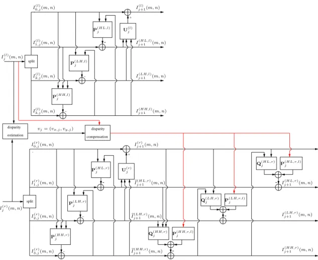
2. 2D NS-VLS STRUCTURE

Let I(l) and I(r) denote the left and right images to be coded. At each resolution level j and each pixel location (m, n), the ap-proximation coefficient of the left image I_j(l) (resp. right image I_j(r)) has four polyphase components I0,j(l)(m, n) = I

(l) j (2m, 2n), I1,j(l)(m, n) = I (l) j (2m, 2n + 1), I (l) 2,j(m, n) = I (l) j (2m + 1, 2n), and I_3,j(l)(m, n) = I_j(l)(2m + 1, 2n + 1) (resp. I_0,j(r)(m, n) = Ij(r)(2m, 2n), I (r) 1,j(m, n) = I (r) j (2m, 2n + 1), I (r) 2,j(m, n) = I_j(r)(2m + 1, 2n), and I_3,j(r)(m, n) = I_j(r)(2m + 1, 2n + 1)). The proposed analysis NS-VLS structure is shown in Fig. 1. As men-tioned before, the reference image I(l)_{is generally encoded in intra} mode. Thus, it can be seen that a non separable structure, com-prising three prediction steps and an update step, is employed to generate the diagonal detail coefficients Ij+1(HH,l), the vertical detail

coefficients I_j+1(LH,l), the horizontal detail coefficients I_j+1(HL,l), and the approximation coefficients I_j+1(l) of the left image:

Ij+1(HH,l)(m, n) = I (l) 3,j(m, n)− ⌊(P (HH,l) 0,j )⊤I (HH,l) 0,j + (P(HH,l)1,j )⊤I (HH,l) 1,j + (P (HH,l) 2,j )⊤I (HH,l) 2,j ⌋, (1) I_j+1(LH,l)(m, n) = I_2,j(l)(m, n)− ⌊(P(LH,l)_0,j )⊤I(LH,l)_0,j + (P(LH,l)_1,j )⊤I(HH,l)_j+1 ⌋, (2) I_j+1(HL,l)(m, n) = I_1,j(l)(m, n)− ⌊(P(HL,l)_0,j )⊤I(HL,l)_0,j + (P(HL,l)1,j )⊤I (HH,l) j+1 ⌋, (3) Ij+1(l) (m, n) = I (l) 0,j(m, n) +⌊(U (HL,l) 0,j )⊤I (HL,l) j+1 + (U(LH,l)_1,j )⊤I(LH,l)_j+1 + (U(HH,l)_2,j )⊤I(HH,l)_j+1 ⌋, (4)

where for every i∈ {0, 1, 2} and o ∈ {HL, LH, HH}, • P(o,l)

i,j = (p (o,l)

i,j (s, t))_(s,t)∈P(o,l)

i,j

is the prediction weighting vec-tor whose support is denoted byPi,j(o,l)

• I(o,l) i,j = (I

(l)

i,j(m + s, n + t))(s,t)∈P(o,l)

i,j

is a reference vector used to compute I_j+1(o,l)(m, n) • I(HH,l) j+1 = (I (HH,l) j+1 (m + s, n + t))(s,t)∈P(LH,l) 1,j and I(HH,l)j+1 = (I_j+1(HH,l)(m + s, n + t)) (s,t)∈P(HL,l) 1,j

are used in the second and the third prediction steps

• U(o,l) i,j = (u

(o,l)

i,j (s, t))(s,t)∈U(o,l)

i,j

is the update weighting vector whose support is designated byU_i,j(o,l)

• I(o,l) j+1 = (I

(o,l)

j+1(m + s, n + t))(s,t)∈U(o,l)

i,j

is the reference vector containing the samples used in the update step.

It is important to note that the main difference between a vector lifting scheme and a basic one is that for the target image Ij(r), the

prediction step involves samples from the same image and also some matching samples taken from the disparity-compensated reference image. To this end, we firstly apply Eqs (1)-(4) to generate three intermediate detail subbands and an approximation one denoted respectively by eI_j+1(HH,r), eI_j+1(LH,r), eI_j+1(HL,r) and I_j+1(r). After that, we add a second prediction stage composed of three steps, which involves a hybrid prediction exploiting at the same time the intra and

inter-image redundancies in the stereo pair. This is achieved by us-ing the estimated disparity field denoted by vj= (vx,j, vy,j). In the

following, the disparity compensated left image on a given matching sample (m, n), given by I_j(l)(m + vx,j(m, n), n + vy,j(m, n)), will

be simply replaced by I_j(c)(m, n) for notation concision. Similarly to the left image, let us denote by I0,j(c)(m, n), I

(c) 1,j(m, n), I

(c) 2,j(m, n) and I_3,j(c)(m, n) the four polyphase components of I_j(c)(m, n). Therefore, the final detail subbands of the right multiresolution analysis can be expressed as:

Ij+1(HH,r)(m, n) = eI (HH,r) j+1 (m, n)− ⌊(Q (HH,r) 0,j )⊤eI (HH,r) 0,j+1 + (Q(HH,r)1,j )⊤eI (HH,r) 1,j+1 + (Q (HH,r) 2,j )⊤eI (HH,r) 2,j+1 + (P(HH,r,l)_0,j )⊤I(HH,c)_0,j + (P(HH,r,l)_1,j )⊤I(HH,c)_1,j + (P(HH,r,l)_2,j )⊤I(HH,c)_2,j + (P(HH,r,l)_3,j )⊤I(HH,c)_3,j ⌋, (5) I_j+1(LH,r)(m, n) = eI_j+1(LH,r)(m, n)− ⌊(Q(LH,r)_0,j )⊤eI(LH,r)_0,j+1 + (Q(LH,r)_1,j )⊤I(HH,r)_j+1 + (P(LH,r,l)_0,j )⊤I(LH,c)_0,j + (P(LH,r,l)_1,j )⊤I(LH,c)_1,j + (P(LH,r,l)_2,j )⊤I(LH,c)_2,j + (P(LH,r,l)_3,j )⊤I(LH,c)_3,j ⌋, (6) I_j+1(HL,r)(m, n) = eI_j+1(HL,r)(m, n)− ⌊(Q(HL,r)_0,j )⊤eI(HL,r)_0,j+1 + (Q(HL,r)1,j )⊤I (HH,r) j+1 + (P (HL,r,l) 0,j )⊤I (HL,c) 0,j + (P(HL,r,l)1,j )⊤I (HL,c) 1,j + (P (HL,r,l) 2,j )⊤I (HL,c) 2,j + (P(HL,r,l)3,j )⊤I (HL,c) 3,j ⌋, (7)

where for every i∈ {0, 1, 2, 3} and o ∈ {HL, LH, HH}, • Q(o,r)

i,j = (q (o,r)

i,j (s, t))(s,t)∈Q(o,r)

i,j

is an intra prediction weighting vector whose support is denoted byQ(o,r)_i,j

• P(o,r,l) i,j = (p (o,r,l) i,j (s, t))_(s,t)∈P(o,r,l) i,j is an inter prediction weighting vector whose support is denoted byPi,j(o,r,l)

• eI(o,r) 0,j+1 = (I (r) j+1(m + s, n + t))(s,t)∈Q(o,r) 0,j is a reference vector used to compute I_j+1(o,r)(m, n)

• eI(HH,r) 1,j+1 = (I (HL,r) j+1 (m + s, n + t))_(s,t)∈Q(HH,r) 1,j and eI(HH,r)2,j+1 = (Ij+1(LH,r)(m + s, n + t))_(s,t)∈Q(HH,r) 2,j

are two reference vectors used to compute Ij+1(HH,r)(m, n) • I(HH,r) j+1 = (I (HH,r) j+1 (m + s, n + t))_(s,t)∈Q(LH,r) 1,j and I(HH,r)j+1 = (Ij+1(HH,r)(m + s, n + t))_(s,t)∈Q(HL,r) 1,j

are two intra prediction vec-tors used to compute I_j+1(LH,r)(m, n) and I_j+1(HL,r)(m, n)

• I(o,c) i,j = (I (c) i,j(m + s, n + t))(s,t)∈P(o,r,l) i,j is a reference vector containing the matching samples used to compute Ij+1(o,r)(m, n).

Finally, at the last resolution level j = J , instead of directly coding the approximation subband I_J(r), we predict it from the approxima-tion of the left image using disparity compensaapproxima-tion. As a result, the following residual subband e(r)J is generated:

e(r)_J (m, n) = I_J(r)(m, n)− I_J(c)(m, n). (8) Once the considered NS-VLS has been defined, we address in the next section the issue of the optimal design of its lifting operators.

− − split − − split + + estimation disparity _disparity compensation P(LH,r,l)_j I(r)_3,j(m, n) I(r) 2,j(m, n) I(r)_1,j(m, n) P(LH,r)_j P(HL,r)_j U(r)_j e I(HL,r)_j+1 (m, n) I(l)_3,j(m, n) I(l)2,j(m, n) I(l) 1,j(m, n) I(l)_0,j(m, n) P(HH,l)j P(LH,l) j P(HL,l)_j U(l)_j I(HL,l) j+1 (m, n) Ij+1(LH,l)(m, n) I_j+1(l)(m, n) I_j+1(HH,l)(m, n) e I(LH,r) j+1 (m, n) Q(HH,r)_j I(l)_j (m, n) I(r) 0,j(m, n) I (r) j+1(m, n) Ij(r)(m, n) vj= (vx,j, vy,j) P(HH,r,l)_j P(HH,r) j I_j+1(HL,r)(m, n) I_j+1(LH,r)(m, n) Ij+1(HH,r)(m, n) Q(HL,r)_j P(HL,r,l)_j e I_j+1(HH,r)(m, n) Q(LH,r)_j

Fig. 1. NS-VLS decomposition structure.

3. DESIGN OF A FULLY-ADAPTIVE STRUCTURE 3.1. Design of the filters used for the reference image I(l) With the ultimate goal of producing sparse wavelet coefficients, we propose to optimize the prediction filters P(o,l)_j of the left image by minimizing the ℓ1-norm of the detail coefficients:

∀ o ∈ {HL, LH, HH}, ∀ i ∈ {1, 2, 3}, Jℓ1(P (o,l) j ) = Mj ∑ m=1 Nj ∑ n=1  I(l) i,j(m, n)− (P (o,l) j ) ⊤_X(o,l) j (m, n) (9)

where Ii,j(l)(m, n) is the sample to be predicted, X (o,l)

j (m, n) is the

reference vector containing the samples used in the prediction step,

P(o,l)_j is the prediction operator vector to be optimized, Mjand Nj

corresponds to the dimensions of the input subband Ij+1(l) . To

min-imize such a criterion, the Douglas-Rachford algorithm can be em-ployed, which is an efficient optimization tool in this context [17]. However, it can be noticed from Fig. 1 that the diagonal detail sig-nal I_j+1(HH,l)is used as a reference signal in the second and the third prediction steps to generate the detail signals Ij+1(LH,l)and I

(HL,l) j+1

re-spectively. Therefore, it is interesting to optimize the prediction filter

P(HH,l)_j by minimizing the following weighted sum of the ℓ1-norm

of the three detail subbands I_j+1(o,l):

Jwℓ1(P (HH,l) j ) = ∑ o∈{HL,LH,HH} Mj ∑ m=1 Nj ∑ n=1 1 α(o,l)_j+1  I(o,l) j+1(m, n) (10)

where α(o,l)j+1 can be estimated by using a classical maximum

likeli-hood estimate. We should note that (10) is related to the approxima-tion of the entropy of an i.i.d. Laplacian source. To solve this mini-mization problem, we can also use the Douglas-Rachford algorithm, reformulated in a three-fold product space [18]. For more details about the minimization algorithm, the reader is referred to [16]. By minimizing the weighted criterion (10), it can be noticed that the optimization of the filter P(HH,l)_j depends on the optimization of the filters (P(LH,l)j ,P

(HL,l)

j ) and vice-versa. As a result, it appears

interesting to use a joint optimization method which iteratively op-timizes the prediction filters P(HH,l)_j , P(LH,l)_j and P(HL,l)_j . For this purpose, we start by optimizing separately each prediction filter

P(o,l)_j based on the ℓ1criterion (9). Then, the update filter U(l)_j is optimized by minimizing the error between the approximation signal I_j+1(l) and the decimated version of the output of an ideal low-pass filter, and the resulting weighting terms 1

α(o,l)_j+1 are evaluated. After

that, we iteratively repeat the following three steps: re-optimize the filters P(HH,l)j , P

(LH,l)

j and P

(HL,l)

respec-tivelyJwℓ1(P (HH,l) j ), J (LH,l) ℓ1 (P (LH,l) j ) andJ (HL,l) ℓ1 (P (HL,l) j ),

re-optimize the update filter U(l)_j and re-compute the weighting terms. Note that the convergence of the proposed joint optimization algorithm is achieved during the early iterations (after about 5 iter-ations) where each one takes about 4 seconds for an image of size 512× 512 using a Matlab implementation [16].

3.2. Design of the filters used for the target image I(r)

Let us denote by eP(o,r,l)_j the sum of the two filters Q(o,r)_j and

P(o,r,l)_j used at the second prediction stage of the NS-VLS struc-ture. Intuitively, one can again optimize all the prediction filters

P(HH,r)_j , P(LH,r)_j , P(HL,r)_j , eP(HH,r,l)_j , eP(LH,r,l)_j and eP(HL,r,l)_j

by minimizing the weighted sum of the ℓ1-norm of the three details subbands Ij+1(o,r). However, since the left and right images contain

nearly similar contents, we propose to set the filters used at the first lifting stage, applied to the right image, to those corresponding to the reference image:

P(HH,r)_j = P(HH,l)_j , P(LH,r)_j = P(LH,l)_j , P(HL,r)j = P (HL,l) j , U (r) j = U (l) j . (11)

The advantages of this strategy is two fold. First, it simplifies the optimization process. Furthermore, it reduces the transmission cost of the filter coefficients. Once the optimal operators of the first stage are determined, the other prediction filters eP(HH,r,l)_j , eP(LH,r,l)_j and e

P(HL,r,l)j will be designed by an alternating optimization approach

similar to that addressed in the previous section. 4. EXPERIMENTAL RESULTS

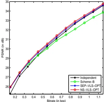
Simulation results are performed on five real stereo pairs down-loaded from1_{. In order to show the benefits of the proposed scheme,} we provide the results for the following decompositions carried out over three resolution levels. The first one consists of coding inde-pendently the left and right images using the 9/7 transform which was selected for the lossy mode of the JPEG2000 standard. This scheme will be designated by “Independent”. The second method, which will be denoted by “Scheme-B”, is the state-of the-art method where the reference and the residual images are encoded using also the 9/7 transform [7]. The third one corresponds to our previous joint stereo coding scheme based on a separable optimized VLS decomposition. Finally, we consider the proposed extension of this method to a non separable structure where a joint optimization approach is performed. The two latter methods will be designated respectively by “SEP-VLS-OPT” and “NS-VLS-OPT”. Fig. 2 dis-plays the scalability in quality of the reconstruction procedure by providing the variations of the average PSNR versus the average bitrate of the “houseof” stereo images. These plots show that the proposed method achieves an average gain of about 0.1-0.15 dB compared to our recent work “SEP-VLS-OPT”. The gain becomes more important (up to 0.65 dB) compared with the state-of-the art methods. Fig. 3 displays the reconstructed target image of the “aerial” stereo pairs for “Scheme-B” and “NS-VLS-OPT”. We no-tice that the coding of the residual image leads to blocking artefacts whereas our approach reduces significantly this problem. It is im-portant to emphasize here that the blocking artefacts appearing with the state-of-the-art method are not related to the wavelet codec and

1_{http://vasc.ri.cmu.edu/idb/html/stereo/index.html,}

http://vasc.ri.cmu.edu/idb/html/jisct/index.html

result mainly from the limitations of the generic scheme where a residual image is generated using a block-based approach. Finally, in order to measure the relative gain of the proposed method, we used the Bjontegaard metric [19]. The results are illustrated in Ta-ble 1 for low, middle and high bitrates corresponding respectively to the four bitrate points{0.15, 0.2, 0.25, 0.3}, {0.5, 0.55, 0.6, 0.65} and{1.25, 1.3, 1.35, 1.4} bpp. Table 1 gives the gain of the method “NS-VLS-OPT” compared with “Scheme-B”. Note that a bitrate saving with respect to the reference method corresponds to negative values. It can be observed that the proposed approach outperforms the classical one by about -20% and 0.2-1.4 dB in terms of bitrate saving and quality of reconstruction.

5. CONCLUSION

In this paper, we have exploited the flexibility offered by non separa-ble vector lifting schemes to perform a fully-optimized structure for joint coding of stereo images. Experiments have shown the benefits of the proposed method. In a future work, a new criterion defined simultaneously on the reference and the target images could be en-visaged. 0.2 0.3 0.4 0.5 0.6 0.7 0.8 0.9 1 1.1 26 27 28 29 30 31 32 33 34 35 Bitrate (in bpp) PSNR (in dB) Independent Scheme−B SEP−VLS−OPT NS−VLS−OPT

Fig. 2. PSNR (in dB) versus the bitrate (in bpp) after JPEG2000 progressive encoding of the stereo pair ’houseof’.

Table 1. The average PSNR differences and the bitrate saving at low, medium and high bitrates. The gain of “NS-VLS-OPT” w.r.t Scheme-B.

bitrate saving (in %) PSNR gain (in dB)

Images low middle high low middle high

houseof -1.07 -10.25 -11.31 0.04 0.46 0.87 pentagon -6.91 -21.68 -27.51 0.22 0.92 1.89 ball 1.91 -10.99 -18.29 -0.03 0.30 0.78 birch -15.17 -39.79 -23.70 0.81 1.13 2.12 aerial -0.45 -17.12 -19.44 0.02 0.75 1.43 average -4.34 -19.96 -20.05 0.21 0.71 1.41

(a) Original target image (b) PSNR=27.10 dB, SSIM=0.728 (c) PSNR=27.81 dB, SSIM=0.744 Fig. 3. Reconstructed target image of the “aerial” stereo pair at 0.3 bpp using (b) Scheme-B (c) NS-VLS-OPT.

6. REFERENCES

[1] I. Feldmann, W. Waizenegger, N. Atzpadin, and O. Schreer, “Real-time depth estimation for immersive 3D videoconfer-encing,” in 3DTV-Conference: The True Vision - Capture, Transmission and Display of 3D Video, Tampere, June 2010, pp. 1–4.

[2] M. G. Perkins, “Data compression of stereo pairs,” IEEE Transactions on Communications, vol. 40, no. 4, pp. 684–696, April 1992.

[3] D. Tzovaras, N. Grammalidis, and M.G. Strintzis, “Disparity field and depth map coding for multiview 3D image genera-tion,” Signal Processing: Image Communication, vol. 11, no. 3, pp. 205–230, January 1998.

[4] O. Woo and A. Ortega, “Stereo image compression based on disparity field segmentation,” in SPIE Conference on Visual Communications and Image Processing, San Jose, California, February 1997, vol. 3024, pp. 391–402.

[5] M. S. Moellenhoff and M. W. Maier, “Transform coding of stereo image residuals,” IEEE Transactions on Image Process-ing, vol. 7, no. 6, pp. 804–812, June 1998.

[6] J. Xu, Z. Xiong, and S. Li, “High performance wavelet-based stereo image coding,” in IEEE International Symposium on Circuits and Systems, May 2002, vol. 2, pp. 273–276. [7] N. V. Boulgouris and M. G. Strintzis, “A family of

wavelet-based stereo image coders,” IEEE Transactions on Circuits and Systems for Video Technology, vol. 12, no. 10, pp. 898– 903, October 2002.

[8] R. Darazi, A. Gouze, and B. Macq, “Adaptive lifting scheme-based method for joint coding 3D-stereo images with lumi-nance correction and optimized prediction,” in IEEE Interna-tional Conference on Acoustics, Speech and Signal Processing, Taipei, April 2009, pp. 917–920.

[9] A. Maalouf and M.-C. Larabi, “Bandelet-based stereo im-age coding,” in IEEE International Conference on Acoustics, Speech and Signal Processing, Dallas, Texas, United States, March 2010, pp. 698–701.

[10] E. Le Pennec and S. Mallat, “Sparse geometric image repre-sentations with bandelets,” IEEE Transactions on Image Pro-cessing, vol. 14, no. 4, pp. 423–438, April 2005.

[11] T. Frajka and K. Zeger, “Residual image coding for stereo image compression,” Optical Engineering, vol. 42, no. 1, pp. 182–189, January 2003.

[12] M. Kaaniche, A. Benazza-Benyahia, B. Pesquet-Popescu, and J.-C. Pesquet, “Vector lifting schemes for stereo image cod-ing,” IEEE Transactions on Image Processing, vol. 18, no. 11, pp. 2463–2475, November 2009.

[13] O. N. Gerek and A. E. C¸ etin, “Adaptive polyphase subband de-composition structures for image compression,” IEEE Trans-actions on Image Processing, vol. 9, no. 10, pp. 1649–1660, October 2000.

[14] V. Chappelier and C. Guillemot, “Oriented wavelet transform for image compression and denoising,” IEEE Transactions on Image Processing, vol. 15, no. 10, pp. 2892–2903, October 2006.

[15] M. Kaaniche, A. Benazza-Benyahia, B. Pesquet-Popescu, and J.-C. Pesquet, “Non separable lifting scheme with adaptive update step for still and stereo image coding,” Elsevier Signal Processing: Special issue on Advances in Multirate Filter Bank Structures and Multiscale Representations, vol. 91, no. 12, pp. 2767–2782, January 2011.

[16] M. Kaaniche, B. Pesquet-Popescu, A. Benazza-Benyahia, and J.-C. Pesquet, “Adaptive lifting scheme with sparse criteria for image coding,” EURASIP Journal on Advances in Signal Processing: Special Issue on New Image and Video Represen-tations Based on Sparsity, vol. 2012, 22 pages, January 2012. [17] J. Eckstein and D. P. Bertsekas, “On the Douglas-Rachford

splitting methods and the proximal point algorithm for max-imal monotone operators,” Mathematical Programming, vol. 55, pp. 293–318, 1992.

[18] P. L. Combettes and J.-C. Pesquet, “Proximal splitting meth-ods in signal processing,” in Fixed-Point Algorithms for Inverse Problems in Science and Engineering, H. H. Bauschke, R. Bu-rachik, P. L. Combettes, V. Elser, D. R. Luke, and H. Wolkow-icz, Eds. Springer-Verlag, New York, 2010.

[19] G. Bjontegaard, “Calculation of average PSNR differences be-tween RD curves,” Tech. Rep., ITU SG16 VCEG-M33, Austin, TX, USA, April 2001.