Point-scale evaluation of the Soil, Vegetation, and Snow (SVS) land surface model

(1)

Point-scale evaluation of the Soil, Vegetation, and Snow

(SVS) land surface model

Thèse

Gonzalo Americo Leonardini Quelca

Doctorat en génie des eaux

Philosophiæ doctor (Ph. D.)

(2)

Point-scale evaluation of the Soil, Vegetation, and

Snow (SVS) land surface model

Thèse

Gonzalo Leonardini

Sous la direction de:

François Anctil, directeur de recherche Vincent Fortin, codirecteur de recherche

(3)

Résumé

Le modèle de surface Soil, Vegetation, and Snow (SVS) a été récemment mis au point par Envi-ronnement et Changement climatique Canada (ECCC) à des fins opérationnelles de prévisions météorologique et hydrologique. L’objectif principal de cette étude est d’évaluer la capacité de SVS, en mode hors ligne à l’échelle de points de grille, à simuler différents processus par rapport aux observations in situ. L’étude est divisée en deux parties: (1) une évaluation des processus de surface terrestre se produisant dans des conditions sans neige, et (2) une évalua-tion des processus d’accumulaévalua-tion et de fonte de la neige. Dans la première partie, les flux d’énergie de surface et la teneur en eau ont été évalués sous des climats arides, méditerra-néens et tropicaux pour six sites sélectionnés du réseau FLUXNET ayant entre 4 et 12 ans de données. Dans une seconde partie, les principales caractéristiques de l’enneigement sont exa-minées pour dix sites bien instrumentés ayant entre 8 et 21 ans de données sous climats alpins, maritimes et taiga du réseau ESM-SnowMIP. Les résultats de la première partie montrent des simulations réalistes de SVS du flux de chaleur latente (NSE = 0.58 en moyenne), du flux de chaleur sensible (NSE = 0.70 en moyenne) et du rayonnement net (NSE = 0.97 en moyenne). Le flux de chaleur dans sol est raisonnablement bien simulé pour les sites arides et un site méditerranéen, et simulé sans succès pour les sites tropicaux. Pour sa part, la teneur en eau de surface a été raisonnablement bien simulée aux sites arides (NSE = 0.30 en moyenne) et méditerranéens (NSE = 0.42 en moyenne) et mal simulée aux sites tropicaux (NSE = −16.05 en moyenne). Les performances du SVS étaient comparables aux simulations du Canadian Land surface Scheme (CLASS) non seulement pour les flux d’énergie et le teneur en eau, mais aussi pour des processus plus spécifiques tels que l’évapotranspiration et le bilan en eau. Les résultats de la deuxième partie montrent que SVS est capable de reproduire de manière réa-liste les principales caractéristiques de l’enneigement de ces sites. Sur la base des résultats, une distinction claire peut être faite entre les simulations aux sites ouverts et forestiers. SVS simule adéquatement l’équivalent en eau de la neige, la densité et la hauteur de la neige des sites ouverts (NSE = 0.64, 0.75 et 0.59, respectivement), mais présente des performances plus faibles aux sites forestiers (NSE = −0.40, 0.15 et 0.56, respectivement), ce qui est principale-ment attribué aux limites du module de tasseprincipale-ment et à l’absence d’un module d’interception de la neige. Les évaluations effectuées au début, au milieu et à la fin de l’hiver ont révélé une tendance à la baisse de la capacité de SVS à simuler SWE, la densité et l’épaisseur de la neige

(4)

à la fin de l’hiver. Pour les sites ouverts, les températures de la neige en surface sont bien représentées (RMSE = 3.00 ◦C en moyenne), mais ont montré un biais négatif (PBias = −1.6 % en moyenne), qui était dû à une mauvaise représentation du bilan énergétique de surface sous conditions stables la nuit. L’albédo a montré une représentation raisonnable (RMSE = 0.07 en moyenne), mais une tendance à surestimer les valeurs de fin d’hiver (biais = 0,04 sur la fin de l’hiver), en raison de la diminution progressive pendant les longues périodes de fonte. Enfin, un test de sensibilité a conduit à des suggestions aux développeurs du modèles. Les tests de sensibilité du processus de fonte de la neige suggèrent l’utilisation de la température de surface de la neige au lieu de la température moyenne lors du calcul. Cela permettrait d’améliorer les simulations SWE, à l’exception de deux sites ouverts et d’un site forestier. Les tests de sensibilité à la partition des précipitations permettent d’identifier une transition linéaire de la température de l’air entre 0 et 1 ◦C comme le meilleur choix en l’absence de partitions observées ou plus sophistiquées.

(5)

Abstract

The Soil, Vegetation, and Snow (SVS) land surface model has been recently developed at Environment and Climate Change Canada (ECCC) for operational numerical weather pre-diction (NWP) and hydrological forecasting. The main goal of this study is to evaluate the ability of SVS, in offline point-scale mode, to simulate different processes when compared to in-situ observations. The study is divided in two parts: (1) an evaluation of land-surface processes occuring on snow-free conditions, and (2) and evaluation of the snow accumulation and melting processes. In the first part, surface heat fluxes and soil moisture were evaluated under arid, mediterranean, and tropical climates at six selected sites of the FLUXNET net-work having between 4 and 12 years of data. In the second part, the main characteristics of the snow cover are examined at ten well-instrumented sites having between 8 and 21 years under alpine, maritime and taiga climates from ESM-SnowMIP network. Results of the first part show SVS’s realistic simulations of latent heat flux (NSE = 0.58 on average), sensible heat flux (NSE = 0.70 on average), and net radiation (NSE = 0.97 on average). Soil heat flux is reasonably well simulated for the arid sites and one mediterranean site, and poorly simulated for the tropical sites. On the other hand, surface soil moisture was reasonably well simulated at the arid (NSE = 0.30 on average) and mediterranean sites (NSE = 0.42 on aver-age) and poorly simulated at the tropical sites (NSE = −16.05 on averaver-age). SVS performance was comparable to simulations of the Canadian Land Surface Scheme (CLASS) not only for energy fluxes and soil moisture, but more specific processes such as evapotranspiration and water balance. Results of the second part show that SVS is able to realistically reproduce the main characteristics of the snow cover at these sites. Based on the results, a clear dis-tinction between simulations at open and forest sites can be made. SVS is able to simulate well snow water equivalent, density and snow depth at open sites (NSE = 0.64, 0.75 and 0.59, respectively), but exhibits lower performances over forest sites (NSE = −0.40, 0.15 and 0.56, respectively), which is attributed mainly to the limitations of the compaction scheme and the absence of a snow interception scheme. Evaluations over early, mid and end winter periods revealed a tendency to decrease SVS’s ability to simulate SWE, density and snow depth during end winter. At open sites, SVS’ snow surface temperatures are well represented (RMSE = 3.00◦C on average), but exhibited a cold bias (PBias = −1.6% on average), which was due to a poor representation of the surface energy balance under stable conditions at nighttime.

(6)

Albedo showed a reasonable representation (RMSE = 0.07 on average), but a tendency to overestimate end winter albedo (bias = 0.04 over end winter), due to the slow decreasing rate during long melting periods. Finally, sensitivity tests to the snow melting process suggest the use of surface snow temperature instead of the average temperature when computing the melting rate. This would provide the improvement of the SWE simulations, with exception of two open and one forest sites. Sensitivity tests to partition of precipitation allows to identify a linear transition of air temperature between 0 and 1◦C as the best choice in the absence of observed or more sophisticated partitions.

(7)

List of Tables

2.1 Main characteristics of the study sites. . . 13 2.2 Summary of SVS and CLASS main physical processes. . . 16 2.3 Parameters for SVS and CLASS models at each FLUXNET site used in this

study. . . 17 2.4 Main characteristics of the study sites. . . 18 2.5 SVS parameters used in the experiments. . . 21 3.1 Scores for the latent heat flux (LE), sensible heat flux (H), net radiation (Rn),

and soil heat flux (G) for a 30-min time step. The bold numbers correspond to

the best score between both models. . . 24 3.2 Scores between observations and simulations (SVS and CLASS) of the surface

water content for all the study sites. The scores were obtained for 30-min

sampling intervals. The bold numbers correspond to the best score. . . 33 4.1 Scores for modeled SWE, snow density, and depth against manual observations

(10)

List of Figures

1.1 Diagram of the land surface tiling approach implemented into SVS model in the absence of snow (a) and in the presence of snow (b). The fraction of each

tiling component is indicated in parenthesis. . . 8 1.2 Schematic diagram of SVS energy flux terms. Arrows represent input and

out-put of energy for each tile component. Red/blue arrows correspond to the

energy gained/lost by tiling component. . . 9 1.3 Schematic diagram of SVS water-associated terms. Arrows represent input and

output of energy for each tile component. Red/blue arrows correspond to the

energy gained/lost by tiling component. . . 10 2.1 Location of the FLUXNET study sites. Alice Springs (AU-ASM) in Australia;

Walnut Gulch Kendall Grasslands (US-Wkg) and Tonzi Ranch (US-Ton) in the United States; Arca di Noe-Le Prigionette (IT-Noe) in Italy; Pasoh Forest

Reserve (MY-PSO) in Malaysia; Guyaflux (GF-Guy) in French Guiana. . . 13 2.2 Mean monthly air temperature and precipitation for the studied periods, sorted

according to climate type. Arid sites: (a) AU-ASM, (b) US-Wkg; mediterranean

sites: (c) US-Ton, (d) IT-Noe; tropical sites: (e) MY-PSO, (f) GF-Guy. . . 14 2.3 Monthly mean (a) rainfall, (b) snowfall, (c) air temperature, (d) wind speed, (e)

solar radiation, (f) infrared radiation, (g) specific humidity, and (h) atmospheric

pressure at the ESM-SnowMIP sites. . . 20 3.1 Mean annual cycles of latent heat flux (LE), sensible heat flux (H), net

radi-ation (R_n), and soil heat flux (G): observations (black line), SVS simulations (blue line), CLASS simulations (red line). Filtered 30-min data for observations and simulations were used to compute the mean annual cycles. Note that the

y-axis for G differs from the rest of the graphs. . . 23 3.2 Mean annual cycles of evapotranspiration (ET ), soil evaporation (Es),

transpi-ration (T s), and wet canopy evapotranspi-ration (Ec) for observations (black line) and

SVS (blue line) and CLASS simulations (red line). . . 26 3.3 Partitioning of the precipitation into the different water balance terms, namely

evapotranspiration, ET (green); overland flow, R_surf (blue); base flow, R_base

(yellow); and storage in the soil column, ∆S (red) . . . 28 3.4 Precipitation and soil water content at 30-min time steps for the AU-ASM arid

site: (a) precipitation; (b) soil water content at the surface layer (0 - 10 cm) for observations (black line), SVS simulations (blue line) and CLASS simulations (red line); simulated soil water content profile for the (c) SVS and (d) CLASS

(11)

3.5 Precipitation and soil water content at 30-min time steps for the US-Ton mediterranean site: (a) precipitation; (b) soil water content at the surface layer (0 -10 cm) for observations (black line), SVS simulations (blue line) and CLASS simulations (red line); simulated soil water content profile for (c) SVS and (d)

CLASS models. . . 31 3.6 Precipitation and soil water content at 30-min sampling intervals for the

MY-PSO tropical site: (a) precipitation; (b) soil water content at the surface layer (0 - 10 cm) for observations (black line), SVS simulations (blue line) and CLASS simulations (red line); simulated soil water content profile for (c) SVS and (d)

CLASS models. . . 32 4.1 Diagram of the SVS performances for SWE, snow density (DEN) and depth

(SD) for the periods of December-January (DJ), February-March (FM) and April-May (AM) at open (text in orange) and subcanopy (text in green) sites.

(a) NSE, (b) PBias and (c) r scores. . . 37 4.2 Comparison between simulated and observed (A) SWE, (B) snow density and

(C) depth for winters 2006/07 and 2007/08 at Col de Porte (CDP). Results from SVS (blue line), Crocus (red line), automatic observations (black line)

and manual observations (black squared dots) are reported. . . 38 4.3 Categorical frequency distribution of ∆SD for observations (black), SVS (blue),

and Crocus (red) at the CDP site, for the period 1994-2014. . . 40 4.4 Cumulated positive ∆SD for SVS (blue), Crocus (red) and observations (black),

by categories at all sites. . . 41 4.5 Cumulated negative ∆SD for SVS (blue), Crocus (red) and observations (black)

by categories at five sites for all days (solid lines, left panel) and MSD (dashed

lines, right panel). . . 42 4.6 Quantile - quantile (Q-Q)plots of observed and simulated daily snow surface

temperature (◦C) at CDP, SWA, SNB, WFJ, and SAP for the SVS (a-e) and Crocus (f-j) models for December and January (DJ) in red, February and March

(FM) in green, and April and May (AM) in blue. RMSE and bias are also given. 43 4.7 Hourly air temperature (a) and snow surface temperature (b) for SVS in blue,

Crocus in red, and the observations in black at CDP site for February 2008. . . 44 4.8 Same as in Figure 4.5, but for April 2008. . . 45 4.9 Quantile - quantile (Q-Q) plots of observed and simulated daily albedo at CDP,

SWA, SNB, WFJ, and SAP for SVS (a-e) and Crocus (f-j) for December-January (DJ) in red, February-March (FM) in green, and April-May (AM) in blue.

RMSE and bias are also given. . . 46 4.10 Daily average of snow surface albedo simulated by SVS and Crocus for the

2007/08 winter at CDP site. Observations are represented by circles. . . 46 4.11 Sensitivity experiments on SWE at all sites: Simulations with the reference

configuration (Ref ), with no melt associated with rainfall (NoMeltRain), us-ing the snow surface temperature for the meltus-ing calculation (Melt ), with 0◦C threshold partition of precipitation (c1 ), with a linear transition at 0<Tair<2◦C (c2 ), and a polynomial transition (Auer Jr, 1974) at 0<Tair<6◦C (c3 ). The

(12)

C.1 Precipitation and soil water content at 30-min time steps for the US-Wkg arid site: (a) precipitation; (b) soil water content at the surface layer (0 - 10 cm) for observations (black line), SVS simulations (blue line) and CLASS simulations (red line); simulated soil water content profile for the (c) SVS and (d) CLASS

models. . . 58 C.2 Precipitation and soil water content at 30-min time steps for the IT-Noe

Mediterranean site: (a) precipitation; (b) soil water content at the surface layer (0 -10 cm) for observations (black line), SVS simulations (blue line) and CLASS simulations (red line); simulated soil water content profile for the (c) SVS and

(d) CLASS models.. . . 59 C.3 Precipitation and soil water content at 30-min time steps for the GF-Guy

trop-ical site: (a) precipitation; (b) soil water content at the surface layer (0 - 10 cm) for observations (black line), SVS simulations (blue line) and CLASS sim-ulations (red line); simulated soil water content profile for the (c) SVS and (d)

CLASS models. . . 60 C.4 Scatter plots of observed and simulated snow depth (SD) for SVS and Crocus

for all the study sites. RMSE and bias are also given. . . 61 C.5 Scatter plots of observed and simulated snow water equivalent (SWE) for SVS

and Crocus for all the study sites. RMSE and bias are also given. . . 62 C.6 Scatter plots of observed and simulated snow density for SVS and Crocus for

(13)

To Teodocia, Elías, Carlos, Elisa and Susy.

(14)

Acknowledgments

First of all, it is important for me to thank my thesis supervisors François Anctil and Vin-cent Fortin. François for his confidence and his patience in my work. He always brought enlightening ideas at the several times I was stuck, and he always knows the right answer to all my questions. Thank you François. Vincent Fortin was supporting my work always at the right moment and in the right way. Thank you Vincent. This work could not be possible without the collaboration of Vincent Fortin’s team: Vincent Vionnet, Maria Abrahamowicz and Étienne Gaborit from Environment and Climate Change Canada. I think they are not aware of how rich, from a work-experience perspective, was for me every discussion, even when the decision was to change the perspective of some result. Finally, I thank Daniel Nadeau for his enthusiasm and meticulous support during this thesis. You are the dream team of any doctoral student, for sure!

I must thank all the colleagues who participated directly or indirectly on my work: Philippe Richard, Achut Parajuli, Bram Hadiwijaya, Georg Lackner, Antoine Thiboult, Emixi Valdez, Marco Alves, Alicia Talbot-Lanciault, Carine Poncelet, Yamazaki-sensei, Julia Ledergerber, Lida Sánchez Sanchez, Christian Arias, Darwin Brochero. You all contributed in different ways to this thesis, but each of those ways was absolutely essential. Thank you very much. Special thanks to the members of the jury of my early doctoral examinations: Audrey Maheu, Peter Vanrolleghem, Brian Morse and Daniel Nadeau. Your insights were helpful throughout the rest of my thesis work.

This doctorate allowed me to focus on research without worrying about anything else. I ac-knowledge the organizations and institutions that provided me any type of financial support: the Natural Sciences and Engineering Research Council of Canada (NSERC), Hydro-Québec, the Ouranos consortium on regional climatology and adaptation to climate change, Environ-ment and Climate Change Canada, and the Quebec Water Research Center (CentrEau). Outside of the University, I must thank family and friends for their kind support and patience during all this years. Your encouragement was essential to maintain the level of motivation necessary for my doctoral studies. I particularly express my gratitude to my parents Teodocia and Elías, my sister Elisa, my brother Carlos, also to my sister-in-law Susy, my nieces Rafaela

(15)

and Diana, my grandparents Carlos Quelca, and Carlos Leonardini. Thanks to Jaime Siles y Hortensia Siles for your kindness and hospitality and all the warm pieces of advice. Finally thanks to Chantal Giroux, Sebastian Gutierrez, Karen Losantos and Juan Kutipa for all the selfless and permanent support.

(16)

Foreword

This thesis is based on two scientific articles, one published and one in preparation. The first article can be found as:

Leonardini, G., Anctil, F., Abrahamowicz, M., Gaborit, É., Vionnet, V., Nadeau, D. F., & Fortin, V. (2020). Evaluation of the Soil, Vegetation, and Snow (SVS) Land Surface Model for the Simulation of Surface Energy Fluxes and Soil Moisture under Snow-Free Conditions. Atmosphere, 11(3), 278; https://doi.org/10.3390/atmos11030278.

This article was submitted on February 8, 2020, accepted by the editor on March 9, 2020, and published on March 12, 2020. The version in this thesis is taken directly from the published manuscript. For this article, I was the lead author: I analyzed the data to create the results of the article, I wrote the vast majority of the text and applied the corrections suggested by the reviewers. François Anctil supervised the scientific work and revised the manuscript in depth, Vincent Fortin (from Environment and Climate Change Canada, ECCC) co-supervised the scientific work and revised the manuscript, Maria Abrahamowicz (ECCC) helped to improve the model code and revised the manuscript, Étienne Gaborit and Vincent Vionnet (ECCC) assisted in setting up the SVS model in offline and point-scale configuration and reviewed the manuscript. Daniel Nadeau revised the manuscript in detail. This research was founded by the Natural Sciences and Engineering Research Council of Canada (NSERC), Hydro-Québec and the Ouranos consortium on regional climatology and adaptation to climate change, and the Ministère de l’Environnement et de la Lutte contre les changements climatiques through NSERC project RDC-477125-14 entitled "Modélisation hydrologique avec bilan énergétique (ÉVAP)"

By the time this thesis is presented, a second article has been submitted to the Journal of Hydrometeorology (JHM):

Leonardini, G., Anctil, F., Vionnet, V., Abrahamowicz, M., Nadeau, D. F., & Fortin, V. (in prep.). Evaluation of the snow cover in the Soil, Vegetation, and Snow (SVS) Land Surface Model.

(17)

François Anctil and Vincent Fortin supervised the scientific work and revised the manuscript. Vincent Vionnet and Maria Abrahamowicz assisted improving the SVS code, giving scien-tific advice and revising the manuscript. Daniel Nadeau revised the manuscript in detail. This study was founded by Natural Sciences and Engineering Research Council of Canada (NSERC), Hydro-Québec and the Ouranos consortium on regional climatology and adapta-tion to climate change, and the scientific contribuadapta-tion of Environment and Climate Change Canada and the Ministère de l’Environnement et de la Lutte contre les changements clima-tiques through NSERC project RDC-477125-14 entitled “Modélisation hydrologique avec bilan énergétique (ÉVAP)”. I also acknowledge ECCC financial support through Grant & Contri-bution project GCXE20M014 entitled “Évaluation et amélioration du schéma de surface SVS (Soil, Vegetation and Snow)”. I also would like to thank to Matthieu Lafaysse and his team from the Centre National de Recherches Météorologiques (CNRM) for providing the outputs of CROCUS model. This work used the meteorological and evaluation ESM-SnowMIP datasets:.

(18)

Introduction

About 29% of the Earth’s surface is covered by land and represents an essential component of the Earth’s climate system. The land surface incorporates the components of soil, vegeta-tion, snow, etc. Land surface processes refer to various biogeophysical, biogeochemical and hydrologic processes occurring within and over these components and interacting with the at-mospheric processes. Land surface models (LSMs) are mathematical descriptions of the land surface processes, with particular attention to momentum, energy, and mass flux exchanges with the overlaying atmosphere. In the frame of Earth system modelling (ESM), LSMs are designed to provide the atmospheric model with lower boundary conditions over global land areas, describing the interactions of the land surface with the atmosphere. To accomplish their objectives, LSMs maintain a number of state variables that are of interest to other domain such as hydrology, ,icrometeorology, agroclimatology, etc. Soil water content and temperature, snowpack characteristics, and lateral flows are typical examples that are at the centre of the present thesis.

Surface energy balance

There are several fundamental equations that describe the role of land surface processes in the atmosphere. The two main equations are the energy and surface water balances. According to Pitman(2003), the energy balance, applied to a surface, is defined as follows:

Rn= H + LE + G, (1)

where Rn is the net radiation, H and LE are the sensible and latent heat fluxes respectively,

and G is the soil heat flux. Rn includes the net shortwave and net longwave radiations fluxes.

The partition of R_n into H and LE, represented by Equation 1, is mainly controlled by the land surface hydrometeorological conditions such as plant transpiration, the soil surface temperature.

(19)

Surface water balance

Precipitation that falls to the Earth’s surface is either intercepted by the vegetation or reaches the soil surface directly. Precipitation that is intercepted either evaporates or drips to the surface. All the water that reaches the surface, either infiltrates into the soil or runs across the soil surface (surface runoff). Water that infiltrates may evaporate from the soil surface, drain through the soil, or be taken up by roots and transpired. While the water is in the soil, it is known as soil moisture.

The water balance of a land surface column between the incoming and outgoing fluxes of water is defined as:

P = ET + Rsurf + Rbase+ ∆S, (2)

where P is precipitation, ET is evapotranspiration, R_surf is the overland flow (possibly in-cluding subsurface lateral flow), R_baseis the drainage (vertical flow from the bottom of the soil column), and ∆S is the variation in the water stored in the soil, vegetation and snow layers. Note that ET is linked to the surface energy balance by the latent heat flux term, LE = λET , where λ is the latent heat of vaporization.

On the land surface modelling evolution

LSMs for use in weather and climate modeling have been the subject of intense development over the last three decades (Pitman, 2003; van den Hurk et al., 2011). They consolidate knowledge acquired from micrometeorology, soil science, as well as field and laboratory research on plant physiology.

LSMs typically are classified into three generations (Pitman,2003;Sellers et al.,1997). The first-generation is well represented by the LSM implemented by Manabe (1969). This LSM uses a simple energy balance equation, ignoring heat conduction into the soil. It relies on a constant soil depth and water-holding capacity, where evaporation is limited by a soil water content threshold. If the soil moisture surpass a prescribed limit, then further precipitation generate runoff. Such parameterization is commonly named "Manabe bucket model". In first-generation models, the transfer of sensible and latent heat is based on simple aerodynamic bulk transfer formulations, using uniform and prescribed surface parameters such as water holding capacity, albedo, and roughness length. These models do not account for ecological processes (e.g., transpiration of plants through stomata) or more detailed hydrological processes (e.g., infiltration and capillary upward flow through soil micropores). Despite their simplifications, they represent a key step to describe land surface processes in ESMs and their simulated soil moisture and evapotranspiration time series are comparable to more complex models at longer timescales (Henderson-Sellers et al.,1996).

(20)

Second-generation schemes were influenced by the work of Deardorff (1978) who developed a method for simulating soil temperature and moisture in two layers and vegetation as a single bulk layer. Deardorff’s soil model was based on the "force-restore" soil schemes of Bhum-ralkar (1975) andBlackadar (1976). Second generation LSMs explicitly represents vegetation effects and include more complex soil hydrology in the calculation of surface energy and wa-ter balances (Dickinson,1984;Sellers et al.,1986;Deardorff,1978). During this development period, various second-generation models were proposed putting emphasis on various specific processes (e.g. Desborough and Pitman,1998;Thompson and Pollard, 1995;Verseghy et al., 1993;Xue et al.,1991). These models vary in detail but share many features. They usually exploit a number of soil layers, a single canopy layer, and a bulk snow layer. Micrometeoro-logical, hydroMicrometeoro-logical, and ecological processes are more explicitly represented in these models. Instead of the fixed surface albedo such as for the first-generation models, more explicit ra-diation transfer through the vegetation canopy differentiating visible and near-infrared and beam and diffusive lights are taken into account. Turbulent transfer of heat from multiple surface sources, for example canopy leaves and the ground surface are considered, and the under-canopy and leaf boundary layer turbulences are parameterized based on atmospheric boundary layer similarity theories. Transpiration of plants through stomata are considered using the Jarvis-type stomatal conductance scheme (Jarvis,1976), a simple empirical formu-lation that is a function of light (PAR; photosynthetically active radiation), water (leaf water potential), and environmental conditions (air temperature and humidity). Whether the soil moisture Richards equation is solved or not, vertical gravity and capillary flows of water are taken into account. Runoff is parameterized as various functions of soil water storage or excess above infiltration, neglecting topographic effects. Accumulation and ablation of snow on the ground are represented with a bulk layer of snow, neglecting internal processes within the snowpack.

The third-generation models are mainly characterized by their capability in simulating carbon uptake by plants and vegetation dynamics (Pitman,2003;Sellers et al.,1997). Other aspects of the model are substantially improved at the same time. Some models even incorporate treatments of nutrient dynamics and biogeography, so that vegetation systems can change location in response to climate shifts. Collatz et al. (1991) andSellers et al. (1992) began to integrate stomatal conductance and photosynthesis into LSMs, based on the work ofFarquhar et al. (1980). A semiempirical model of leaf conductance was also proposed (Collatz et al., 1992), based on the understandings of the limitations on carbon assimilation by leaf and maximum use of water by plants (Ball,1988).

In the course of the same time period, LSMs were largely improved in other aspects in respect of representations of hydrological processes in ESMs. LSMs started to account for subgrid variability in a more explicit way, for example, a "tile" approach to represent vegetation heterogeneity (Koster and Suarez,1992;Avissar and Pielke,1989) and a statistical approach to

(21)

represent subgrid distribution of soil moisture and runoff generation (Entekhabi and Eagleson, 1989), spatial variability of infiltration (Liang et al.,1994), topographic control on subgrid soil moisture distribution and runoff generation (Niu et al., 2005; Famiglietti and Wood, 1994), and subgrid snow distribution (Niu et al., 2007; Liston, 2004). LSMs started to include more physically based, multilayer snow submodels to accommodate more internal processes by parameterizing growth of grain size and liquid water retention and percolation within snowpack (Yang and Niu,2003;Dai et al.,2003;Jin et al.,1999). Ice content within soil was explicitly resolved as a new prognostic variable, and its impacts on runoff and infiltration were investigated (Niu and Yang, 2006; Koren et al., 1999; Pitman et al., 1999). Most recently, groundwater processes were implemented in LSMs (Niu et al.,2007;Fan et al.,2007;Yeh and Eltahir, 2005; Maxwell and Miller, 2005; Liang et al., 2003), and LSMs have entered into a new era involving multiple disciplinary sciences.

Point-scale model validation

The quality of a LSM model can be assessed by comparing its output with observed values. A set of global and regional scale datasets that can be used to validate results from GCM climate runs or to monitor the performance of NWP assimilation/forecast systems is often used (e.g. Jaeger,1983;Wallis et al.,1991). In this type of validation, it is not always obvious how to link errors in the variables to deficiencies in one specific parametrization scheme. For instance, feedbacks between model processes can be responsible for model deficiencies in a variable such as precipitation (Arpe, 1991). Some of the datasets are estimated; for instance, latent-heat fluxes and the other components of the surface energy balance are estimated based on the extent of empirical formulas and energy-conservation principles (GCIP, 1995-2000). Although making the dataset self-consistent in energetic terms, these methods cast some doubt on their validity for verifying model results.

Stand alone (LSM uncoupled of the atmospheric model), and point-scale simulations require a continuous time series of meteorological forcing. The advantages are: i) it allows for the mitigation of biases in the atmospheric forcing fields; ii) it allows the simulations to run more quickly than in coupled mode and it facilitates the examination on model sensitivities; iii) it permits to examine in detail multiple sites and long time series. On the other hand, because of the absence of feedback from the boundary layer, model drifts are perhaps exaggerated in this validation exercise (Jacobs and De Bruin,1992). Nevertheless, point-scale validation remains the only form of validation giving a clear message about the identification of shortcomings in the simulation that are purely related to the formulation of the land surface scheme.

The model validation at point-scale is based on the quality of the in-situ micrometeorological and hydrometeorological observations. This quality is associated with the technical progress in the instrumentation (Foken, 2008) and the efforts to group individual observations into

(22)

networks where the procedures and data pipelines are standardized. In recent years, many organizations or communities have established high-quality land surface observation systems (Lautenbacher, 2006; Scholes et al., 2008). For example, a regional and global network of micrometeorological tower sites (FLUXNET) operated on a long-term and continuous basis to measure the exchanges of carbon dioxide, water vapor, and energy between terrestrial ecosystems and the atmosphere by using Eddy covariance method for different landscapes. Another example in the context of snow concern the in situ observations of the Earth System Model Snow Intercomparison Project (ESM-SnowMIP, Krinner et al., 2018; Ménard et al., 2019). This data set include meteorological, snow, and soil observations from 10 reference sites covering a wide range of climates. FLUXNET and ESM-SnowMIP will be discussed later, but we mention here the capital importance of measurement campaigns and networks on which this entire study is based.

Problem statement

Environment and Climate Change Canada (ECCC) currently uses a modified version of the Interaction between Soil, Biosphere, and Atmosphere (ISBA) LSM to produce operational weather forecasts (Bélair et al.,2003b,a;Bélair et al.,2009). To address particular limitations with their operational version of ISBA (Bélair et al.,2003b,a), ECCC developed the Soil, Veg-etation, and Snow (SVS) LSM. As documented byAlavi et al.(2016) andHusain et al.(2016), SVS can be classified as a second-generation LSM that introduces the following improvements over ISBA: a new tiling approach, an improved parameterization of the vegetation thermal coefficient, the inclusion (as an option) of photosynthesis processes, a new formulation of land surface albedo and emissivity, a root density function that depends on the vegetation type, an update of the snow melt process, and multilayer vertical water transport in the soil.

SVS has mostly been evaluated on the North-American domain (Alavi et al., 2016; Husain et al.,2016). In general, it performs better than its predecessor over the warm season. It has been successfully implemented as part of the GEM-Hydro hydrological modelling platform to produce runoff simulations over Lake Ontario basin (Gaborit et al.,2017) and hindcasts of the major June 2013 flood in Alberta (Canada) (Vionnet et al.,2020). More recently, point-scale evaluations showed competitive results when contrasted to observations and more complex models over Mediterranean and temperate climates in the United States (Maheu et al.,2018). As part of of the work leading up to this thesis,Leonardini et al.(2020) conducted an evaluation of the energy fluxes and the soil moisture under arid, Mediterranean and tropical climates. While previous studies have assessed SVS’s general performance and contrasted it with ISBA, there has been no detailed evaluation of SVS snow model.

From a more practical perspective, ECCC intends to make SVS LSM operational for weather forecasting from 2021 (Vincent Fortin, personal communication), and the NWP models are

(23)

particularly sensitive to the energy fluxes and to the albedo estimated by SVS. Thus, a detailed examination of different process of SVS is necessary before its operational implementation.

Objectives

The purpose of this study is to evaluate the integrity of SVS through diverse climatic conditions in a multi-year and multi-site context. Two specific objectives are identified: (1) to evaluate the ability of SVS to simulate surface energy fluxes and soil moisture in snow-free conditions for various climate and biome types; (2) to assess to what degree SVS snow cover component is able to adequately represent the main characteristics of snowpacks.

(24)

Chapter 1

The Soil, Vegetation, and Snow (SVS)

model

Environment and Climate Change Canada (ECCC) currently uses a modified version of the Interaction between Soil, Biosphere, and Atmosphere (ISBA) LSM to produce operational weather forecasts Bélair et al.(2003b,a);Bélair et al.(2009). ISBA provides surface fluxes of momentum, water, and energy to the Global Environmental Multiscale (GEM) atmospheric model. To address particular limitations with their operational version of ISBA Bélair et al. (2003b,a), ECCC developed the Soil, Vegetation, and Snow (SVS) LSM. As documented by Alavi et al. (2016) and Husain et al. (2016), SVS introduces the following improvements compared to ISBA: a new tiling approach, an improved parameterization of the vegetation thermal coefficient, the inclusion (as an option) of photosynthesis processes, a new formulation of land surface albedo and emissivity, a root density function that depends on the vegetation type, an update of the snow melt process, and multilayer vertical water transport in the soil.

1.1 Tiling approach and vertical layering

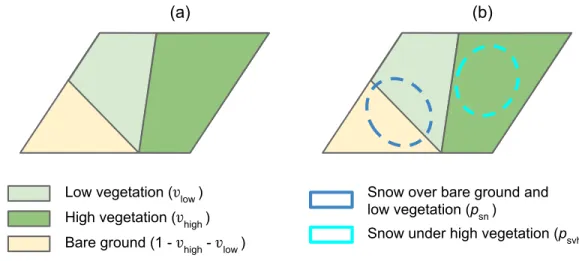
The tiling approach in SVS has been substantially modified from ISBA model as shown in Figure 1.1. Instead of a single energy budget for the entire land surface fraction of a model grid cell, SVS incorporates separate energy budgets for the individual land surface components within each grid cell. The land surface tiling is done in two steps. First, the land tile is divided into bare ground, low vegetation, and high vegetation fractions, adding up to a hundred percent. These three land cover types are then further split into a snow or no-snow areas, with corresponding fractions. The high and low vegetation fractions, v_high and v_low, are provided as input to SVS. If a particular vegetation type is deemed to be high enough not to be covered by snow (i.e., forests), it is considered to be “high”, otherwise it is specified as “low”. The remainder of the land, i.e., (1 − v_low− v_high) , is considered as bare ground. Based on the previous approach, the current implementation of SVS includes separate energy budgets for

(25)

(1) bare ground, (2) vegetation (high and low are aggregated), (3) snow covering bare ground and low vegetation, and (4) snow covering the ground under high vegetation.

The model considers a single-layer approach for the vegetation canopy, a one-layer snowpack and a one layer of soil for computing the energy budgets and temperatures. However, a user-defined number of soil layers and its respective depths, is set to compute soil moisture.

Bare ground (1 - v_high - v_low) Low vegetation (v_low) High vegetation (v_high)

Snow over bare ground and low vegetation (p_sn)

Snow under high vegetation (p_svh)

(a) (b)

Figure 1.1: Diagram of the land surface tiling approach implemented into SVS model in the absence of snow (a) and in the presence of snow (b). The fraction of each tiling component is indicated in parenthesis.

1.2 Energy fluxes

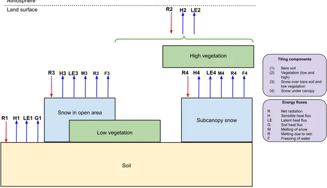
As illustrated in Figure 1.2, the energy budgets for the tiles (1)-(4) are obtained using the force-restore approach (Bélair et al.,2003a;Douville et al.,1995;Bhumralkar,1975). The net radiation for each tile component is estimated taking into account the balance between the direct and diffuse solar and infrared radiations at the surface, and the reflected and re-emitted radiations from the surface. The albedo and emissivity for bare ground are provided as an input to the model, but in the case of bare ground, they can also be computed based on the sand and clay fraction in the soil, as well as the soil wetness (Husain et al.,2016). The sensible and latent heat fluxes for each tile component are modeled using the bulk aerodynamic approach (Husain et al.,2016). In the presence of different vegetation types, in a single grid cell, a single energy budget is calculated using mean vegetation parameters (such as albedo and emissivity) based on a weighted mean of the parameters of each individual type of vegetation and their respective fractional coverage. The vapor flux from vegetation, required to compute the latent heat flux, is computed as a function of the moisture content of the interception reservoir given by Deardorff (1978), and the aerodynamical surface resistance for the vegetation. The

(26)

calculation of the aerodynamical surface resistance is obtained either from the photosynthesis approach (Husain et al.,2016;Collatz et al.,1992,1991;Farquhar et al.,1980) or the Jarvis-type approach (Husain et al.,2016;Noilhan and Planton,1989;Jarvis,1976) as used in ISBA. The soil heat flux was computed as the residual of the net radiation and the sensible and latent heat fluxes. In presence of snow, the fluxes of melting of snow, melting due to rainfall, and freezing of snow are accounted for the energy balance.

R1 R3 R4 R2 H1 LE1 H3 LE3 H4 LE4 H2 LE2 Atmosphere Land surface High vegetation Low vegetation Soil Subcanopy snow Snow in open area

M3 R3 M4 R4

Tiling components

(1) Bare soil

(2) Vegetation (low and

high)

(3) Snow over bare soil and

low vegetation

(4) Snow under canopy

Energy fluxes

R Net radiation

H Sensible heat flux

LE Latent heat flux

G Soil heat flux

M Melting of snow

R Melting due to rain

F Freezing of water

F3 F4

G1

Figure 1.2: Schematic diagram of SVS energy flux terms. Arrows represent input and output of energy for each tile component. Red/blue arrows correspond to the energy gained/lost by tiling component.

1.3 Soil

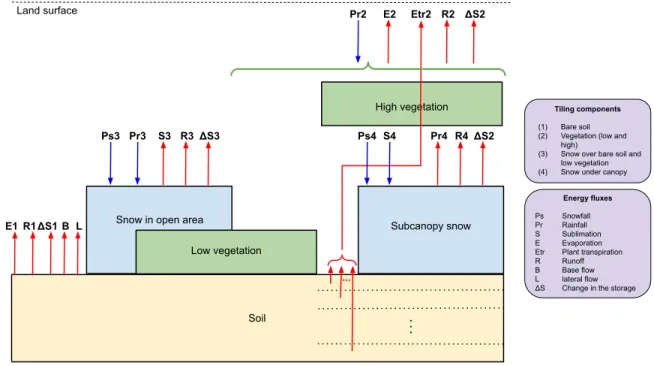
The evolution of volumetric soil moisture in different soil layers is calculated using the diffusion equation (Alavi et al., 2016). Liquid water flow is calculated using the Darcian equation for one-dimensional fluid flow along with the hydraulic conductivity and soil water suction followingClapp and Hornberger(1978). The saturated volumetric water content, wilting point volumetric water content and volumetric water content at field capacity are calculated based on the percentage of sand and clay contents in the soil according to Boone et al.(1999) and Soulis et al. (2011). The saturated hydraulic conductivity and saturated soil water potential are calculated from the percentage of sand as specified byBrooks and Corey(1966). The lateral flow in the downhill direction is estimated through a parameterization of Richard’s equation, which estimates lateral flow rate at the seepage face of a hillslope (Soulis et al.,2000). Lateral

(27)

flow only occurs when soil water content exceeds water content at field capacity for a sloping element (Soulis et al., 2011). The water balance for the entire soil column is evaluated as a residual of precipitation, evaporation, water uptake by roots, runoff, lateral flow, baseflow, and change in the soil water liquid content (Figure 1.3).

1.4 Vegetation

SVS distinguishes between 21 types of vegetation. In each grid cell, a varying combination of these vegetation types can be present. Vegetation parameters, such as leaf area index, roughness length, heat capacity of vegetation, albedo, stomatal resistance, and root depth are assigned separately for each vegetation-type and are specified using look-up tables. The canopy interception capacity is computed as a function of the leaf area index. If the canopy surface is covered with a film of intercepted rainfall (or if the vapor flux is toward the canopy), evap-oration (condensation) takes place following the bulk aerodynamic approach. If the canopy is dry, the transpiration from leaves is computed by introducing the stomatal resistance to the evaporation. In order to compute the stomatal resistance in this study, the photosynthesis module was used.

LEsn Atmosphere Land surface High vegetation Low vegetation Soil Subcanopy snow Snow in open area

Ps3 S3 Pr2 E2 Etr2 E1 ... . . . Tiling components (1) Bare soil

(2) Vegetation (low and

high)

(3) Snow over bare soil and

low vegetation

(4) Snow under canopy

Energy fluxes

Ps Snowfall

Pr Rainfall

S Sublimation

E Evaporation

Etr Plant transpiration

R Runoff

B Base flow

L lateral flow

ΔS Change in the storage

Pr3 R3 Ps4 S4 Pr4 R4 R2 R1 ΔS3 ΔS2 ΔS2 ΔS1 B L

Figure 1.3: Schematic diagram of SVS water-associated terms. Arrows represent input and output of energy for each tile component. Red/blue arrows correspond to the energy gained/lost by tiling component.

(28)

1.5 Snow

Two different snowpacks are considered in SVS: one overlaying bare ground and low vegetation and the other sitting under high vegetation. While each snowpack evolves separately, the physical equations of their evolution are for the most part identical. The melting and freezing are given based onBélair et al.(2003a). The snow density evolves according to the formulation based in Bélair et al.(2003a) and Verseghy (1991). In this formulation, the density increases due to gravitational settling, snowfall and freezing of liquid water in the snowpack. Albedo is based onBélair et al.(2003a) and decrease linearly or exponentially depending if its under melting condition or not. A more detailed description of the snow processes in SVS is presented in the Annexes Aand B.

(29)

Chapter 2

Methodology

2.1 Methodology for the SVS evaluation under snow-free

conditions

2.1.1 Study sites

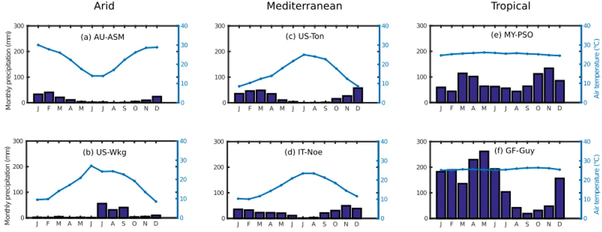
FLUXNET is a network of micrometeorological measurements. It includes more than 800 active and historic flux measurement sites spread across most of the world’s climatic regions and representative biomes (Baldocchi et al., 2001). Six FLUXNET sites were selected from a total of 212 sites in the FLUXNET2015 dataset updated in November 2016. The sites were filtered progressively using the following four criteria: (1) yearlong snow-free conditions (50 sites); (2) data availability of surface energy fluxes and volumetric soil moisture content measurements over multiple years (12 sites); (3) contrasting climate types and (4) biomes (6 sites, Figure 2.1). Table 2.1 summarizes the main characteristics of the study sites, which were grouped, according to the Köppen-Geiger climate classification, as arid, mediterranean, and tropical climates. On the other hand, biome type was grouped according to the In-ternational Geosphere-Biosphere Programme (IGPB) as evergreen needleleaf forest (ENF), grassland (GRA), woody savanna (WSA), closed shrubland (CSH), and evergreen broadleaf forest (EBF).

The sites show mean annual precipitation, ranging from 306 mm at the arid AU-ASM site to 3041 mm at the tropical GF-Guy site (Table 2.1). The mean annual air temperatures range from 15.6 to 25.7◦C (Table 2.1) The AU-ASM site is covered with a mulga savanna woodland at the southern end of the North Australian tropical transect (Hutley et al.,2011). At this site, 70% of its annual precipitation occurs during the summer months (December-February) and 85% falls throughout the monsoon season (November-April). The mean monthly temperature can range from 13◦C in June-July to 33◦C in January (Figure 2.2a). The other arid site, US-Wkg, exhibits a drastic seasonality in precipitation patterns (Figure 2.2b), with 70% of the annual precipitation taking place during the summer months from July to September

(30)

120 o_{W 90}o_{W 60}o_{W 30}o_{W 0}o₃₀o_{E 60}o_{E 90}o_{E 120}o_E 40 o_N 30 o_N 20 o N 10 o_N 0 o 10 o S 20 o_S 30 o_S

Figure 2.1: Location of the FLUXNET study sites. Alice Springs (AU-ASM) in Australia; Walnut Gulch Kendall Grasslands (US-Wkg) and Tonzi Ranch (US-Ton) in the United States; Arca di Noe-Le Prigionette (IT-Noe) in Italy; Pasoh Forest Reserve (MY-PSO) in Malaysia; Guyaflux (GF-Guy) in French Guiana.

Table 2.1: Main characteristics of the study sites.

AU-ASM US-Wkg US-Ton IT-Noe MY-PSO GF-Guy

Latitude (◦) −22.28 31.74 38.43 40.61 2.97 5.28

Longitude (◦₎ _133.20 _−109.94 _−120.97 _8.15 _102.31 _−52.92

Altitude (m) 606 1530 177 25 150 48

Climate classification1 _Bsh _BSk _Csa _Csa _Af _Af

Biome type2 _ENF _GRA _WSA _CSH _EBF _EBF

MAP (mm)3 ₃₀₆ ₄₀₇ ₅₅₉ ₅₈₈ ₁₈₀₄ ₃₀₄₁

MAT (◦C)3 _20.0 _15.6 _15.8 _15.9 _25.3 _25.7

Data period of simulation 2011-2014 2011-2014 2003-2014 2004-2014 2003-2009 2004-2014

1_{Köppen-Geiger climate classification: hot semiarid (Bsh), cold semiarid (BSk).}

2_{Biome types according to IGBP land cover classification: evergreen needleleaf forest (ENF), grassland}

(GRA), woody savanna (WSA), closed shrubland (CSH), evergreen broadleaf forest (EBF).

3_{Mean annual precipitation (MAP) and mean annual air temperature (MAT).}

because of the annual cycle of the North American monsoon (Adams and Comrie,1997). The land is covered mainly by a diverse mosaic of native grassland species replaced progressively by Lehman lovegrass starting in 2006 (Moran et al.,2009). The US-Ton mediterranean site has a mean annual precipitation of 559 mm, with 80% of it concentrated from November to April and with dry and warm conditions during the summer months from July to September (Figure 2.2c). Land cover is classified as an oak savanna woodland (dormant in winter and active in spring and summer) interspersed with grassland and forbs (mainly active during the rainy winter periods) (Baldocchi et al., 2004). The other mediterranean site is in Italy, IT-Noe, and displays a similar behavior compared to the US-Ton site in terms of annual temperatures. Precipitation mainly occurs during Spring and high water deficit is observed from May through September. Intense storms provide significant runoff and low water storage during fall (Marras et al., 2011). The main species of vegetation are juniper and lentisk with variable-sized patches of bare ground (Marras et al., 2011). The MY-PSO tropical site has a mean annual precipitation of 1804 mm, which is less than other regions of Peninsular

(31)

Malaysia (Noguchi et al., 2003). Rainfall peaks in March and April and from October to December (Figure 2.2e). Monthly air temperature does not show seasonality and remains uniform around 27◦C (Figure 2.2e). The area is covered by a mixed dipterocard forest with a continuous canopy height of around 35 m and some emergent trees surpassing 45 m (Kosugi et al.,2012). The other tropical site, GF-Guy, presents intense precipitation during December-February and April-July due to the north-south movement of the Inter-Tropical Convergence Zone (Bonal et al.,2008). This site is located in a tropical wet forest with a mean tree height of 35 m and emerging trees exceeding 40 m (Bonal et al.,2008).

J F M A M J J A S O ND 0 100 200 300 M o n th ly p re c ip it a ti o n ( m m ) 0 10 20 30 40 A ir t e m p e ra tu re ( °C ) J F M A M J J A S O ND 0 100 200 300 M o n th ly p re c ip it a ti o n ( m m ) 0 10 20 30 40 A ir t e m p e ra tu re ( °C ) J F M A M J J A S O ND 0 100 200 300 M o n th ly p re c ip it a ti o n ( m m ) 0 10 20 30 40 A ir t e m p e ra tu re ( °C ) J F M A M J J A S O ND 0 100 200 300 M o n th ly p re c ip it a ti o n ( m m ) 0 10 20 30 40 A ir t e m p e ra tu re ( °C ) J F M A M J J A S ON D 0 100 200 300 M o n th ly p re c ip it a ti o n ( m m ) 0 10 20 30 40 A ir t e m p e ra tu re ( °C ) J F M A M J J A S O N D 0 100 200 300 M o n th ly p re c ip it a ti o n ( m m ) 0 10 20 30 40 A ir t e m p e ra tu re (° C ) (a) AU-ASM (b) US-Wkg (c) US-Ton (d) IT-Noe (f) GF-Guy (e) MY-PSO

Arid Mediterranean Tropical

Figure 2.2: Mean monthly air temperature and precipitation for the studied periods, sorted according to climate type. Arid sites: (a) AU-ASM, (b) US-Wkg; mediterranean sites: (c) US-Ton, (d) IT-Noe; tropical sites: (e) MY-PSO, (f) GF-Guy.

2.1.2 Data

Micrometeorological forcing and validation data were both retrieved from FLUXNET2015 dataset (www.fluxnet.fluxdata.org) at 30-min time steps. The forcing data consisted of these seven atmospheric variables needed to pilot both SVS and CLASS: air temperature (◦C), precipitation (kg m−2 s−1), downward shortwave radiation (W m−2), downward longwave radiation (W m−2), wind speed (m s−1), surface pressure (Pa), and specific humidity (kg kg−1). Specific humidity was estimated as a function of relative humidity and air temperature followingGill(2016). FLUXNET2015 data are gap-filled with a combination of autocorrelation gap-filling techniques (Reichstein et al., 2005) and downscaled ERA-interim data (Vuichard and Papale,2015).

The surface energy fluxes to be evaluated are the latent heat flux (LE), sensible heat flux (H), net radiation (R_n), and soil heat flux (G). They were gap-filled using autocorrelation filling techniques (Reichstein et al.,2005). The turbulent fluxes (LE and H) were measured using the eddy-covariance technique (Moncrieff et al., 1997). They were also adjusted in the FLUXNET2015 dataset by an energy balance closure correcting factor ( (R_n− G)/(H + LE)

(32)

). The factor avoid changes in the heat storage in the ecosystem. It was calculated at 30-min time intervals and applied only when energy closure fell outside 1.5 times the interquartile interval and when all the terms were available. Following similar studies ofBlyth et al.(2010) andAlves et al.(2019), a daily energy balance closure filter was applied in order to guarantee a proper observed surface energy balance closure. The daily filter consisted of discarding days for which the error in energy balance closure exceeded 10%. The percentage of the data accepted is the following: AU-ASM (43.2 %), US-Wkg (17.3 %), US-Ton (11.2 %), IT-Noe (29.4%), MY-PSO(91.6%), GF-Guy was not filtered because observations of G were not available. Observed volumetric soil water content corresponds to the topsoil layer, typically between 5 and 10 cm. It was also gap-filled using autocorrelation filling techniques (Reichstein et al., 2005). Soil moisture observations were derived from electrical property of the soil. More exactly, theta ML2-X probes (Delta-T Devices) were deployed at US-Ton (Miller et al.,2007), Stevens Water Hydra Probe sensors at US-Wkg (Keefer et al.,2008); reflectometry probes at AU-ASM (CS605 and TDR100 Campbell Scientific (Cleverly et al.,2013)), at IT-Noe (CS616-L Campbell Scientific, (Marras et al.,2011)), at MY-PSO (CS615 and CS616, Campbell Scientific (Kosugi et al.,2012)), and at GF-Guy (TRIME FM3; Imko, Ettlingen (Bonal et al.,2008)). 2.1.3 Land surface models

The CLASS model

CLASS was initially conceived in response to the perceived need for more soil thermal and moisture layers and for a separate treatment of vegetation canopy within the Canadian Global Circulation Model (Verseghy, 1991; Verseghy et al., 1993). It has been under continuous development, as evidenced in Verseghy et al. (2017), Wu et al. (2016), von Salzen et al. (2013), Bartlett et al.(2003), andVerseghy (2000). Each grid cell in CLASS may be divided into subareas of (1) bare soil, (2) vegetation over the soil, (3) vegetation over snow, and (4) snow over soil. The vegetation canopy is treated as a single layer, same for the snowpack. The soil column has the flexibility to handle any number of soil layers to whatever depth the user specifies. The energy fluxes are computed based on the heat conservation equation described in Verseghy et al. (1993). The prognostic evolution of soil water content and the vertical water flow are given by the one-dimensional Darcy and Richards equations, respectively (see Verseghy (1991) for a more detailed description.)

Differences between SVS and CLASS

As shown in Table2.2, SVS and CLASS rely on similar parameterizations to represent several physical processes. However, there are two distinctive differences. One is associated with stomatal resistance, where the photosynthesis module is used in SVS, while an empirical parameterization is used in CLASS. Note that, although not in the version used in this study, CLASS can be coupled to a similar photosynthesis module (Melton and Arora, 2014) and

(33)

Table 2.2: Summary of SVS and CLASS main physical processes.

Process SVS CLASS

soil and vegetation turbu-lent fluxes

bulk aerodynamic approach ( Hu-sain et al., 2016)

bulk aerodynamic approach (Verseghy,1991;Verseghy et al.,

1993) soil heat flux residual of net radiation and

tur-bulent fluxes

linear combination of soil tem-peratures (Verseghy,1991) surface (skin) and mean

vegetation temperature

force-restore method ( Bhum-ralkar,1975;Blackadar,1976)

heat diffusion equation

(Verseghy et al.,1993)

transmissivity Beer’s law (Sicart et al.,2004) Beer’s law (Verseghy et al.,1993) canopy interception

ca-pacity

proportional to LAI (Dickinson,

1984)

proportional to LAI (Verseghy et al.,1993)

stomatal resistance 1. empirical parameterization (Jarvis,1976;Noilhan and Plan-ton, 1989; Husain et al., 2016) 2. Photosynthesis module (bio-chemical approach) (Farquhar et al., 1980;Collatz et al., 1991,

1992;Husain et al.,2016)

empirical parameterization (Verseghy et al.,1993)

surface (skin) and mean soil temperature

force-restore method ( Bhum-ralkar,1975;Blackadar,1976)

heat conservation equation (Verseghy,1991)

soil moisture moisture conservation equation

(Husain et al.,2016;Alavi et al.,

2016)

moisture diffusion equation (Verseghy,1991)

soil moisture flux 1-D Darcy’s law (Alavi et al.,

2016)

1-D Darcy’s law (Verseghy,1991) saturated hydraulic

con-ductivity, saturated soil water suction

empirical equation based on soil texture (Brooks and Corey,

1966)

empirical equation based on soil texture (Cosby et al., 1984;

Brooks and Corey,1966) wilting point; field

ca-pacity; saturated values of volumetric water con-tent, hydraulic conductiv-ity, and soil water suction

parameterization from soil tex-ture (Boone et al., 1999;Brooks and Corey,1966)

parameterization from soil tex-ture (Cosby et al., 1984; Soulis et al.,2011)

relationship between soil water content, soil wa-ter potential, and relative permeability

empirical equation (Clapp and Hornberger, 1978; Alavi et al.,

2016)

empirical equation (Clapp and Hornberger, 1978; Verseghy et al.,1993)

vertical water flow 1-D Richards equation (Soulis et al.,2000)

1-D Richards equation

(Verseghy,1991) lateral water flow 1-D Richards equation (Soulis

et al.,2011,2000)

1-D Richards equation (Soulis et al.,2011,2000)

can also have access to a climate vegetation model (von Salzen et al., 2013). The other difference resides in the method used for computing the surface (skin) temperature and the mean temperature of the vegetation and soil components. A one-layer force-restore method is employed in SVS, while CLASS uses a multi-layer heat diffusion equation. Note that a multi-layer Richard’s equation framework for soil moisture is used in SVS and CLASS. The force-restore approach is still used in SVS for its computational efficiency and parsimony (less state variable) in the context of operational forecasting.

2.1.4 Experimental setup

In this study, experiments were performed at point-scale and in offline mode with the MESH modeling platform (Modélisation Environnementale communautaire - Surface Hydrology),

(34)

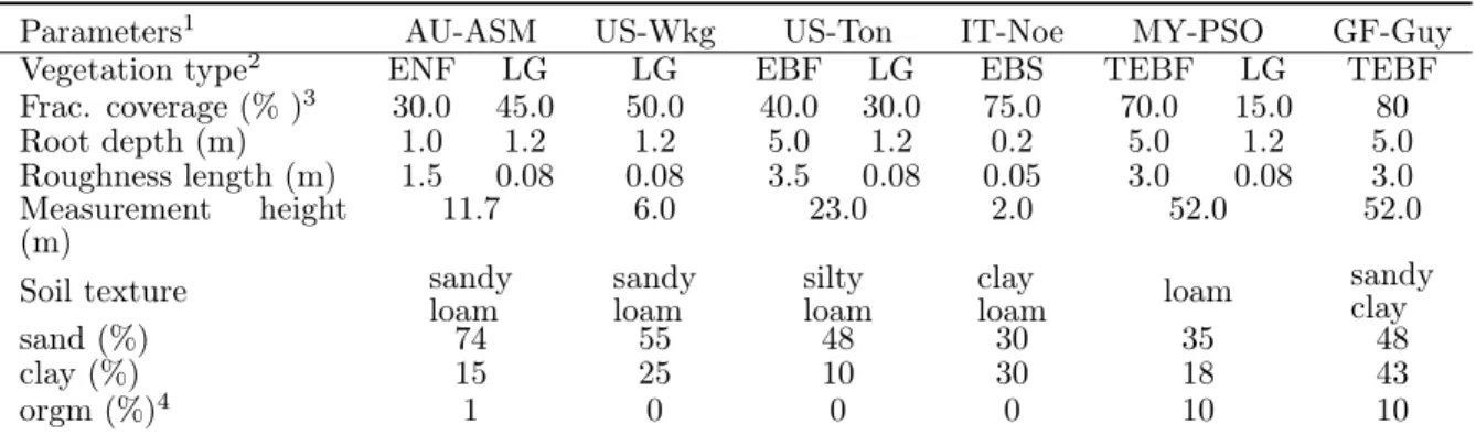
Table 2.3: Parameters for SVS and CLASS models at each FLUXNET site used in this study.

Parameters1 _AU-ASM _US-Wkg _US-Ton _IT-Noe _MY-PSO _GF-Guy

Vegetation type2 ENF LG LG EBF LG EBS TEBF LG TEBF

Frac. coverage (% )3 _30.0 _45.0 _50.0 _40.0 _30.0 _75.0 _70.0 _15.0 ₈₀ Root depth (m) 1.0 1.2 1.2 5.0 1.2 0.2 5.0 1.2 5.0 Roughness length (m) 1.5 0.08 0.08 3.5 0.08 0.05 3.0 0.08 3.0 Measurement height (m) 11.7 6.0 23.0 2.0 52.0 52.0

Soil texture sandy

loam sandy loam silty loam clay loam loam sandy clay sand (%) 74 55 48 30 35 48 clay (%) 15 25 10 30 18 43 orgm (%)4 1 0 0 0 10 10

1_{References for the parameter values: AU-ASM:} _{Cleverly et al.}₍₂₀₁₃_{); US-Wkg:} _{Scott et al.} ₍₂₀₁₀_);

US-Ton: Baldocchi et al. (2004); IT-Noe: Marras et al. (2011); MY-PSO: Kosugi et al. (2012),

Yamashita et al. (2003); GF-Guy: Bonal et al.(2008).

2_{Vegetation type for SVS and CLASS: ENF: evergreen needleleaf forest; LG: long-grass; EBF:}

evergreen broadleaf forest; EBS: evergreen broadleaf shrub; TEBF: tropical evergreen broadleaf forest .

3_{Note: the remainder non-vegetative percentage corresponds to bare ground.} 4_{orgm: organic matter (only used in CLASS).}

which is ECCC’s community environmental modeling system (Pietroniro et al.,2007). MESH allows different LSMs and hydrologic routing models to coexist within the same modeling framework. Although the final goal of MESH is to forecast water discharge at the watershed scale, it is also possible to utilize the stand-alone offline versions of SVS and CLASS, which are the two current LSMs integrated into MESH. A technical description of MESH can be found inPietroniro et al. (2007) and www.wiki.usask.ca/display/MESH. MESH, including the SVS and CLASS codes, is available at www.wiki.usask.ca/display/MESH/Interim+releases. Three time steps were specified in the models: (1) the input time step was set as 30-min for each model; (2) the model time step was defined as 5-min for SVS and 30-min for CLASS (a test carried out with CLASS for a time step of 5-min revealed almost the same results as those obtained at 30-min) ; and (3) the output time step was fixed as 30-min for both models. The soil was divided into seven layers with depths from the top to the bottom equal to 10, 35, 85, 160, 235, 310, and 410 cm. Soil texture was assumed constant in the vertical direction since information at multiple depths was not available in the literature (Table 2.3).

The soil texture parameters used at each site (Table 2.3) are provided to both models, except for the organic matter (orgm), which is used only by CLASS.

Vegetation associated parameters are defined in the look-up tables of each model. As shown in Table2.3, both models account for the same vegetation type. For simplicity shown treating lateral water fluxes, the grid was considered perfectly flat at all sites.

(35)

Both models were set up with the same initial soil moisture and temperature conditions. Soil temperature for each layer was initialized with the yearly mean temperature. Soil moisture for each layer was initialized at 50% of saturation. To account for an equilibrium in the prognostic variables at each site (spinup), the first year of meteorological input was replicated ten times.

2.2 Methodology for the SVS evaluation under snow condition

2.2.1 ESM-SnowMIP Dataset

The meteorological and evaluation datasets from the Earth System Model-Snow Model Inter-comparison Project (ESM-SnowMIP), an international coordinated modelling effort to in-vestigate snow schemes (Krinner et al., 2018), are used here. The dataset is described in great detail by Ménard et al. (2019) and can be found on the PANGEAE repository (https://doi.pangaea.de/10.1594/PANGAEA.897575). It includes post-processed and quality-controlled data from ten sites that total 136 years of in-situ measurements at 60-min time steps. The measurements are grouped as the meteorological forcing and evaluation datasets.

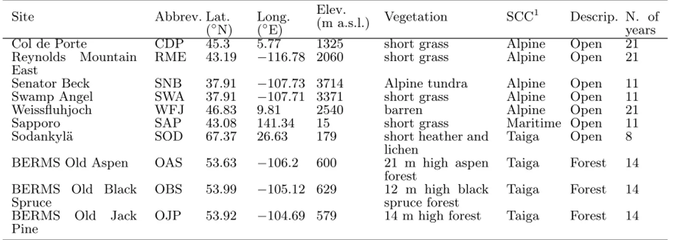
Table 2.4: Main characteristics of the study sites.

Site Abbrev. Lat. (◦N) Long. (◦E) Elev. (m a.s.l.) Vegetation SCC 1 Descrip. N. of years Col de Porte CDP 45.3 5.77 1325 short grass Alpine Open 21 Reynolds Mountain

East

RME 43.19 −116.78 2060 short grass Alpine Open 21 Senator Beck SNB 37.91 −107.73 3714 Alpine tundra Alpine Open 11 Swamp Angel SWA 37.91 −107.71 3371 short grass Alpine Open 11 Weissfluhjoch WFJ 46.83 9.81 2540 barren Alpine Open 21 Sapporo SAP 43.08 141.34 15 short grass Maritime Open 11 Sodankylä SOD 67.37 26.63 179 short heather and

lichen

Taiga Open 8 BERMS Old Aspen OAS 53.63 −106.2 600 21 m high aspen

forest

Taiga Forest 14 BERMS Old Black

Spruce

OBS 53.99 −105.12 629 12 m high black spruce forest

Taiga Forest 14 BERMS Old Jack

Pine

OJP 53.92 −104.69 579 14 m high forest Taiga Forest 14

1

Snow cover classification (SCC,Sturm et al.(1995)).

The main characteristics of the study sites are given in Table 2.4. Seven out the ten sites are open, while three are forested. According to the Snow Cover Classification (SCC, Sturm et al. (1995)), five sites are alpine, four are taiga, and one is maritime (Table 2.4). Most of the open sites are covered with short grass, while SNB is covered with alpine tundra and SOD with short heather and lichen. The mean canopy heights at OAS, OBS, and OJP reach 21, 12, and 14 m, respectively. These latter three sites are located in the Canadian boreal biome and form the Boreal Ecosystem REsearch and Monitoring Sites (BERMS, see Bartlett et al. (2006)).

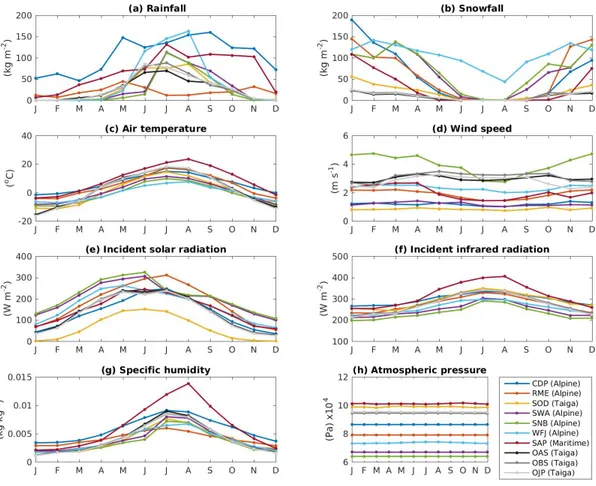
A detailed description of each site can be found in Ménard et al.(2019). Figure 2.3 provides an overview of the prevailing climatology at each location. Most of the sites registered snowfall

(36)

from September to June, except for WFJ that is exposed to snowfall yearlong (Figure 2.3b). SOD and the three BERMS sites (OAS, OBS, OJP) show the lowest snowfall accumulation. At these sites, rainfall declines progressively from September to December and becomes more prevalent between March and May. CDP shows high rainfall rates in winter and RME, the driest condition. SOD and the BERMS sites exhibit the lowest air temperatures between December and February, with mean values close to −15◦C. WFJ, SNB, and SWA manifest the most extended negative temperatures, between 0 and −5◦C from October to April. SAP, CDP and RME are the warmest locations, recording air temperatures close to 0◦C from November to March (Figure 2.3c). All sites present wind speed between 1 and 2 m s−1, except for SNB that reports values around 5 m s−1 from December to April (Figure 2.3d). SWA and SNB report the highest monthly mean solar radiation (between 100 and 150 W m−2 from October to February, Figure 2.3e), and SOD, the lowest values during the same period (between 0 and 50 W m−2, Figure 2.3e). Infrared radiation ranges from 200 to 300 W m−2, from November to April (Figure 2.3f). Specific humidity oscillates between 0.001 and 0.004 kg kg−1 over the same months (Figure 2.3g). Atmospheric pressure shows no seasonality and ranges between 62 kPa at SOD and 102 kPa at SAP (Figure 2.3h). It is obviously inversely proportional to the site elevation.

As already mentioned, the evaluation subset includes observations of snow water equivalent (SWE), snow depth, surface albedo, surface temperature, and soil temperature. SWE and snow depth were manually measured at all sites on a weekly to monthly basis, over a predefined area around the meteorological stations. Daily automatic observations of snow depth are reported at all sites, but daily automatic SWE is available at only a few sites. Daily effective albedo is available at five locations. They were calculated from the incident and reflected observed solar radiation using the method of Morin et al. (2012). Surface temperature is available at the same five sites, and was recorded hourly and derived from the measurements of the re-emited longwave radiations, except at SNB where infrared temperature sensors were deployed.

2.2.2 Experimental setup

A similar setup as in Section 2.1.4 is used in this part of the experiments. That means point-scale experiments relied on the stand-alone implementation of SVS within the MESH modelling platform.

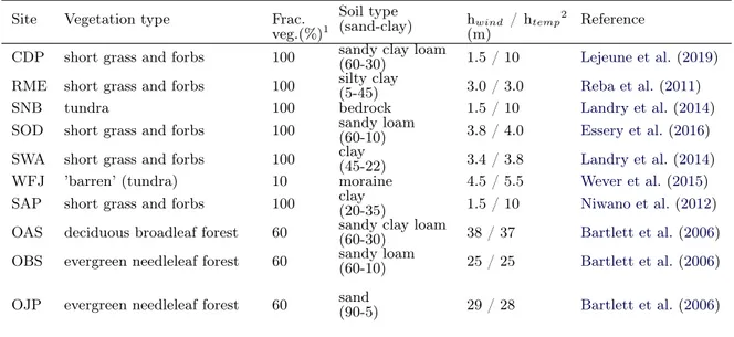
Forcing data needed to drive SVS are air temperature (◦C), precipitation rate (kg m−2 s−1), downward shortwave radiation (W m−2), downward longwave radiation (W m−2), wind speed (m s−1), surface pressure (Pa), and specific humidity (kg kg−1). Liquid and solid precipitation are provided in the ESM-SnowMIP forcing dataset. Besides, a number of parameters depicting the vegetation type, fraction of vegetation, soil type, and measuring height for wind speed, air temperature, and humidity are set according to the available literature for each location

(37)

Figure 2.3: Monthly mean (a) rainfall, (b) snowfall, (c) air temperature, (d) wind speed, (e) solar radiation, (f) infrared radiation, (g) specific humidity, and (h) atmospheric pressure at the ESM-SnowMIP sites.

(Table 2.5). Some supplemental parameters are associated with each vegetation type in the SVS look-up tables.

A 5-min model time step is used for all simulations, as this is a regular time step for the operational use of SVS. Model outputs are averaged to 60 min in order to be consistent with the observations. Albedo was averaged between 9:00 and 15:00 local time. At each site, the first year is replicated five times for the model spinup. Snowpack overlaying bare ground and low vegetation was used for the evaluation at CDP, RME, SNB, SWA, WFJ, SAP, and SOD sites, where as the subcanopy snowpack was used for the evaluation at BERMS sites.

2.2.3 Crocus snow model simulations

As a strategy to better interpret SVS results, outputs from the Crocus snowpack model are also considered in some specific cases. Interpretations will not focus on comparing SVS and Crocus,