HAL Id: tel-00142413
https://pastel.archives-ouvertes.fr/tel-00142413
Submitted on 18 Apr 2007HAL is a multi-disciplinary open access archive for the deposit and dissemination of sci-entific research documents, whether they are pub-lished or not. The documents may come from teaching and research institutions in France or abroad, or from public or private research centers.
L’archive ouverte pluridisciplinaire HAL, est destinée au dépôt et à la diffusion de documents scientifiques de niveau recherche, publiés ou non, émanant des établissements d’enseignement et de recherche français ou étrangers, des laboratoires publics ou privés.
METASTABLE HELIUM
José Carlos Viana Gomes
To cite this version:
José Carlos Viana Gomes. THERMOMETRY AND COHERENCE PROPERTIES OF A ULTRA-COLD QUANTUM GAS OF METASTABLE HELIUM. Atomic Physics [physics.atom-ph]. Université Paris Sud - Paris XI, 2007. English. �tel-00142413�
INSTITUT D’OPTIQUE TH´
EORIQUE ET APPLIQU´
EE
LABORATOIRE CHARLES FABRY
UNIVERSIT´
E PARIS XI
U.F.R. SCIENTIFIQUE D’ORSAY
TH `ESE
pr´esent´ee pour obtenir
le GRADE de DOCTEUR EN SCIENCES DE L’UNIVERSIT ´E PARIS XI ORSAY
par
Jose Carlos VIANA GOMES
Sujet :
THERMOM´
ETRIE ET PROPRI´
ET´
ES DE COH´
ERENCE
D’UN GAZ QUANTIQUE ULTRA-FROID D’H´
ELIUM M´
ETASTABLE
A soutenir le 9 fevrier devant la Commission d’examen : M. C. WESTBROOK Directeur de th`ese M. M. BELSLEY Directeur de th`ese
M. V. LORENT Rapporteur
M. J. MENDON ¸CA Rapporteur
M. O. DULIEU Examinateur
M. J. FERREIRA Examinateur M. D. BOIRON Membre invit´e
Aos meus
pais
Ces travaux de thèse ont été réalisés au Laboratoire Charles Fabry de l'Institut d'Optique. Je remercie son directeur, Pierre CHAVEL, de m'y avoir accueilli.
Je remercie Alain ASPECT pour m'avoir accepté dans son équipe, et pour son amitié et sa disponibilité au cours de tout mon séjour à Orsay. C'était un privilège de pouvoir le connaître, entendre ses leçons de physique, toujours très riches et perspicaces.
Je remercie Chris WESTBROOK, mon directeur de thèse à Orsay, ses enseignements, son enthousiasme et l'énergie qu'il a toujours mis dans notre activité scientifique, ses mots d'incitation et d´encouragement ainsi que d'avoir été toujours disponible pour aider quand il y avait des problèmes, scientifiques ou autres.
Devo também um agradecimento muito especial ao Michael BELSLEY (Mike), o meu (desde sempre!) orientador em Braga. O Mike foi, sem dúvida, a pessoa que mais me influenciou em todo o meu percurso académico. Foi ele que, em grande medida, soube mostrar o prazer que há em “fazer” Física, o tornar simples e inteligível fenómenos que, à primeira vista, pareciam muito mais complicados. É sempre um prazer e um privilégio, poder discutir (e aprender) Física com o Mike, seja no “referencial do laboratório” ou no do “papel e lápis”.Ele dizia-me, há dias, que a função de um professor de Física era ensinar os alunos a pensar: não conheço quem o faça melhor! Espero que guarde sempre a vontade e a motivação para continuar a ensinar Física.
O Mike é também o primeiro responsável pela minha ida para Orsay para doutoramento, pois sempre me incentivou a “sair de Braga” para conhecer outras realidades, porventura mais competitivas: foi ele que me levou a contactar o Alain para fazer o doutoramento em Orsay. Muito obrigado Mike!
Je remercie Vincent LORENT qui a bien voulu accepter de faire un rapport de ce manuscrit et pour le temps qu'il a consacré à sa relecture. Je le remercie aussi pour m'avoir aidé dans la compilation finale des petites erreurs qu'il contenait. Agradeço igualmente a José TITO
MENDONÇA por ter aceite amavelmente ser relator da minha tese.
Je remercie également Olivier DULIEU pour avoir accepté de participer à mon jury.
Agradeço igualmente a João ALVES FERREIRA por ter aceite participar no júri da minha tese e pela sua consideração e amizade.
Pendant tout le temps de ma thèse, le vrai 'gluon' qui liait toutes les personnes qui sont passées par la manip d’Hélium, qui était toujours prêt pour nous aider et auquel nous faisions appel chaque fois que le ciel semblait tomber sur nos têtes, a été Denis BOIRON. Il m'est difficile d'exprimer (surtout en Français !) le profond sentiment de gratitude que j'ai pour Denis (ça augmente chaque fois que je pense au nombre de fois qu'il a lu et corrigé le texte de ma thèse!). Il a été, certainement, la personne avec laquelle j'ai le plus appris de Physique (des condensats de Bose-Einstein, mais pas seulement) pendant ma thèse. Il a toujours essayé de répondre à toutes nos questions, même les plus 'stupides'. En plus, Denis a toujours été un très bon ami. Je le remercie aussi pour l'intérêt constant qu'il a toujours porté à mon travail. Merci beaucoup Denis!
Dans le groupe de pionniers dans la condensation de l'Hélium il y avait Antoine BROWAEYS, Alice ROBERT et aussi Olivier SIRJEAN (c'est lui qui a obtenu le premier condensat!). C'est Olivier qui m'a enseigné, avec patience, le fonctionnement de la manip et ‘à comprendre’ ses humeurs (de la manip, bien sûr!) pour mieux la contrôler. C’est aussi avec Olivier que j'ai passé beaucoup de ma période initiale de thèse, au laboratoire, à résoudre des problèmes quotidiens, à obtenir et à traiter les résultats. À lui, mon sincère merci pour tout.
Un mot de remerciement aussi à Antoine qui, après être revenu à Orsay, a toujours eu une énorme disponibilité pour nos questions sur l'expérience, toujours avec amitié.
même fini sa thèse avant moi, le malin!), Martijn SCHELLEKENS (le plus célèbre évangéliste de Root) et Aurélien PERRIN. De tous je garde une mémoire pleine de moments de camaraderie et, surtout, de grande amitié.
Finalement, déjà dans la période finale de ma thèse, nous avons été rejoints par Valentina KRACHMALNICOFF et Hong CHANG qui ont réussi très rapidement, avec l'aide de Denis, Martijn et Aurélien, à s'adapter aux caprices de la manip. Je suis très impressionné par les beaux résultats qu'ils ont aidé à obtenir dans l'expérience de corrélation des fermions: bravo Valentina et Hong!
Si les choses fonctionnaient aussi bien dans les manips, c'est grâce à nos électroniciens André VILLING et Frédéric MORON. Je les remercie chaleureusement pour leur compétence, leur disponibilité et tout leurs précieux enseignements d'électronique. Tive também a sorte de
poder contar com a ajuda do José CUNHA, o nosso “electrónico” em Braga. Para além da sua grande competência pude também usufruir da sua amizade.Espero poder aprender ainda muita electrónica com ele!
Il est très difficile de parler de toutes les personnes que j'ai eu le plaisir de connaître à Orsay pendant ma thèse. Je garde le souvenir de l'ambiance très conviviale et amicale dans notre groupe. Les discussions (pas toujours de physique!!!) avec Isabelle, les 'coffee breaks' ('tee breaks'?) avec Rob ou les conversations à la rentrée chez nous à la Cité Internationale
Universitaire de Paris (CIUP) avec Andrès me manquent déjà. Il faut encore rajouter des noms
dans mes remerciements (j'espère n'oublier personne!): Guillaume, Christine, David S., Jérôme, Fabrice, Thorsten, Marie, Simon, Mathilde, Joseph, Jocelyn, David C., Yann, Felix, Jean-François, Jean-Baptiste, Gaël… et encore Philippe, Nathalie, Ronald, Carlos, Laurent, Sadiqali… merci à tous!
Paris & Casa de Portugal. Muitas linhas seriam necessárias para citar todas as pessoas com quem travei amizade na Casa de Portugal na CIUP. Desde logo a Irina, mas também o meu grande amigo Nuno SILVA, que tantas vezes me aturou e ajudou durante todos estes anos em Paris. Muito obrigado Nunão! Mas houve mais quem me aturasse! Um grande obrigado aos meus amigos Inês, Alberto, Patrícia, Joana, Alexandro... Agradeço também, claro, à Casa de Portugal por me ter acolhido. Espero que tenha as suas portas sempre abertas para acolher jovens portugueses (e de outras nacionalidades!) que queiram prosseguir com os seus estudos em Paris.
Braga. Agradeço também aos meus colegas do Dep. Física o incentivo que me deram. Entre eles, um agradecimento especial aos meus amigos Teresa, Anabela, Luís Vieira, Nuno Peres e Eduardo. Também em Braga houve quem me aturasse: a Lau, o Chico, a Anabela, o Luís, a Clara, o Óscar, o Tozé... A todos o meu muito obrigado.
Por fim, tenho que agradecer à minha família, os meus pais, o meu irmão, a Sofia, os meus sobrinhos, a Nanda, por todo o enorme apoio que sempre me deram e a paciência que sempre tiveram comigo e para com o meu trabalho. Depois de estar em Paris mais de três anos, longe de todos, quando voltei ainda tive muitas vezes que lhes dizer “não posso... tenho que ficar a trabalhar na tese...”!
Por fim, um agradecimento muito muito especial à Irina, a companheira com quem partilhei a minha vida, todas as pequenas vitórias mas também as grandes derrotas, em todos estes anos. Obrigado por teres estado sempre presente, mesmo quando estivemos separados por muitas centenas de quilómetros! Nunca desistas do sonho!
1 Bose-Einstein Condensation of Metastable Helium: the
ap-paratus. 29
1.1 Road map to achieve BEC in He∗. . . 31 1.2 Producing a metastable helium Bose Einstein condensate. . . 33 1.2.1 The magnetic trap and evaporative cooling. . . 33 1.2.1.1 Trapping neutral atoms with a magnetic field. 34 1.2.1.2 Trap geometry and configurations. . . 36 1.2.1.3 Evaporative cooling. . . 40 1.2.2 The bias field fluctuation. Effort towards its stabilization. 43 1.2.3 From the helium bottle to a cloud of ultra-cold He∗atoms
in the magnetic trap. . . 49 1.3 Experimental readout. . . 58 1.3.1 The micro-channel plate. . . 58 1.3.2 Saturation effects and the counting and analog
detec-tion modes. . . 59 1.3.3 The atoms’ time of flight signal. . . 60 1.3.4 The ion signal. . . 62
1.3.4.1 The two and three-body Penning ionization processes. . . 62 1.3.5 The complete scheme of the detection system. . . 67 1.3.6 The calibration of the MCP detection system. . . 67
1.3.6.1 The difficult calibration of the number of atoms in a TOF signal. . . 67 1.3.6.2 The detection sensitivity for the counting mode. 70 2 The ultra-cold non-degenerate ideal gas. 71 2.1 An ideal gas cloud confined in a harmonic trap. . . 72 2.1.1 Atomic density in thermal equilibrium. . . 72 2.1.1.1 The critical temperature. . . 77 2.1.1.2 The finite size effect importance in the cloud
density close to the critical transition point. . 79 2.1.2 The critical atomic peak density. . . 81 2.1.3 The finite size SCA for spatially integrated density
2.1.4 The momentum distribution. . . 85
2.2 Time of Flight: theoretical description. . . 87
2.2.1 Ballistic expansion of an ideal gas under the effect of a gravitational field. . . 87
2.2.1.1 Quantum mechanical flux. . . 88
2.2.1.2 Time evolution of a h.o. wave function in free fall . . . 89
2.2.2 Ballistic expansion in the far field and long fall ap-proximations. . . 92
2.2.2.1 The far field approximation. . . 92
2.2.2.2 The long fall approximation. . . 93
2.2.2.3 The TOF signal for the ideal gas. . . 93
2.2.2.4 Snap-shot measure of the cloud’s density. . . 94
3 Hanbury Brown and Twiss effect in an expanding cold of non-interacting atoms. 97 3.1 The Hanbury Brown and Twiss experiment. . . 99
3.1.1 The transversal coherence length and time coherence of a wave field. . . 99
3.1.2 The HBT experiment. . . 104
3.1.2.1 Laser light. . . 104
3.2 Correlation functions in a non-interacting atomic gas. . . 106
3.2.1 Definitions . . . 106
3.2.1.1 Correlation functions defined in coordinate space. . . 106
3.2.1.2 The influence of the ground state population. 109 3.2.1.3 Correlation functions in the momentum space. 110 3.3 Correlation functions in a harmonic trap. . . 111
3.3.1 At equilibrium in the trap . . . 111
3.3.2 Integrated signals . . . 116
3.4 Correlations in a harmonically trapped cloud after expansion . 119 3.4.1 Detection: Snap-shot and flux measurement. . . 119
3.4.2 Second order correlation function of a expanded cloud in a snap shot measurement. . . 120
3.4.3 Intensity-intensity correlation function of a expanded cloud. . . 121
3.4.3.1 Explicit calculation of the flux correlation func-tion within the far field and long fall approx-imations. . . 122
3.4.4 Conclusion. . . 125
3.5 The HBT experiment with He∗. . . 126 3.5.1 State of the art on HBT measures with massive particles.126
3.5.2 The HBT experiment with He∗. . . 127 3.5.2.1 The delay line detector. . . 127 3.5.2.2 The bunching contrast in function of the pixel
size. . . 128 3.5.3 A simple derivation of the signal-to-noise ratio. . . 129 3.5.4 Exact results for the SNR in the high temperature limit.131 3.5.5 The experimental results. . . 132 3.5.6 Conclusion. . . 133 4 Thermometry with ions and atoms: theoretical
preliminar-ies. 135
4.1 Introduction . . . 135 4.2 The ion signal. . . 137 4.2.1 Ion signal during the last evaporative ramp. . . 138 4.2.2 Simulation of the ion signal in the last evaporative ramp.140 4.2.2.1 Ion signal in the non-degenerate cloud. . . 141 4.2.2.2 Ion flux in degenerate cloud. . . 141 4.2.3 The cloud’s populations rate equations. . . 146 4.2.3.1 The atom losses due to inelastic collisions. . . 146 4.2.3.2 Atom losses due to the evaporative cooling. . 146 4.2.3.3 Numerical simulation: overview. . . 150 4.2.3.4 Presentation of some results. . . 151 4.2.4 Critical curve. . . 154 4.2.4.1 The critical curve in the simulated results. . . 154 4.2.4.2 Empirical determination of the critical
tran-sition point. . . 154 4.2.4.3 The critical curve for real data. . . 160 4.2.4.4 Further characterization of the ion signal. . . 162 4.2.5 Conclusion. . . 163 4.3 TOF based thermometry for non degenerate atomic clouds. . 165 4.3.1 Inclusion of interatomic interactions. . . 165 4.3.2 Atomic density matrix in the Hartree-Fock mean field
approximation. . . 166 4.3.2.1 Redefinition of the chemical potential to
ac-count for the interaction energy at the cloud’s center. . . 166 4.3.2.2 Further simplifications towards the derivation
of n(r). . . 167 4.3.2.3 The classical phase space distribution
func-tion f (r, p). . . 171 4.3.3 The time of flight of a thermal cloud. . . 172
4.3.4 The cloud’s hydrodynamical expansion: thermometric
correction. . . 174
4.3.4.1 The Knudsen criterion . . . 175
4.3.4.2 Description using the Boltzmann-Vlasov ki-netic equation. . . 176
4.3.4.3 Hydrodynamical expansion and temperature correction. . . 178
4.3.5 Conclusion. . . 180
5 The cloud thermometry and the determination of the He∗scattering length. 181 5.1 Introduction. . . 181
5.2 Determination of the scattering length. . . 184
5.2.1 High order corrections for the ion flux signal in the non-degenerate case. . . 185
5.2.1.1 Ion flux signal at Z = 1. . . 186
5.2.2 The data analysis procedure. . . 186
5.2.3 Variation of the fitted temperature with a. . . 187
5.2.3.1 Experimental procedure. . . 189
5.2.4 Sorting data at Z = 1. . . 192
5.2.5 The found value for a. . . 196
5.2.5.1 Obtained result. . . 196
5.2.5.2 Error estimation. . . 196
5.2.6 Final remarks on the determination of a. . . 198
5.3 Revisiting the problem of the determination of the s-wave scat-tering length. . . 200
5.3.1 The data dispersion and the bias fluctuation. . . 200
5.3.1.1 Dispersion produced by the inclusion of ther-mal clouds. . . 201
5.3.1.2 Dispersion due to the degenerate clouds. . . . 203
5.3.2 The problem of sorting data at Z = 1. Overview to the χ2-maps. . . . 204
5.3.3 The problem of the initial guess for a. . . 208
5.3.4 The results. . . 209
5.3.4.1 The found a in function of the fugacities. . . . 209
5.3.4.2 The found a dependence on temperature for different fugacities. . . 209
5.3.5 Final remarks. . . 211
5.4 The systematic error on the measurement of the scattering length. . . 215
5.4.1 The slow trap switch-off scenario for the thermal cloud release. . . 217
5.4.2 The thermal cloud’s trap relaxation time for obtaining
a = 7.5 nm. . . 220
5.4.3 The influence on the measure of β and L of a slow release of the BEC. . . 220
5.4.3.1 The hydrodynamical slow expansion of the condensate. . . 222
5.4.3.2 Consequences on the determination of β and L. . . 224
5.4.3.3 Consequences on the measurement of a. . . . 226
5.4.4 Conclusion. The Raman transition outcoupling process. 228 A The condensate in the Thomas-Fermi approximation. 230 A.1 The condensed state: Gross-Pitaevskii equation. . . 230
A.2 Thomas-Fermi approximation. . . 231
A.3 The TOF of the BEC. . . 233
A.3.1 The time dependent Gross-Pitaevskii equation. The hydrodynamical equivalent. . . 233
A.3.2 The condensate detected atomic flux. . . 235
A.3.3 The ion flux from a condensate. . . 237
B The condensate and the determination of the ionizing rate constants. 239 B.1 The condensate. . . 239
B.1.1 The pure BEC. . . 239
B.1.2 Chemical potential and cloud’s number of atoms. . . . 241
B.2 The measure of β and L experiment. . . 241
B.2.1 The experimental procedure. . . 241
B.2.2 Obtained results and their analysis. . . 243
B.2.2.1 Analysis and results with a = 12nm . . . 245
B.2.3 Dependence of the fitting result in the scattering length.249 C Mean Field Approximation 251 D Fugacity determination with the χ2 maps 255 D.1 Introduction . . . 255
D.2 The Z − T χ2− maps. . . 256
D.3 Getting the fugacity from a χ2− map. . . 261
D.3.1 χ2-map strategy for finding Z map. . . 262
D.3.2 Definition of the χ2-map criteria for sorting data at T = Tc. . . 263
D.4 Using the semi-ideal model for testing the χ2-map method. . . 265
D.4.1 The analysis of synthesized data at Z = 1. . . 265
Introduction.
En 1925, Albert Einstein a pr´edit que si un gaz id´eal d’atomes bosoniques ´
etait refroidi en-dessous d’une certaine temp´erature, il subirait une transition de phase vers un nouvel ´etat o`u une fraction macroscopique des atomes oc-cuperait le mˆeme ´etat fondamental du syst`eme. Cet effet remarquable est une cons´equence de la statistique des particules identiques de spin entier, qui avait ´et´e r´ecemment d´eriv´ee par lui et Satyendra Nath Bose. Malgr´e cette pr´ediction pr´ecoce, il n’est devenu possible de cr´eer un condensat de Bose-Einstein (CBE) dans un ´echantillon atomique dilu´e que dans les ann´ees 90. Dans ces exp´eriences le gaz est fortement localis´e en position et en impul-sion. Pour ´eviter la formation des ´etats mol´eculaires (et r´eduire les pertes provoqu´ees par les collisions non ´elastiques) l’´echantillon est tr`es dilu´e, des millions de fois moins dense qu’un gaz id´eal `a la pression atmosph´erique et `a la temp´erature ambiante. Les temp´eratures de transition de phase sont alors extrˆemement petites, de l’ordre du microkelvin, ce qui a constitu´e pendant longtemps un d´efi consid´erable.
0.1
L’exp´
erience d’h´
elium m´
etastable.
L’h´elium m´etastable (He∗) a rejoint, en 2001, le groupe des esp`eces ato-miques dilu´ees condens´ees. C’´etait ´egalement la premi`ere fois qu’un CBE a ´
et´e r´ealis´e dans un gaz atomique en dehors de l’´etat fondamental ´electronique. Pour He∗, il s’agit du premier ´etat ´electronique excit´ee de l’h´elium, 23S
1, un
´
etat m´etastable avec un temps de vie de 9000 secondes et une ´energie in-terne de 20 eV. La manipulation optique de l’´echantillon esot assur´ee par une transition ferm´ee vers l’´etat excit´ee 23P
2 `a la longueur d’onde de 1.083 µm.
L’´etat m´etastable a ´egalement un moment dipolaire magn´etique qui permet le pi´egeage magn´etique et le refroidissement ´evaporatif par radiofr´equence. La polarisation magn´etique de l’´echantillon supprime fortement les collisions non ´elastiques entre les atomes d’He∗, ce qui augmente la stabilit´e et la vie de l’´echantillon, et a finalement permis d’atteindre la CBE. Les 20 eV d’´energie interne de l’He∗ sont suffisants pour extraire un ´electron d’une surface m´ etal-lique. Ce fait est employ´e dans la d´etection par temps-de-vol atomique (tdv ),
en lib´erant les atomes du potentiel de pi´egeage et en les laissant tomber sur une galette de micro-canaux (GMC). Ce dispositif fonctionne comme un mul-tiplicateur d’´electrons et produit un signal proportionnel au flux atomique.
Le travail exp´
erimental r´
ealis´
e pendant la th`
ese.
Cette th`ese rend compte du travail exp´erimental effectu´e sur deux sujets dans la manipulation exp´erimentale d’un nuage quantique d’He∗ : i) nous avons mesur´e les param`etres fondamentaux pour d´ecrire les collisions ´ elas-tiques entre atomes d’He∗ (longueur de diffusion a) et les collisions non ´ elas-tiques ionisantes entre deux et trois atomes d’He∗ (constantes d’ionisation `a deux et `a trois corps β et L), ii) nous avons fait une mesure des corr´elations entre He∗ sur le flux atomique. Cette derni`ere exp´erience est conceptuelle-ment ´equivalente `a celle de Robert Hanbury Brown et Richard Twiss (HBT ) avec des photons en 1956, et qui a ´et´e une exp´erience pionni`ere en Optique Quantique. Notre exp´erience a r´ealis´e pour la premi`ere fois la mesure de la fonction de corr´elation de densit´e de particules massives pour un ´echantillon atomique d´eg´en´er´e et non d´eg´en´er´e, confirmant le comportement pr´evu pour la coh´erence du second ordre.
Le gaz d´
eg´
en´
er´
e et le gaz `
a la temp´
erature
cri-tique.
Pour ces exp´eriences, il est tr`es important de caract´eriser le gaz, c’est-` a-dire faire sa thermom´etrie. Elles ont ´et´e effectu´ees avec des CBEs pur (presque `
a T = 0) ou avec des nuages thermiques `a proximit´e de la temp´erature cri-tique. Caract´eriser un nuage atomique condens´e est plutˆot simple, puisque le temps de vol atomique a une signature claire : c’est une parabole inver-s´ee, tr`es bien d´ecrite th´eoriquement dans l’approximation de Thomas-Fermi. Du point de vue exp´erimental, pour cr´eer un CBE pur il suffit de refroidir le nuage atomique jusqu’`a ce qu’aucune composante thermique (c.-`a-d. non-d´eg´en´er´ee) ne reste pi´eg´ee. Ce n’est ´evidemment possible que si le nombre ini-tial d’atomes pi´eg´es au d´ebut du refroidissement est suffisant pour atteindre la d´eg´en´erescence avec un nombre raisonnable d’atomes. La production d’un nuage atomique au point critique pr´esente une difficult´e suppl´ementaire. Ici, le processus de refroidissement ´evaporatif doit ˆetre interrompu au moment pr´ecis o`u l’´echantillon est au seuil de la CBE. C’est une tˆache difficile puisqu’il faut connaˆıtre la fugacit´e (reli´ee au potentiel chimique) du nuage thermique en temps r´eel pendant l’´evaporation. Dans une exp´erience standard de CBE o`u la d´etection du nuage est optique, ceci ne peut ˆetre fait qu’en mesurant
la variation de la densit´e optique d’un signal d’absorption. Une mesure en temps r´eel pour voir si le nuage est au point critique ou non est, dans ce cas, tr`es difficile `a r´ealiser. Avec l’He∗ nous avons une m´ethode additionnelle et tr`es fructueuse, que nous d´ecrivons ci-dessous.
Les outils de diagnostics sp´
ecifiques `
a l’He
∗-I : le flux d’ion.
La condensation d’He∗ est seulement possible dans un ´echantillon avec spin polaris´e o`u les collisions non ´elastiques sont tr`es faibles. N´eanmoins, il y a toujours un petit taux d’ionisation encore discernable et proportionnel `a la densit´e du nuage. Ce signal permet de suivre l’´evolution de la densit´e du nuage vers la CBE, passant par la transition de phase, en temps r´eel et de mani`ere non invasive. En particulier, le flux d’ions permet de d´eterminer le point critique de la transition de phase. Ce flux d’ions est ´egalement d´etect´e
80 60 40 20 0 Ion Fl ux [ x10 3 s -1 ] 2.5 2.0 1.5 1.0 0.5 Time [s] 30 25 20 15 10 5 0 Ion Fl u x [ x10 3 s -1 ] -2.0 -1.5 -1.0 -0.5 0.0 Time [s] 800 600 400 200 0 At om s [ x10 3 ] tc 1.0 0.8 0.5 0.2 a) b)
Fig. 1 – Le signal d’ion : a) signal real et b) signal simul´e.
par la GMC. Contrairement aux atomes, les ions sont attir´es vers la GMC par un champ ´electrique. Ceci a deux avantages : i) comme le temps de vol des ions est tr`es faible, le signal d´etect´e mesure en temps r´eel le taux d’ionisation dans le nuage, ii) le signal d’ions est une mesure absolue puisque, en prin-cipe, tous les ions peuvent ˆetre d´etect´es. Ceci ne se produit pas par exemple avec le signal de tdv, o`u un calibration du nombre total d’atomes n’est pas possible. Un signal d’ions typique est pr´esent´e Fig.1−a. A un instant donn´e, sa pente change brutalement, ce qui est conforme `a la pr´esence d’une tran-sition de phase. Pour mieux comprendre ce ph´enom`ene, nous avons fait une simulation (Fig.1−b), en utilisant un mod`ele semi-classique pour la densit´e du nuage atomique. Ce mod`ele inclut une composante thermique ainsi qu’un nuage condens´e, traitant le premier comme un gaz id´eal soumis `a un poten-tiel de pi´egeage modifi´e par le champ moyen du CBE. L’analyse des r´esultats obtenus avec ce mod`ele permet d’interpr´eter l’´evolution temporelle du flux
d’ions. Elle ´etablit la correspondance entre l’´evolution du signal d’ions et celle de la fugacit´e du nuage (ligne verticale sur Fig1.b) et indique la position du point critique. En comparant ces r´esultats aux donn´ees exp´erimentales, nous pouvons d´eterminer dans une exp´erience o`u se trouve la transition de phase. Ceci a ´et´e fait dans l’analyse de donn´ees ainsi qu’en temps r´eel pendant l’acquisition de donn´ees.
L’analyse du temps-de-vol atomique.
Mˆeme si elle est prometteuse, la thermom´etrie bas´ee sur le flux d’ions n’est pas assez pr´ecise `a cause des fluctuations du potentiel de pi´egeage. Ainsi, le diagnostic le plus important pour caract´eriser les nuages thermiques est le tdv atomique. Pour obtenir une bonne description de la densit´e du nuage, nous avons utilis´e un mod`ele th´eorique qui inclut l’effet des interactions inter-atomiques. Nous avons d´evelopp´e une proc´edure d’ajustement fond´e sur ce mod`ele pour d´eterminer la temp´erature ainsi que la fugacit´e du nuage. La valeur de ce dernier param`etre permet de d´ecider si un nuage est au point critique.
Fig. 2 –Trois exemples de tdv pour des nuages avec des fugacit´e assez diff´erentes.
L’ajustement des tdv est tr`es sensible `a la bonne d´etermination du bruit dans ces signaux. Dans la Fig.2 nous tra¸cons trois tdv de diff´erentes fugacit´es. Les lignes pointill´ees repr´esentent des courbes avec des fugacit´es beaucoup plus petites que 1 et les pleines l’ajustement `a notre mod`ele. Nous notons que la diff´erence entre les deux cas est tout `a fait petite et comparable au bruit de tdv.
Les outils de diagnostics sp´
ecifiques `
a l’He
∗-II : la d´
etection d’atomes uniques.
La tr`es bonne r´eponse temporelle et le fort gain de la GMC permet la d´etection d’atomes uniques, ce qui est tr`es difficile `a r´ealiser dans des
ex-p´eriences plus conventionnelles de CBE utilisant l’imagerie optique. L’utili-sation d’une GMC coupl´ee avec un d´etecteur sensible de position (bas´e sur une ligne `a retard) nous a permis de faire une exp´erience de corr´elation HBT d’intensit´e. La coh´erence de second ordre correspond `a la fonction de cor-r´elation du module carr´e du champ. D’un point de vue des particules, elle mesure des corr´elations de densit´e et est li´ee `a la probabilit´e conditionnelle de trouver une particule `a un certain endroit ´etant donn´e qu’une autre particule est pr´esente `a un autre endroit. Les bosons ont tendance `a ˆetre d´etect´es en-semble, un effet habituellement appel´e groupement ou bunching bosonique. La d´etection d’atomes uniques rend l’exp´erience de HBT particuli`erement commode avec He∗. Une part importante de la th`ese est d´evolue `a la d´ eri-vation d’une expression analytique de la fonction de corr´elation d’intensit´e du flux atomique. Cette analyse a permis d’obtenir des valeurs typiques pour les longueurs de corr´elation, transverse et longitudinale, et de confirmer la possibilit´e de r´ealiser une exp´erience de type HBT sur notre montage exp´ eri-mental. Ses conclusions principales sont : i) les fonctions de corr´elation `a l’in-t´erieur du pi`ege et dans le tdv atomique sont ´equivalents dans nos conditions exp´erimentales : elles peuvent ˆetre reli´ees simplement par une loi d’´echelle sur les coordonn´ees, ii) le volume de coh´erence augmente avec la taille de nuage, et vaut λTωt, avec λT la longueur d’onde thermique de de Broglie du
nuage pi´eg´e et , la fr´equence d’oscillation du potentiel de pi´egeage.
Les r´
esultats sur la mesure de la longueur de
diffusion.
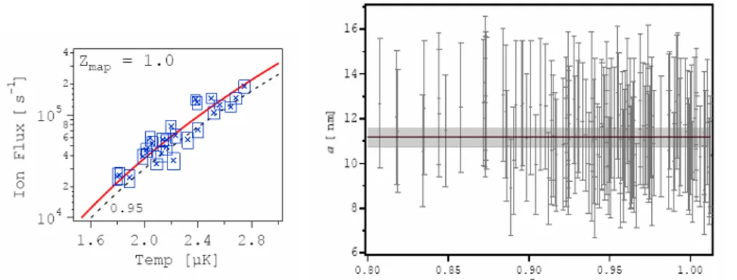
Fig. 3 –a) Signal d’ion en fonction de la temp´erature pour des nuages `a T = Tc. b)
les r´esultats finaux pour l’analyse des la d´etermination de la longueur de diffusion de l’He∗.
Choisir des donn´ees `a T = Tc a jou´e un rˆole tr`es important dans l’analyse
Cette longueur a ´et´e mesur´ee en comparant le flux d’ions, qui a une d´ e-pendance forte avec a, avec la densit´e atomique de nuages `a la temp´erature critique (voir Fig.3-a). Ceci a ´et´e fait en utilisant les m´ethodes d´ecrites ci-dessus pour l’analyse du tdv ainsi que du signal d’ions. Le r´esultat obtenu confirme une analyse pr´ec´edente et donne a = 11.2 nm. L’analyse statistique des r´esultats a donn´e un ´ecart type d’environ 0.3 nanom`etre (voir le Fig.3-b).
Outline.
In 1925, Albert Einstein predicted that if an ideal gas of bosonic atoms were cooled below a certain transition temperature it would undergo a phase transition to a new state where a macroscopic fraction of the atoms would occupy the same fundamental state of the system[1] creating a highly coher-ent atomic ensemble. As Einstein pointed out, this remarkable statemcoher-ent is a consequence of the statistics of identical particles with integral spin, which had been recently derived by himself and Satyendra Nath Bose[2]. De-spite this early prediction, it only became possible in the 1990’s to create a Bose-Einstein condensate (BEC ) in dilute atomic samples, as Einstein had originally imagined.
BEC in dilute gases.
In these experiments the gas is strongly localized in both coordinate and momentum spaces[3]. To avoid the formation of dimmers (and also to reduce losses due to inelastic collisions) the sample is very dilute, typically millions of times less dense than an ideal gas at atmospheric pressure and room temper-ature. This leads to extremely small phase transition critical temperatures, typically in the range of microkelvin1, and has long constituted a considerable
challenge for experimental physicists.
The first atomic BEC s were obtained in 1995. The impact was so great that only six years later E. A. Cornell, W. Ketterle and C. E. Wieman re-ceived the Nobel Prize in 2001 ”for the achievement of Bose-Einstein con-densation in dilute gases of alkali atoms, and for early fundamental studies of the properties of the condensates”. One remarkable experiment reported by Wolfgang Ketterle’s group at MIT demonstrated that when two indepen-dent BEC s were superimposed they interfere[5] in much the same way as coherent light. This was the first clear demonstration of first order coher-ence of the associated atomic quantum field, which could be characterized through the visibility of interference fringes. Other impressive experimental achievements were the realization of pulsed and CW atom lasers[6, 7, 8, 9] and the observation of the interference of two matter-wave beams emitted
1In condensed matter systems critical temperatures are much higher. For example, the superfluidity of liquid helium takes place at 2.18◦K[4].
from two spatially separated regions of the same BEC [10]. These pioneering experiments have verified that in many senses, below the BEC condensation threshold, bosonic atoms become coherent in phase and degenerate in energy, much like the stimulated emission of a single mode laser beam. The similar-ities between coherent atoms and photons[11] allow many of the key ideas of quantum optics to be directly carried over to describe coherent atom optics. However there are several key differences between atoms and photons; atoms have both mass and internal states that have no counterparts in photons. An especially important difference is that atoms can also interact directly with each other, without requiring a nonlinear medium that mediates the inter-action between photons. For example, it is possible to carry out an atomic four-wave mixing experiment in which three different coherent atomic beams interact in a vacuum to generate a fourth beam[12].
Bose-Einstein condensation in Metastable Helium.
To get to the point where it was possible to produce a BEC in a di-lute sample, many important new experimental techniques have contributed. Among these, the demonstration of optical trapping of macroscopic objects dates from the beginning of the 70’s[13] and of neutral atoms in the early 80’s[14, 15]. Optical cooling techniques [16, 17, 18] were developed soon after and also those for magnetically trap the atoms[19]. Evaporative cooling was developed initially within the efforts to achieve BEC in hydrogen, also in the early 80’s[20].
The first experiments achieving BEC were done in 1995 and counted three different alkalis: rubidium (87Rb)[21], sodium (23Na)[22] and lithium
(7Li)[23]. Still within the alkalis, there are today BEC experiments with
potassium (41K)[24], with another isotope of rubidium (85Rb)[25] and also with cesium(133Cs)[26], this one using an optical dipole trap[27]. Also
us-ing this type of trap, ytterbium (74Yb)[28] and chromium (52Cr) [29] have
recently attained condensation. The pioneering atom, hydrogen, was con-densed only in 1998[30].
In 2001, it was the time of metastable Helium (He∗) to join the group of condensed species in a dilute atomic sample[31, 32]. It was also the first time BEC was done in an atomic gas not in the electronic fundamental state2.
Unlike the alkali, in the He∗ experiment the atom is initially prepared into its first electronic excited state 23S
1, a metastable state with a life time of
9000 seconds and internal energy of 20 eV.
There are two main reasons for preparing the sample in the 23S
1 state.
First, unlike the ground state, this metastable state has a closed optical tran-sition to the excited triplet 23P2 state3, that can be addressed with available
2There is also one experiment aiming to achieve BEC with20Ne[33] and another where metastable xenon was optically trapped[34].
3The 23P
laser sources (at the wavelength 1083 nm). This is essential to optically trap and cool the sample[36, 37] and also to use the most standard optical detec-tion schemes as absorpdetec-tion, fluorescence and refractive measurements[38].
The sample is also prepared in the metastable state to have a perma-nent magnetic dipole moment, necessary for magnetic trapping. Moreover, the magnetic polarization of the sample strongly suppresses the inelastic col-lisions between He∗ atoms, increasing the stability and the lifetime of the sample[39]. This has motivated the design of our experiment, where He∗ was condensed for the first[31] and, also, in another experiment at the ´Ecole Nor-male Sup´erieure (ENS )[32], that has achieved BEC almost simultaneously as in our group. He∗ condensation was also be attained in Amsterdam[40] and, recently, also in Canberra[41]. The Amsterdam’s group has also achieved degeneracy in the fermionic isotope 3He using a two-color magneto-optical trap [42] and sympathetic cooling[43].
The He∗ unique diagnostic tools: I-single atom detection.
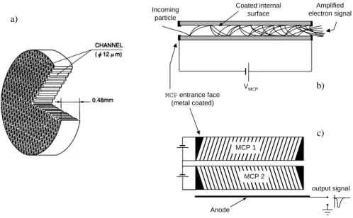
The internal energy of the He* is sufficient to extract an electron from a metallic plate. This is used in our experiment, as well as in the one at Amsterdam, to detect the atomic cloud with micro-channel plate (MCP)[44]. This device works as an electron multiplier and outputs a signal proportional to the atomic flux that arrives at its sensitive surface. The extremely good MCP time response and high gain allows single atom detection, which is very difficult to achieve in more conventional BEC experiments based upon optical imaging.
The use of a MCP along with a position sensitive detector based on a delay line has allowed us to make an intensity correlation experiment with massive particles, an experiment that is conceptually very similar to the one carried out in 1956 by Robert Hanbury Brown and Richard Twiss with thermal light.
This experiment remains nowadays as one of the landmark experiments in quantum optics. It measured, for the first time, the second order temporal coherence (i.e., the correlation function) of photons from a thermal field. We will refer to this experiment, form here on, as the HBT experiment. From a particle point of view it quantifies density correlations and is related to the conditional probability of finding one particle at a certain location given that another particle is present at some other location. Photons originating from a thermal source have the tendency to be detected close together, an effect usually referred as bosonic bunching. This behavior is common to any source of thermal bosons as is the case of a thermal cloud of He∗ atoms. The single atom detection capability of our experiment is particularly convenient for carrying out a HBT type of experiment with massive particles.
to 23S
The He∗ unique diagnostic tools: II - the ion signal.
BEC in spin polarized He∗ is possible because the inelastic collisions are highly suppressed. Even so, a small rate of ionizing processes remains giving rise to a small but still detectable flux of ions, proportional to the cloud’s density. This is a very remarkable tool that allows following the evolution of the cloud’s density toward BEC, passing through the phase transition, in real time and in a non invasive way. In particular, the ion signal can be used for determining when the critical phase transition happens. At this partic-ular instant of time, the cloud’s density and the ion flux increase abruptly, indicating the phase transition.
We have used the ion signal and its exceptional behavior close to the critical point to help producing clouds at the vicinity of the BEC threshold. This was used in one of the experiments we carried out, on the determination of the S-wave scattering length of the He∗, a (which we will refer in the following). The determination of the critical point through the ion signal analysis could also be used in several other experimental situations. For instance, it could be used to sort data in a HBT experiment with clouds at the critical temperature. This would allow the investigation of quantum bosonic effects and of critical fluctuations through the analysis of the density correlation function.
The experimental work realized during the thesis.
In this manuscript we describe and present the results of three different experiments realized during my thesis.
The one we describe first is the already referred HBT experiment that has measured the intensity correlation function of a falling He∗ cloud. In this ex-periment, we realized for the first time a measurement of a massive particles’ correlation function for a BEC and also for non-degenerate atomic samples at different temperatures close to the critical temperature. We have confirmed the expected behavior of the second order coherence function of bosons, with similar results as those already known for photons. This experiment is briefly described in Chapter 3, where we also show its main results.
The other two experiments realized during my thesis are quite different from the one just referred. They were carried out before the HBT experi-ment and had the goal of measuring collisional properties of the He∗: i) the ionizing rates due to inelastic collisions between two and three atoms of He∗, β and L respectively[45] and; ii) the He∗ S-wave scattering length a[46], the fundamental parameter that characterizes elastic collisions between atoms in a very cold gas. Conceptually, both experiments rely on a comparison be-tween the ion flux produced within the cloud and its mean density, inferred from the analysis of the atomic time of flight (TOF ) that is recorded when the cloud is released from the trap and falls over the MCP. In the first experi-ment (on the ionization constants), this comparison was done for condensed
clouds whereas in the second, we used thermal clouds close to the critical temperature.
We have summarized the description of the experiment on the measure of β and L to the Appendix B, where we also show its main results. The theoretical description of the BEC and of its time of flight is also postponed to the Appendix A.
The results obtained in this experiment for β and L were used subse-quently in the data analysis of the experiment for measuring a. This latter one is described in detail in Chapter 5. As we referred above, it relies on the comparison of the ion flux of clouds at the critical temperature, which varies considerably with a, with the corresponding atomic densities, only weekly dependent on a. We use this experiment and its data analysis to describe, in Chapter 4, a few techniques we developed during the thesis to analyze both the ion flux and the atomic TOF of thermal clouds at the critical point. In Chapter 5, we discuss their use for improving the accuracy on the cloud’s thermometry, mainly in the determination of the cloud’s chemical potential. We show that the reduction of the uncertainty on the determination of this quantity leads to a reduction of the statistical uncertainty in the final result of a.
Thermometry in the critical phase transition I: the ion signal analysis.
Along with the theoretical description of the intensity correlation func-tion, the development of techniques of analysis of the ion signal and of the atomic TOF has constituted the ”tour de force” of the work I did outside the laboratory during my thesis.
To be able of carrying out any sort of experiments with atomic clouds at the critical phase transition, one needs first to have a very reproducible process to produce such clouds. In Chapter 4, we show that this is not possible due to the bias field fluctuations of the trapping potential: the shot-to-shot variation of the bias field makes that, even for similar conditions for the evaporative cooling and similar loads of the magnetic trap, the resulting clouds vary considerably in number of atoms and temperature.
A way around this is to take data as close as possible to the critical tem-perature and then use some process to sort from these data set those that better correspond to clouds at T = Tc. To get as close as possible to Tc
may be achieved just by analyzing the ion signal which has the advantage of giving a real-time diagnostic of the cloud’s evolution. The phase transition imposes an abrupt variation of the density, which produces a rather spectac-ular increase of the ion flux signal. Somewhere within this transient period of time lays the critical point and, to get clouds at Tc, the evaporative cooling
should stop at that very especial critical time. The remaining question is how to determine accurately this critical time. If the scattering length and
the ionizing rate constants are known, the ion flux signal can be computed, taking some adequate model (with more or fewer approximations) for the theoretical description of the cloud’s density. In any case, this latter one has only two parameters: the cloud’s temperature and chemical potential µ (or, alternatively, the number of atoms). During evaporation, while the cloud cools down it also looses atoms due to the evaporation itself and also to the inelastic collisions. This leads to a continuous setting of the cloud’s chemical potential that ends, hopefully, with µ ≈ 0 and a BEC growing within the cloud. The analytical description of this process is hard to workout due to the mutual interdependence of the various processes involved4 making the
theoretical prediction for the time evolution of the cloud’s density and the ion flux a non trivial task.
In this thesis we have opted to carry out instead a simple numerical time-stepped simulation that computes the cloud’s density and chemical potential evolution, admitting a certain variation of the temperature imposed by the evaporation process. In this routine we use a so called semi-ideal[47] model to describe the thermal cloud, which accounts to the BEC repulsion, with this latter described in the Thomas-Fermi approximation. Within the validity of this model, the routine is used to derive the location, on the ion signal, of the critical point.
The results of this simulation were used to characterize in a very generic way where the critical point should be found. This was used to deal with real data and to compute an empirical curve expressing the expected ion flux generated by a cloud at the critical point in function of the corresponding instant of time it happens, for all attainable critical temperatures in our experimental conditions (see §4.2.4). This critical curve was used to guide the procedure of taking data (it indicated where the evaporation should stop) and also in the posterior procedure to sort the data.
Thermometry in the critical phase transition II: The time of flight signal.
The determination of critical point through the analysis of ion signals can be made very accurate but only if the bias field fluctuations are small. Unfortunately, this is not the case in our setup and the precise moment at which the cloud is at T=Tc changes from one experimental run to the next. We show in Chapter 4 that this leads to an uncertainty in the determination of the cloud’s chemical potential of about 10% of kBT , which is not entirely
adequate for sorting data at Tc.
This task should be carried out through the analysis of the cloud’s time of flight (TOF ) signal that is a direct inspection of the cloud’s density (after
4This is true even for the simplest case where the thermal and the condensed clouds are treated as separate objects, using semi-classical formulae for describing their density profiles and mean field models for the interatomic interactions.
expansion). This is done fitting the TOF s to a theoretical model. Here, as before, the main problem is to obtain an accurate determination of the cloud’s chemical potential. There is no simple fitting model that describes the cloud’s density in both sides of the critical transition: the fitting expressions used for thermal clouds are not defined for positive chemical potentials. Therefore, for TOF s where this quantity is identically zero, a standard fitting procedure is unable to work properly since it cannot compute the chi-square in both sides of that minimum. In chapter 4 we propose a strategy (further detailed in Appendix D) to go around this problem. The idea, in brief, is to extrapolate the behavior of the chi-square for µ < 0 into the critical region, where µ ≈ 0, and thus avoiding the computation of this quantity for µ > 0. The resulting uncertainty in the value found for the chemical potential is estimated in Appendix D to be of about 2.5% of kBT . We will denote this procedure in
the following as the χ2-map strategy.
The characterization of the noise in the experimental TOF and the use of an appropriate model for fitting these signals are essential ingredients to reduce the uncertainty on the determination of µ. One has two different issues: the description of the cloud’s density at thermal equilibrium inside the trap and the description of its expansion under the influence of gravity.
The standard formulae for the description of density of harmonically trapped gases are derived in the semi-classical approximation and are ex-pressed using infinite sum functions known as Bose functions (which are easily computable). These expressions may include a first order correction, on the trapping frequency, to account for the finite size of the cloud. This is however the only corrective term that can be considered, since all other higher order terms leads to diverging infinite sums. This leads us to further investigate the validity of the semi-classical approximation when used in the description of the cloud’s density. We found that, when the contribution of the fundamental state is taken into account, the peak density critical value should be around 6.24/λ3
T instead of the usual ζ(3/2)/λ3T, with λT the
ther-mal de Broglie wavelength. The discrepancy between an exact calculation and the semi-classical expressions is however only important close to the cen-ter of the cloud. We show that a single integration of the atomic flux over a spatial direction is enough to make the semi-classical approximation valid. We have verified in Chapter 2 that, for our data analysis, the semi-classical expression gives a good enough description of the atomic TOF signal. In Chapter 4 we complement this simple model for the ideal gas by including interatomic interactions. This is done within a mean field model[48] that relies upon some approximations of which the validity will be discussed.
The formalism for treating the expansion and fall of the cloud is given in Chapter 2, for the ideal gas case. We use a Green function to propagate the harmonic oscillator wave functions in the gravitational field and, using a
quantum mechanic definition of the matter flux, compute the atomic TOF. As for the cloud’s density, the influence of the interaction between atoms is left to Chapter 4, where we discuss the hydrodynamical regime.
The second order coherence function in an atomic beam.
The formalism needed to derive the atomic TOF is extended in Chapter 3 to deal with the intensity correlation function of the particles flux when the cloud is released from the trap. This theoretical analysis has derived typical values for the transverse and longitudinal atomic coherence length that have confirmed the possibility of performing an HBT experiment with our apparatus. It has also helped in the study of the necessary upgrades of the detection system. We will briefly discuss these upgrades[49] and show the main results of this experiment[50].
The data treatment on the scattering length experiment. The systematic error on the determination of a.
Despite all our efforts to have a proper cloud’s thermometry and an ac-curate determination of a, the value we have measured is affected by a large systematic error. Chapter 5 starts by describing our first data analysis on this experiment. It is based on a model that assumes from the beginning that µ = 0, avoiding the determination of the actual value of the chemical potential for each cloud[51]. We develop then a second approach, using the χ2-map strategy to determine the chemical potential of each individual cloud and use that value in the determination of a. This second analysis conduced to a smaller statistical uncertainty on the value we find for a, which how-ever is not very different form the one that had been obtained previously: a = 11.2 ± 0.4 nm.
A recent and very precise light-induced collision spectroscopy experiment, made in the group at the ENS has rather obtained a = 7.512 ± 0.005 nm, a result that indicates we have committed an error of about 50% in our experiment. This manuscript ends with an attempt to explain this huge discrepancy. We will address the description of the process through which the cloud is released from the trap. We show that if the trapping potential switch-off is not fast enough, the initial moments of the cloud expansion may change dramatically the thermometric interpretation of the cloud’s TOF, both for thermal and condensed clouds.
The plan of the manuscript.
In the following we present the outline of the thesis, highlighting for each Chapter, the more pertinent aspects regarding the structure of the manu-script.
• Chapter 1 - In the first Chapter we present a detailed description of our experiment in what concerns the production and detection of an ultra-cold could of He∗. Most of the first and second Sections of this
Chapter describe very standard techniques widely used in the exper-imental field of cold quantum gases. We also introduce the working principle of the MCP (§ 1.3.1) and the process through which the cloud is released from the trapping potential. This Chapter discusses finally the two major experimental difficulties we have to deal with in our setup. The first of these, referred above, is bias field fluctuations. Sec-tion §1.2.2 describes in some detail this problem. The second major experimental problem we faced in this thesis had to do with the im-possibility of getting an absolute calibration of the number of atoms in the atomic time-of-flight signals (see §1.3.6.1).
• Chapter 2 - This Chapter introduces the theoretical models and defini-tions used throughout the manuscript. It is divided into two Secdefini-tions: i) the theoretical description of an ideal gas in thermal equilibrium inside a harmonic potential (§2.1.1); ii) the description of the atomic time-of-flight in the ballistic approximation (§2.2). In i) we discuss the criteria for defining the critical phase transition (§2.1.1.1), in particular for the cloud’s peak density and the validity of the semi-classical approxima-tions (§2.1.1.2). In paragraph §2.2.2, we introduce the approximaapproxima-tions we use in the analysis of the atomic time-of-flight signals.
• Chapter 3 - This Chapter is based on Ref.[52] and details the calcu-lation of the intensity correcalcu-lation function in the atomic flux generated by the free fall of a cloud of atoms in the ideal gas approximation. The results reported here gave the first indication that our setup could be used in HBT experiment. The Chapter starts by reviewing the main ideas of first and second order coherence theory in optics and its generalization for a quantum field of massive particles. This is done explicitly for an ideal gas trapped in a harmonic trap (§3.3), stressing particularly the case of a cloud at the critical temperature. The case of an expanding cloud under the effect of gravity (§3.4) is then dealt with and expressions for the intensity correlation function are derived. The last Section of this Chapter reports briefly on the upgrade of the setup and on the main results of this experiment.
• Chapter 4 - In this Chapter we describe the techniques we have devel-oped during the thesis for the cloud’s thermometry within the analysis of both the ion flux (§4.2) and the atomic TOF signals (§4.3). The first Section of this Chapter deals with the problem of how to interpret the ion signal. We start by presenting the simple model used in the simu-lation of the cloud’s density and the ion signal temporal evolution. We discuss two possible procedures to determine the critical point in an ion signal and present the critical curve obtain for real data. We also derive
the relation between the experimentally observed bias field fluctuation and the uncertainty on the determination of the chemical potential. The second part of this chapter describes the mean field model used for fitting the TOF signals and the correction on the obtained temperature due to the hydrodynamical effect.
• Chapter 5 - This manuscript last Chapter makes use of the cloud’s thermometry to measure the scattering length. We start by describ-ing this experiment in some details (§5.2) and the procedure we used, initially, to analyze the data. Then, and after discussing the data dis-persion we observe on the result we explain how we can improve the accuracy, by improving the thermometry of the acquired TOFs. The proper determination of the temperature and fugacity of a thermal cloud at the vicinity of the critical point is the goal of the χ2-map
tech-nique, a method we introduce in this Chapter. The last Section of this manuscript discusses the error committed on the determination of a.
Bose-Einstein Condensation of
Metastable Helium: the
apparatus.
In this Chapter we will present our He∗ experiment. In the first part we will describe how we produce a cloud of cold atoms of He∗and how we manage to achieve BEC with it; in the second part we describe how we detect the atomic cloud.
All the methods we describe here to trap and cool down the atoms are standard techniques in most of BEC experiments in dilute atomic samples. We will start the description of our experiment by presenting the magnetic trapping and the evaporative cooling techniques, explaining how they work and also describing their experimental implementation in our setup. The combination of these two techniques has constituted the final breakthrough in the achievement of Bose-Einstein condensation in dilute atomic samples. The evaporative cooling is just the final part of all the processes involved in the production of a BEC and, in our experiment, it takes about thirty seconds to be completed. Most of the work presented in this thesis is related with the physics of non-degenerated clouds near the critical transition point. Since this transition is attained in the last few seconds of the evaporative cooling, this process takes an important role in many of the subjects presented throughout this manuscript.
To get a magnetically trapped atomic cloud, many other steps must be taken however. In the paragraph §1.2.3, we will come back a few steps back in the experimental track to explain how we manage to produce the He∗ atoms (the atomic source) and also to describe all the necessary laser based techniques we use to achieve loading an already cold atomic cloud into the magnetic trap.
Diversely to the techniques we use to trap and cool down the atoms, the detection system in our experiment can not be considered as a standard one when compared with most of the cold atoms experiments. Rather than using optical methods (like imaging the cloud’s absorption of a laser beam), in our experiment the atoms’ detection is made electronically using a micro-channel plate (MCP). The use of the MCP in this case is possible due to the He∗ internal
energy, sufficient to extract an electron from the metallic frontend surface of the MCP. We show how we use this device to detect our cloud. With it, it is even possible to make single atom detection. This is a very important ability of our setup and we will show in Chapter 3 how it was used to measure the density-density correlation function. Before entering into the experiment description, we will briefly present the road map we need to follow, in the experimental point of view, to achieve condensation.
1.1
Road map to achieve BEC in He
∗.
The critical phase transition.
Traditionally, the critical transition to BEC is presented for the homogeneous ideal gas case. In this case, BEC occurs when the spatial atomic density, n, and the gas temperature, T , is such that the following relation is respected[3], n × λ3T = ζ (3/2) , (1.1) where T enters in the definition of λT =
q
2π~2
M kBT, the de Broglie thermal
wave length with M the atomic mass. In practice, the atomic cloud has to be trapped somehow and its density is, in general, inhomogeneous. This is the case of a harmonically trapped cloud, for which the above relation is still valid if one replaces the homogeneous density by the cloud’s peak density, n(0), the density at the center of the trap. The factor n(0) × λ3
T is, in fact,
the phase space density and, its critical value ζ(3/2) ≡ 2.612 is the objective one pursuit for achieving BEC.
λT λT
n-1/3
n-1/3
Figure 1.1: An intuitive interpretation of the critical phase transition relation for a dilute cloud of cold atoms. Here, λT is the de Broglie thermal wavelength of the
atoms and n, the cloud’s density. When λT ∼ n−1/3 the atoms start overlapping
and the phase transition occurs.
A generally used interpretation of the expression in Eq.1.1 is the one sketched in Fig.1.1: for low enough temperatures, the atoms wave functions start to spread out and then to overlap with theirs neighbors, becoming indis-cernible. In here, the critical transition happens when the spatial separation between two particles is comparable to the de Broglie thermal wavelength of their wave packets, a similar relation as that stated in Eq.1.1. We will revisit this relation in the Chapter 2, in more detail.
In cold atoms experiments, the typical value for the critical temperature is around 1µK, several orders of magnitude smaller than, for example, the critical temperature for the lambda transition point where the liquid helium becomes superfluid, around 2.2K[4]. Note that, for a critical temperature of 1µK, the relation of Eq.1.1 predicts a critical density for the He∗ gas around 1012cm−3, which is seven orders of magnitude smaller than the air density at
Brief comment in all-optical atom cooling methods.
Up to the moment this manuscript was finished, all BEC experiments have only attained condensation trough evaporative cooling methods, either in magnetic or dipole optical traps. As we will further explain in §1.2.1.3, one of the main disadvantages of the evaporative cooling is to be a depletive method: to cool down the cloud, some atoms (the hottest) has to be expelled out of the trap. In fact, due the finite life time of the sample, typically a few tens of seconds, evaporation must be completed in a time that must be short when compared to the trap losses rate. Speeding up the evaporation implies increasing the number of ejected atoms and, in the end of the cooling process, only a small percentage of the initial population remains trapped and cooled down to the BEC transition temperature.
There are also atom cooling techniques that work by laser cooling alone. There are especially two techniques that allow attaining temperatures below the recoil limit, kBTr = (~k)2/2M 1: the velocity-selective coherent
popu-lation trapping (VSCPT) [53, 54] and the Raman cooling [55, 56]. These methods relies on the existence of single atom dark states, a Raman induced coherent superposition of two states with momentum ±k, insensitive to the cooling laser. These are stationary states, eigenvectors of the total Hamil-tonian, being populated by atoms coming from the absorbing states through momentum redistribution due to spontaneous emission. The attained tem-peratures are in the nanoKelvin regime and, unlike the evaporative cooling, they preserve the initial number of atoms. Moreover, these all optical meth-ods may complete an entire cooling cycle in a fraction of a second. This is an important advantage when compared to the tens of seconds needed by the evaporative cooling stage 2. Additionally, laser cooling methods may
be used to cool fermionic samples down to the superfluid BCS state[57], a regime where evaporative cooling techniques are unable to attain[58].
Unfortunately, laser cooling techniques present still serious limitations to achieve large atomic densities. In here, light reabsorption appears as the main obstacle for achieving low temperatures at the very dense optical media of the cold gases close to the critical transition. The above referred velocity depen-dent dark states are dark only for laser light involved in the cooling scheme. These atoms can interact with the light emitted spontaneously by other atoms in the sample, making them abandon the absorption-free state[59]. Several strategies have been proposed to overcome this difficulty as, for example, using very anisotropic potentials, where most of the spontaneously emitted
1This temperature corresponds to the kinetic energy that is transferred to the atom when it spontaneously emits a photon with momentum ~k.
2These times are reduced several times for experiments done in microchips devices, where the higher confinement of the atomic cloud enhances the elastic collisions rate (see also §1.2.1.3).
photons does not interact with the atomic sample, or very confining traps with linear sizes comparable to the wavelength of the emitted photon. The most promising however is a scheme known as the festina lente scenario[60]. Here, the time between two spontaneously emitted photons, Γ−1, controlled by the Raman pumping rate, is made to be much larger than the inverse trapping frequency time. Theoretical predictions show that, within this con-dition, reabsorption processes are suppressed, avoiding the heating of the atomic sample. Even so, up to this date there is no experimental prove of the usefulness of any of these schemes for cooling atomic samples down to the degeneracy point.
Road map to the BEC.
Despite its depletive character, with evaporative cooling it is possible to increase the atom’s phase space density up to the critical BEC transition. As we will describe in the following Sections, in our experiment, this technique is used on an atomic cloud trapped in a magnetic trap. The task of capturing and pre-cooling the atoms before loading them into the magnetic trap is taken by a magneto-optical trap (MOT). This apparatus uses both laser beams and magnetic fields to confined and cool down the atoms. The MOT is loaded by an atomic beam delivered by a hot atomic source. To achieve loading the MOT, a few other laser based techniques are used to first collimate transversely and then reduce the longitudinal velocity of the atomic beam (see §1.2.3).
In the Table1.1 we make a summary of the three intermediary stages needed to attain BEC in our experiment. There we present typical values for the phase space density, the number of trapped atoms and the cloud’s temperature and density.
1.2
Producing a metastable helium Bose
Ein-stein condensate.
Metastable helium has two fundamental characteristics that allow achieving BEC. First, the He∗ atom can be optically manipulated by commercial lasers in the closed optical transition between the 23S
1 and 23P2 states; second, it
has a permanent dipole moment, µ, which allows using a magnetic trap. We will come to both of these characteristics in the following Sections. We start now with the latest and explain the magnetic trapping of neutral atoms.
1.2.1
The magnetic trap and evaporative cooling.
The magnetic trap and the evaporative cooling process rely in very simple but powerful ideas. Here, we revise briefly those ideas and emphasize the
n0λ3T N T [µK] n0 [cm−3] Atomic beam 10−30− 10−20 − − − Laser trapping and cooling 10 −6 108 102− 103 109
Magnetic trap and
evaporative cooling ≈ 1 10
3− 106 0.1 − 5 1013
Table 1.1: The cloud’s degeneracy parameter, number of atoms, temperature and density at the end of each of the three main techniques involved in the BEC pro-duction: the production of a atomic source, the trapping and pre-cooling with laser based techniques and, finally, the evaporative cooling of the magnetically trapped cloud down to the BEC transition point.
most important details with respect to our experiment.
1.2.1.1 Trapping neutral atoms with a magnetic field.
Unlike the alkalis, the helium in its fundamental state is a singlet state with-out dipole moment. However, exciting one of its electrons to the first elec-tronic excited state 23S
1, it stays in a metastable state (with a life time bigger
than 2 hours [61, 62]) which has a permanent magnetic dipole moment, µ. Immersed in a magnetic field, the He∗ atom dipole has a position depen-dent interaction energy given by
U (r) = −µ · B(r).
In the classical picture, the magnetic dipole experiences a torque due to the interaction and processes around the magnetic field B at the Larmor pre-cession frequency, νL = |µB|/~. If this frequency is much larger than the
inverse of the typical variation time scale of the magnetic field, the dipole µ will adiabatically follow the magnetic field B. This adiabatic condition, if re-spected, predicts that the atom will preserve all the time its initial magnetic spin polarization. We will see further on in this Section that the magnetic field in our trap is never smaller than 0.3G. To this field corresponds a Larmor frequency of about 106Hz, which is about three orders of magnitude bigger
than the maximum oscillation frequency of the trap. The adiabatic condition is then fulfilled and we may replace the scalar product of the above equa-tion by U (r) = gJµBmJ|B(r)| with mJ the projection of the total angular
Thus, to trap the atoms, the potential U (r) must have a local minimum at some given location and deep enough when compared with the atom’s thermal energy kBT .
It is a well known result that the Maxwell equations predict the non existence of local maxima of dc magnetic fields in free space[63]. Thus, the only way to get a minimum in the potential energy is to create a minimum in the magnetic field with also gJmJ > 0. This is the case of the magnetic
sub-level mJ = 1 of the electronic state 23S1. Since for this state L = 0, J ≡ S
and gJ = +2. An atom polarized in this state is then a low field seeker in the
sense that it tends to minimize the interaction energy moving into the field minimum. The electronic state 23S
1 has also other two magnetic sub-levels
with projections mJ = 0 and mJ = −1. An atom polarized in this latter one
simply fly away from the minimum of the magnetic field, escaping the trap. However, if it is polarized in the mJ = 0 sub-level, the atom is insensitive to
the magnetic filed and will simply fall under the effect of gravity.
B µ J mJ=+1 U(r) r mJ=+1 mJ=0 mJ=-1 µ B
Figure 1.2: The left hand side image illustrates the precession of the pure spin state mJ = 1 around the magnetic field. The right hand side sketch represents
the equipotential curves corresponding to the three magnetic sub-levels of the electronic state 23S1 deformed by the Zeeman effect induced by a parabolically
varying magnetic field. In here, the low field seeker state is the one with mJ = +1,
corresponding to a magnetic moment µ = −gJµ~BJ, antiparallel to the direction
of the field. The sub-level mJ = 0 is insensitive to the magnetic field and the one
with mJ = −1 is an anti-trapping state. Atoms polarized in one of these two states
escape from the trap.
In order to verify the previously referred adiabaticity condition and pre-serve the atom’s spin polarization, the trapping potential needs to have a finite minimum. If an atom passes, momentarily, through a zero magnetic field it looses its magnetic quantization axis and may spin flip into any of the magnetic sub-levels. If it flips to a non-trapping state, it is lost from the trap. To avoid this effect, known as Majorana losses, it suffices then that the trapping potential is always non null. However undesirable when