Maintenance Policies

HAL Id: hal-01007539

https://hal.archives-ouvertes.fr/hal-01007539

Submitted on 16 Jun 2014

HAL is a multi-disciplinary open access archive for the deposit and dissemination of sci-entific research documents, whether they are pub-lished or not. The documents may come from teaching and research institutions in France or abroad, or from public or private research centers.

L’archive ouverte pluridisciplinaire HAL, est destinée au dépôt et à la diffusion de documents scientifiques de niveau recherche, publiés ou non, émanant des établissements d’enseignement et de recherche français ou étrangers, des laboratoires publics ou privés.

Maintenance Policies

Alaa Chateauneuf, Franck Schoefs, Bruno Capra

To cite this version:

Alaa Chateauneuf, Franck Schoefs, Bruno Capra. Maintenance Policies. Construction Reliability: Safety, Variability and Sustainability, pp.253-270, 2012, �10.1002/9781118601099.ch13�. �hal-01007539�

Maintenance Policies

13.1. Maintenance

Maintenance can be defined as the combination of operations allowing the system being considered to be maintained in a desired state of performance. The possible operations include inspections, repairs and replacements. This chapter defines various types of maintenance, as well as some definitions related to structural lifetime, T. Remember that the failure probability is denoted as Pf and reliability by R = 1-Pf. The failure rate, given as λ(t), and measured at time t, can be simply defined as the number of failed items per unit time. Readers can refer to a number of works [LAN 05], [MOR 01], [NAK 02] for more details concerning the concepts related to the evaluation and management of ageing industrial systems, in a wider scope than just for construction.

13.1.1. Lifetime distribution

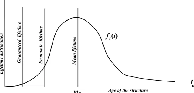
Distribution of lifetime T, denoted fT, can be estimated either by a physics approach or by statistical approaches. For most industrial systems, the specification of “mean lifetime” mT does not present a useful indicator (Figure 13.1), as a very high failure probability leads to undesired consequences in terms of economic and life losses. By contrast, the specification of “guaranteed lifetime”, corresponding to very low failure rate, implies the under use and underating of a system, and consequently leads to economic losses that could be avoided. We can therefore define the “technical–economic lifetime” as the service time behind which either the

industrial risk is considered very high, or required additional investments cannot be refunded during the system’s future life. An optimal compromise can be found on the basis of this technical–economic lifetime, corresponding to the minimum expected total cost. This solution can be obtained by optimal balancing of initial and additional investments, risk of losses and costs of monitoring and maintenance actions.

Figure 13.1. Lifetime distribution

13.1.2. Maintenance cycle

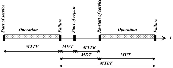
At the beginning of a service life, a structure is in a state of good operation until the occurrence of its first failure (Figure 13.2). In many cases, a system is partially or totally repairable (or replaceable) and can re-start a new life-cycle until the next failure. The consideration of failure in service is generally accompanied by some administrative and technical delay which should be taken into account before starting effective repair operations which themselves require a specific time interval. Knowing that uncertainties cannot be avoided, the duration corresponding to each state is intrinsically random and, consequently, we should not only consider the mean values but also the associated dispersions. Figure 13.2 illustrates the evolution of a system in service, and we can distinguish the following periods:

– Mean Time To (first) Failure (MTTF): corresponding to the expected time for the occurrence of the first failure after the beginning of the system’s operation. For unrepairable systems, the MTTF corresponds to the expected lifetime;

– Mean Time Between Failures (MTBF): corresponding to the expected time between two successive failures of the same component/structure, including the down time during maintenance (i.e. this time is defined by the interval between the

f

_T

(t)

t

G u ar an te ed l ifet ime m_T Me an li fet ime E co n om ic li fe ti m e

Age of the structure

L if et im e di st rib ution

moments of the occurrence of successive failures). The MTBF is divided into an operation period, known as the Mean Up Time (MUT), and a non-operating period, known as Mean Down Time (MDT);

– Mean Up Time (MUT): corresponding to the expected operation time from the end of repair till the next failure;

– Mean Down Time (MDT): corresponding to the expected time during which the system is stopped, from the occurrence of failure till the effective re-start of operation after repair. MDT itself can be divided into two parts: Mean Waiting Time (MWT) and Mean Time To Repair (MTTR);

– Mean Waiting Time (MWT): corresponding to the lapse of time before discovering the failure, for administrative procedures and for waiting for ordered or transported spare parts;

– Mean Time To Repair (MTTR): corresponding to the time necessary to carry out the repair operation, after having the material and human resources, until the total recovery of the service.

Figure 13.2. Maintenance cycle for repairable systems

13.1.3. Maintenance planning

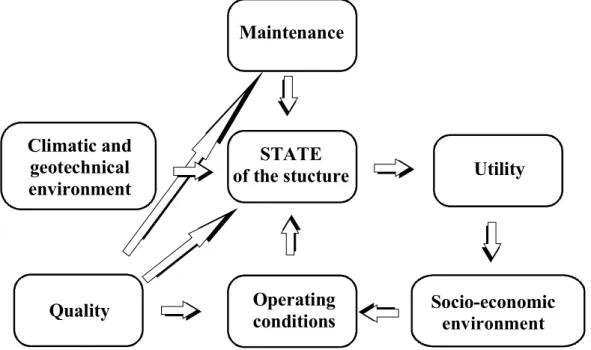
The utility of a structure depends on its capability to ensure good operation on one hand, and the socio-economic conditions, on the other hand. The capability of ensuring good operation is generally sensitive to the use conditions, the environment (especially climatic and geotechnical), the quality applied (materials, methods of analysis, transport or construction, etc.) and the procedures of maintenance and inspection. The use conditions are often affected by climatic, geotechnical and socio-economic environment. The maintenance itself is affected by the environment and by the applied quality (Figure 13.3).

t MTTF MTBF MWT _MTTR MUT MDT Operation _Fail u re St ar t of s erv ice St ar t of r epa ir Operation R e-s ta rt o f s erv ic e Fail u re

Figure 13.3. Inter-dependence of the conditions defining a structure’s utility

Maintenance planning should be based on equilibrated combination of preventive and corrective operations, in coherence with inspection results. The maintenance policy provides the sequence of decisions at various stages of the structure’s life. At the design stage, the maintenance parameters should be defined in an optimal way. At the operation stage, the designer and the user/owner should specify the inspections and actions in order to allow for better knowledge and management of the structure’s lifetime and performance (Figure 13.4).

Figure 13.4. Decision tree for inspections

The inspection parameters are the time span between successive inspections on one hand, and the depth of those inspections on the other hand. The inspection depth depends on the methods to be applied and their quality (i.e. technique, operator qualifications, etc.). The inspection results should lead to enough information to allow a decision to be made, with more or less precision, about whether maintenance

Maintenance

Climatic and geotechnical environment

STATE

of the stucture Utility

Socio-economic

environment

Operating conditions Quality

actions should or should not be performed. The main objective in this tree consists of minimizing the maintenance cost1, by taking into account safety constraints, and respect of standards, codes and regulations, without forgetting the limits of the available budget.

Therefore, the objective of a maintenance policy is to maintain the structure in a state of “good operation”. The aim is to keep “the observed reliability during operation”, called “operational reliability”, higher than the “target reliability”, called “intrinsic reliability”. This reliability-based maintenance policy consists of defining the tasks related to the following aspects:

– failure modes; – failure causes; – detection tools; – maintenance tools;

– procedures, methods and systems provided to realize maintenance;

– quantities (in terms of the outcome of maintenance and inspections), as well as the corresponding decisions.

13.2. Types of maintenance

Various classifications of maintenance action appear in the literature. According to Figure 13.5, the maintenance can be either preventive or corrective. Preventive maintenance can be either systematic, according to a time schedule defined in advance, or conditional, continuous or on request, or scheduled as a function of the information collected during the service life. At the same time, corrective maintenance can be either delayed, if the system can operate without risk until the scheduled time, or performed urgently, when repair is necessary to ensure safety and good operation.

13.2.1. Choice of the maintenance policy

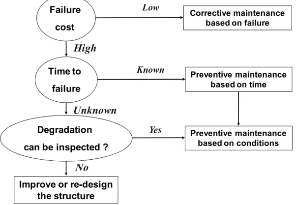
The choice of a maintenance policy depends on at least three criteria: (i) the impact of maintenance on the requirements of safety, availability and cost; (ii) the data characterizing the degradation; and (iii) the quality of performed inspections. When the impact of preventive maintenance is low, we prefer to wait until failure; corrective maintenance must be adopted for failed components (Figure 13.6).

1 The terminology of optimization under maintenance constraint (i.e. minimization of the expected total cost or maximization of expected utility) will be specified in Chapter 14.

However, if the failure cost is high, then preventive maintenance becomes necessary. If the mean time to failure can be estimated, verified or checked, preventive maintenance can be planned at regular time intervals (whether calendar time, real operation time, or any other specific time function).

Figure 13.5. Classification of various types of maintenance [CEN 01]

If the degradation can be inspected or monitored, preventive maintenance should be based on the knowledge of the real state of the system. However, in some cases, the programming of maintenance is not possible, due to large uncertainties regarding failure rates. We may face this situation when the induced failure cost is very high although the state of the system cannot be inspected, or when the failures are recurrent with low costs. In this latter case, the system should be re-designed in order to ensure appropriate robustness.

In addition to safety obligations, which are often mandatory and dominant, preventive maintenance is justified by the economic consequences when the following two conditions are satisfied:

– the preventive operations, or inspections, planned at fixed dates, cost globally less than the inevitable random corrective operation that could sometimes be performed at critical moments;

– the failure rate of the system for which we intend to apply a program of preventive maintenance, increases due to degradation of the components of the system with an increase in financial consequences.

In continuous production sectors, such as energy production plants and petrochemical plants, economic dependence is a result of production losses when the system is down, during corrective or preventive maintenance. In the case of

Maintenance

Preventive maintenance Corrective maintenance

Conditional maintenance Systematic maintenance Scheduled, continuous or upon request According

corrective downtime, additional costs have to be supported to take into account the direct and indirect consequences of failure (i.e. delay, de-damaging, urgent operation, etc.). During preventive or corrective operations, maintenance allows either the complete restoration of the components concerned or just the repair of the failure, with or without modifications of the ageing mechanisms. During corrective maintenance of a component, it is possible to take the opportunity of replacing other components of the same system preventively; in that case, we talk about “opportunistic maintenance”.

Finally, maintenance actions remain possible right until the stage of high degradation, whether this involves regular inspections of a system to know its state and the quality of its previous maintenance, in order to decide about the correction to perform on the observed damage, or what to repair in order to bring the system back to a state close to its initial state, or, ultimately, the replacement of components when they reach a state of technical obsolescence.

Figure 13.6. Flowchart of the choice of maintenance policy

These actions satisfy the economic requirements which should be taken into account in the development of the most recent theory of decision. The risk associated with each degradation and failure mode, has to be probabilistically evaluated. Possible actions like Risk-Based Inspection (RBI) [FAB 02a], Reliability-Based Maintenance (RBM), and Reliability-Centered Maintenance (RCM), repair or decommissioning have to be considered with their related uncertainties and possible consequences (i.e. economic losses, human fatalities, social impact, etc.), in order to

Preventive maintenance based on conditions Improve or re-design the structure Preventive maintenance based on time Corrective maintenance based on failure Failure cost Degradation can be inspected ? Time to failure Low High Known Unknown Yes No

determine the best possible decisions concerning the type of actions, including renovation and recertification of the inspected structure.

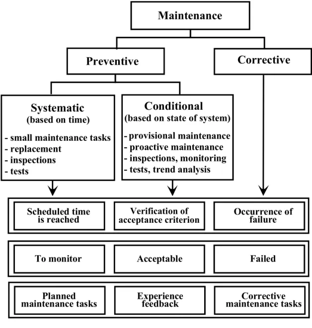
13.2.2. Maintenance program

A maintenance program consists of actions performed preventively (systematic or conditional) or correctively [ZWI 96]. Although systematic maintenance is performed at pre-defined times, conditional maintenance is performed when the acceptance criterion is reached, and corrective maintenance is performed urgently when failure occurs. Observations and inspection results lead to identification of the following states: acceptable operation, system to be monitored, or failed system. On the basis of the available information, (inspection results, experience feedback, expert opinion, etc.), the possible decisions concern the programming of alternatives (i.e. tasks of preventive and corrective maintenance) are made.

Figure 13.7. Flowchart of maintenance program

Maintenance

Preventive

Corrective

Scheduled time

is reached acceptance criterionVerififcation of Occurrence of failure

Systematic

(based on time) - small maintenance tasks - replacement

- inspections - tests

Conditional

(based on the state) - previsional maintenance - proactive maintenance - inspections, monitoring - tests, trend analysis

To monitor Acceptable Failed

Planned

maintenance tasks Experience feedback maintenance tasksCorrective (based on state of system)

provisional

Verification of acceptance criterion

13.2.3. Inspection program

An inspection program starts by defining the system and the performance criteria (Figure 13.8); this step implies the collection of data concerning the system and its environment. A Qualitative Risk Analysis (QRA) is therefore performed to determine the failure modes, as well as their causes and consequences (using, for example, RAMS methods, as described in Part One). In this step, the logical representation of the system must be established, in order to define the required functions and the interactions between components and sub-systems. The next step consists of estimating the failure rates and consequences, in order to allow for ranking according to risk levels.

Figure 13.8. Flowchart of an inspection plan. (“Defining the possible damage” implies the definition of degradation mechanisms; counting failures and degradations

is usually sufficient, compared to evaluation of the failure rate)

Inspection program

Define the possible damage

Define the possible inspections of each damage Estimate the reliability of inspection methods Analyze the impact of inspections on reliability Choose the strategy and perform inspections Analyze the sensitivity of results

Decide the actions to perform

Quantative risk analysis

Failure rates

Consequences and risks

Classification according to risk

Qualitative risk analysis (QRA)

Failure modes

Failure causes and consequences

Classification in elements/components/systems

Definition of the system

System environment and boundaries Performance criteria

We can therefore distinguish between two cases:

– the case where defect measurement is sufficient to indicate the level of degradation and performance (direct evaluation of the limit state); and

– the case where measurement, using models, can help to evaluate the limit state (by measurement of material properties, degradation parameters, etc.); this case is most commonly observed in real systems.

An inspection program can be defined in terms of available tools and methods for each type of degradation. It is also important to take into account the positive impact (improvement of the state of knowledge; see “Model 1” below) or negative impact (system degradation) of inspections on the failure probability of the system. A comparison between different strategies allows us to make a judicious choice and to study the sensitivity of the results in terms of inspection parameters, leading to decisions regarding the maintenance plan and actions to be undertaken.

An inspection result is itself a product of modeling and operation, for a given context. We can therefore mention two families:

– Model 1: the inspection indicates the state of the system with negligible error. – Model 2: in situ inspection is affected by non negligible errors, either at the detection level, or in the measured defect.

Besides updating the limit state function, Model 1 allows us to update the degradation model itself. In particular, we can use the collected information to update the probabilistic model of the measured parameter. This can be performed, for example, by means of Bayes theorem (Part Four, Chapters 10 to 12). Model 2 is more frequently met in industrial cases. It requires a probabilistic modeling of the inspection process itself (see Chapter 2). In fact, much research has been carried out to measure the possibilities of updating the probabilistic model in this case, though the problem is not considered in this book.

13.3. Maintenance models

Preventive and corrective actions can be classified in terms of their effect on the operational performances of a structural system:

– perfect maintenance: As Good As New (AGAN), where the system is brought back to its new state;

– minimal maintenance: As Bad as Old (ABAO), where the system is brought to its state just before failure;

– imperfect maintenance: Better than Old (BTO), where the performances are improved significantly;

– bad maintenance: Worse than Old (WTO), where performances deteriorate after maintenance.

It is clear that the classification should also take into account the physical aspects of the structure and the complexity of the system, in addition to the performed actions (repair, replacement of failed components, general or partial revisions, etc.). If the system is more or less complex, the maintenance is rather ABAO than AGAN.

It should be noted that maintenance models can also be established on the basis of the As Low As Reasonably Practicable (ALARP) concept.

13.3.1. Model of perfect maintenance: AGAN

A perfect maintenance is one which restores a system to its new state; we can say that the system becomes “as good as new” (AGAN). This model is particularly convenient for replacement of structures or members without any effect on the rest of the system (Figure 13.9).When perfect maintenance is performed at time ti, the state of the system depends only on its history between ti and t. Knowing that the system is perfectly repaired at each failure, its state can be described by “a renewal point process”: the failure rate λ

( )

⋅ is therefore a function of the time elapsed since the last failure/repair action:

( )

t Ht =h

(

t −ti

)

λ [13.1]

where h

( )

_⋅ is the hazard function, H is the history of the structure, t indicates the _t time and ti is the time at the last operation.

Figure 13.9. “As good as new” maintenance model

Time R elia bi lit y

This scheme implies that the time intervals between successive failures 1 − − = i i i t t

z are independent variables which are identically distributed. There is no trend for evolution of this variable with time. A special form of this process corresponds to a constant failure rate. In that case, the time intervals between failures are exponentially distributed. The assumption of perfect maintenance is not always verified by observations on real ageing systems; it is generally unproven to say that a repair operation makes a system new, unless we only look at it at the component or member scale.

13.3.2. Model of minimal maintenance: ABAO

Minimal repair is generally a corrective maintenance operation allowing a system to be restored to its state just before failure; we can say that the system becomes “as bad as old” (ABAO). When minimal maintenance is performed at t , _i the failure rate

λ

( )

⋅

after repair is identical to the one just before failure:

¸ ¹ · ¨ © § = ¸ ¹ · ¨ © § − + − + i i i t t i H t H t _λ λ [13.2]

where

t

_i− and

t

_i+ are respectively the times just before the i-th failure and just after the i-th repair.

In this type of maintenance, the reliability function is not affected by the events: failure–repair and the system have the property of “memory loss”. If the system is subject to minimal maintenance at each failure without applying preventive maintenance, the failure rate remains a continuous function for the whole lifetime of the structure and does not depend on the history of the process, but only on the operating time:

( )

t

H

_t

ρ

( )

t

λ

=

[13.3]

where _ρ(t) is the failure intensity, defined as the number of failures per unit time. The assumption of minimal repair leads to a Poisson process (i.e. a counting process where the increments are independent and distributed according to Poisson law). The occurrence probability of k events in the interval

[

t,t _{+ Δ}t

]

can be written as:

[

] [

]

(

)

0 1 2 k M ( t ,t t ) P N( t ,t t ) k exp M ( t,t t ) for k , , , k ! Δ Δ + Δ + = = − + = !

where N(t,t _+Δt) is the number of failures in the interval

[

t,t _+Δt

]

and

) ,

(t t t

M +Δ is the mathematical expectation of this number during the same interval, obtained by:

₍

_+Δ

₎

₌

[

₍

_+Δ

₎

]

₌

³

t+Δt

t u du t t t N E t t t M , , _ρ( )

Let Z be the Poisson process modeling the evolution of time intervals between failures. The random variables Z_{i =}Z(t_i) can be neither identical nor independent. The conditional probability density function f_Z

(

z t_i−1

)

i of Z depends on the lasti

failure time, noted as t_i−1:

(

1

)

(

1

)

₀

(

1

)

for 0 i z Z i i i f z t₋ =_ρ t ₋ +z expª_«− _ρ t ₋ +u duº_» z≥ ¬

³

¼ [13.4]

Contrary to renewal processes, only the first interval [0,t is characterized by a ₁] failure rate equal to _ρ(t).

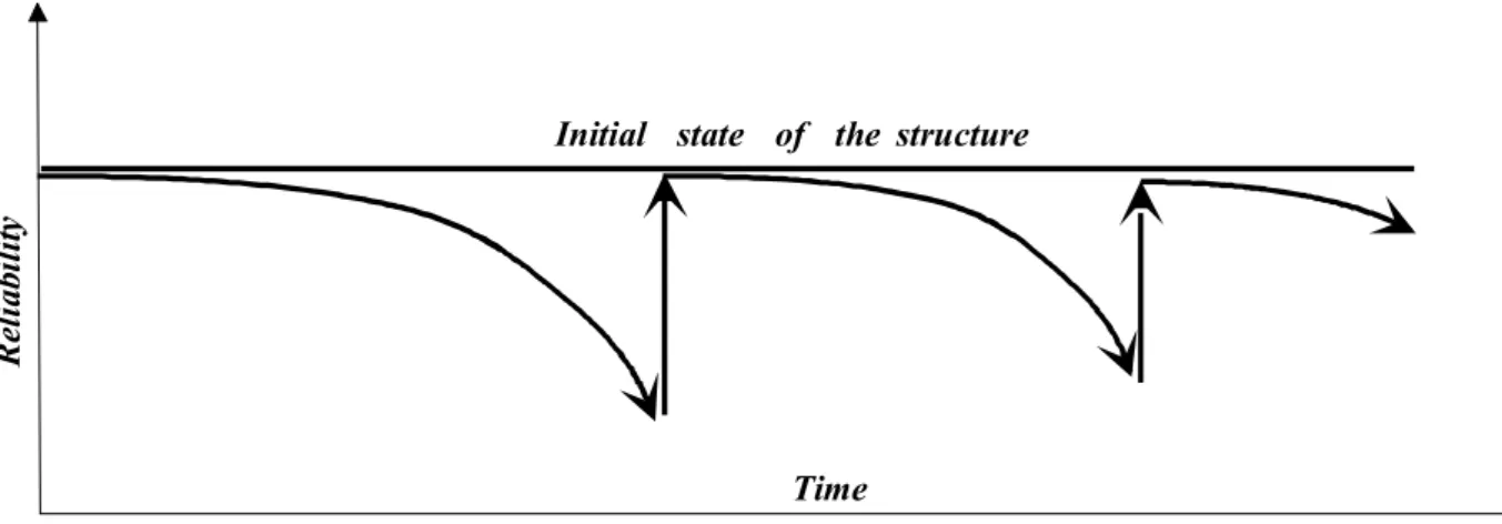
13.3.3. Model of imperfect or bad maintenance: BTO/WTO

In most cases, maintenance operations lead to an improvement of the state of the system, without making it new; we say that the system is “better than old” (BTO). Among the possible reasons for this situation, we can mention imperfections in repair methods, defects induced by the operation itself, the effect of human factors, the impact of the procedures on the rest of the system (e.g. assembly, disassembly), etc. In some cases, maintenance can be bad when the induced errors and defects are significant, if the maintenance staff is not qualified or has insufficient experience, or the working conditions are difficult or inappropriate; in such cases we say that the maintenance is “worse than old” (WTO). Another reason for BTO/WTO maintenance is the application of a “minimal repair time” policy instead of a “minimal repair” policy, in order to increase system availability. Several models have been developed to describe this type of maintenance.

13.3.3.1. Arithmetic Reduction of Age (ARA) model

The Arithmetic Reduction of Age (ARA) model consists of a reduction of the structural age with an amount proportional to the operation time elapsed since the last maintenance action [DOY 04]. In other words, each maintenance operation allows us to reduce the damage developed since the previous maintenance. The age reduction can be obtained by the expression:

(

t Ht

)

h t

(

tι

)

for 0 1 and ti 1 t ti

where

γ

is the efficiency parameter. In this case, the failure rate contains jumps at each maintenance operation. The special cases of minimal or perfect repairs are obtained when the efficiency parameter is equal to 0 or 1, respectively.

13.3.3.2. Non Homogeneous Gamma Process (NHGP)

The effect of imperfect or inefficient maintenance can be considered by assuming that the system is subject to jumps, also called “shocks”, which happen according to a Non Homogeneous Poisson Process (NHPP) of intensity _ρ

( )

t . The failure takes place, not at all the jumps, but only at the k-th jump. For k > 1, the component is in a better state after maintenance and, consequently, the process describes the case of imperfect maintenance. However, for k < 1, the state of the component is degraded after each maintenance operation (i.e. in the case of WTO maintenance). The random variable “numbers of jumps”:

_³

( )

− = i i t t i t dt N 1 ρ is independent and identically distributed according to Gamma law with identical scale and shape parameters, equal to k. The failure rate is given by:

( )

(

(

)

)

(

)

(

)

( )

(

)

(

)

(

_{( )}

(

)

)

1 1 1 1 1 1 1 k i i t i k i i t exp E N t ,t ( t ) E N t ,t k t H for t t exp E N t ,z ( z ) E N t ,z dz k ρ Γ λ ρ Γ − − − − ∞ _{− −} − ª º − ¬ ¼ ª º ¬ ¼ = > ª º − ¬ ¼ ª º ¬ ¼

³

[13.6] with

[

₍

₎

]

_³

_{( )}

− = − t t i i dz z t t N E 1 ,

1 ρ the expectation of the number of jumps between the

last failure and the time t. The process indicated above is called a Non Homogeneous Gamma Process (NHGP). For k = 1, this process is reduced to a Non Homogeneous Poisson Process (NHPP), corresponding to minimal repair; when

( )

t ₌c

ρ , the process becomes a renewal process with times between failures distributed according to Gamma distribution, with scale parameter c and shape parameter k.

13.3.3.3. Lawless-Thiagarajah model

An interesting form of the failure rate which allows the inclusion of time dependence and the effect of observed failures can be written as:

( )

_¸¸ ¹ · ¨ ¨ © § =

¦

= n i i i t g t H t 1 ) ( exp _θ λ [13.7]

where _θi are the model parameters and g_i(t)are functions depending on the time and on the history of the process Ht. Particular forms of this equation can be written:

–

λ

( )

t

H

_t

=

exp

(

α

+

β

t

+

γ

u

(

t

)

)

with

−

∞

<

α

,

β

,

γ

<

∞

–

_λ

( )

_{t H =}

_γ

_tβ−1

( )

_u(_t) δ−1 _with

_γ

_>0,

_β

₊

_δ

_>0

t

–

_λ

( )

t

H

_t

₌

_δ

exp

(

_θ

₊

_β

t

)

[ ]

u

(

t

)

δ−1

with

₋

_∞

_<

_θ

,

_β

_<

_∞

,

_δ

_>

0

where u(t) is a time function. The two last forms of the failure rate are, respectively, associated with renewals of the Weibull and Weibull log-linear models.

13.3.3.4. Arithmetic Reduction of Intensity (ARI) model

Another way to take into account the beneficial effect of maintenance consists of reducing the failure rate, either by a constant quantity, or proportional to the failure rate before maintenance. The intensity reduction can be obtained by:

(

) (

)

0

i i

i _t i _t

t H t H with

λ + + =δ λ − − δ > [13.8]

The parameter

δ

indicates the maintenance efficiency, while

_δ

_<1 corresponds to imperfect maintenance,

_δ

_>1 indicates worse than old maintenance, and

_δ

₌1 corresponds to minimal repair. At the ith failure, the failure rate is written as:

( )

t H_t =δi ρ

( )

t with ti <t ≤ti+1

λ [13.9]

where _{ρ is the failure intensity before the first failure.}

( )

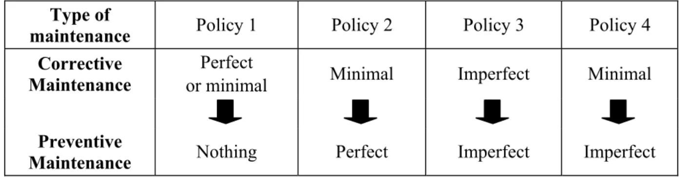
_t

13.3.4. Complex maintenance policy

A complex maintenance policy is made up of a combination of elementary maintenance actions, in order to minimize the cost or to increase availability. Various maintenance policies can be introduced, as summarized in Figure 13.10. 13.3.4.1. Sequence of perfect and minimal repairs, without preventive maintenance

Consider the following case: a structure is repaired when failure occurs, without preventive actions. The system is assumed to be subject to two types of failure: catastrophic with probability p and minor with probability 1-p. The latter is corrected with minimal repair. A Non-homogeneous Poisson Process (NHPP) starts at each perfect repair. The distribution of times between successive perfect repairs is

given as:

( )

[

]

p p t F t

F ₌1₋ 1_{− 1}( ) and the corresponding failure rate is: _λp

( )

t ₌ p_λ1(t).

The intensity is given by:

( )

t

H

_t

=

h

(

t

−

t

i−1

)

with

t

i−1

<

t

≤

t

i

λ

[13.10]

This quantity is numerically equal to the failure rate of the first failure, with age given as t ₋t_i−1.

13.3.4.2. Minimal repairs with perfect preventive maintenance

In this scheme, preventive maintenance renews the state of a structure. In each time interval, a minimal repair is performed when failure occurs. In other words, at each maintenance cycle, a piecewise Non-Homogeneous Poisson Process (NHPP) can be defined. The variations of operating and environmental conditions between different cycles can be considered by introducing a covariance between the cycles:

( )

_¸¸

¹

·

¨¨

©

§

=

¦

j j i j j i

t

h

t

c

t

h

_{, 0}

(

)

exp

_, [13.11]

where h_{i ,j}

( )

t is the failure rate of the “time at the jth failure” during the “ith cycle of maintenance”, t_i,j are the corresponding times and c are regression coefficients. _j

13.3.4.3. Imperfect repairs with perfect preventive maintenance

This scheme consists of performing repairs of type BTO when failure occurs, combined with component renewal during preventive maintenance of type AGAN. This policy represents the case of repairs in difficult conditions, the case of incident events, and complete replacement at planned times as part of preventive maintenance.

Type of

maintenance Policy 1 Policy 2 Policy 3 Policy 4 Corrective

Maintenance

Perfect

or minimal Minimal Imperfect Minimal

Preventive

Maintenance Nothing Perfect Imperfect Imperfect

13.3.4.4. Minimal repair with imperfect preventive maintenance

This policy is probably the closest one to real structures. A minimal repair can always be expected in case of failure, while preventive maintenance cannot often be perfect. This policy aims at minimizing the down time due to failures and consequently maximizing system availability.

13.4. Conclusion

This chapter has introduced the vocabulary related to maintenance of structural components and infrastructures. Corrective or preventive maintenance can be divided into many types of actions, to be selected in an optimal way. The rich literature available should be consulted to provide simple analytical models. These models should be completed to include degradation mechanisms which are defined by complex phenomena with large uncertainties. A solution can therefore be obtained by applying numerical methods and optimization algorithms. The probabilistic approach allows us to take account of uncertainties related to degradation processes and to inspection and maintenance operations.

A probabilistic model of failures and degradations can be a decision-making tool for engineers and decision-makers, allowing the selection of an appropriate maintenance strategy. This choice can be a delicate one, for example, choice between valid techniques for which there is field experience and new techniques for which other advantages are interesting (in terms of performance, economy, etc.).

Finally, throughout the optimization process, we have to be aware of the comparison between the efficiency of various maintenance operations, and the consequences of heavy and delayed investments.

13.5. Bibliography

[CEN 01] CEN, EN 13306, Maintenance Terminology, 2001.

[DOY 04] DOYEN L.,GAUDOIN O.,“Classes of imperfect repair models based on reduction of

failure intensity or virtual age”, Reliability Engineering & System Safety, vol. 84(1), p. 45-56, 2004.

[ELL 97] ELLINGWOOD B.R.,MORI Y., “Reliability-based service life assessment of concrete

structures in nuclear power plants: optimum inspection and repair”, Nucl. Eng. Des., vol. 175, no. 3. p. 247-258, 1997.

[FAB 02a] FABER M.H. “RBI: An Introduction”, Structural Engineering International,

[LAN 05] LANNOY A., PROCACCIA H., Evaluation et maîtrise du vieillissement industriel,

TEC & DOC, Lavoisier, Paris, France, 2005.

[MOR 01] MORI Y.,NONAKA M., “LRFD for assessment of deteriorating existing structures”,

Structural Safety, 23, p. 297-313, 2001.

[NAK 02] NAKANISHI S., NAKAVASU H., “Reliability design of structural system with cost

effectiveness during life cycle”, Comp. and Industrial Engrg, 42, p. 447-456, 2002.

[ZWI 96] ZWINGELSTEIN G., La maintenance basée sur la fiabilité, Hermès Science, Paris,