Formalizing land rights can reduce forest loss:
Experimental evidence from Benin
Liam Wren-Lewis1,2*, Luis Becerra-Valbuena1, Kenneth Houngbedji3
Many countries are formalizing customary land rights systems with the aim of improving agricultural productivity and facilitating community forest management. This paper evaluates the impact on tree cover loss of the first randomized control trial of such a program. Around 70,000 landholdings were demarcated and registered in ran-domly chosen villages in Benin, a country with a high rate of deforestation driven by demand for agricultural land. We estimate that the program reduced the area of forest loss in treated villages, with no evidence of anticipatory deforestation or negative spillovers to other areas. Surveys indicate that possible mechanisms include an increase in tenure security and an improvement in the effectiveness of community forest management. Overall, our results suggest that formalizing customary land rights in rural areas can be an effective way to reduce forest loss while improving agricultural investments.
INTRODUCTION
Rising demand for agricultural land is a major driver of deforesta-tion, contributing to biodiversity loss and climate change (1, 2). A range of actors have long argued that securing the property rights of local populations and improving commons management may help protect forests (3, 4). A recent “Global Call to Action” backed by more than 300 organizations argued that “insecure land rights are a global crisis…undermining our ability to confront climate change” (5). Conservationists have typically concentrated on tenure inter-ventions focused on forests, such as the creation of protected areas. However, the ability of protected areas to preserve forests is limited (6, 7), and there can be important trade-offs between conserving eco-systems in this way and increasing economic activity (8). While many low-income countries have undertaken programs to improve rural land governance, they have often focused on improving the security of agricultural land (9). The impact on forests of such an approach is, however, uncertain (10, 11).
This paper evaluates the impact on forest cover of a large-scale randomized control trial of a rural land rights program undertaken in Benin. The country has one of the highest deforestation rates in the world, having lost approximately a quarter of its forested area between 1990 and 2015 (12). The main cause of this deforestation is expanding agriculture (1, 13). In 2009, the government of Benin rolled out an experimental scale-up of the Plans Fonciers Ruraux (PFR) program with the objective of both increasing agricultural pro-duction and protecting natural resources. The program is a bundle of several interventions broadly serving to formalize and support tra-ditional local land governance systems, lying at the frontier of new land policies being developed in Africa (14).
The random assignment of treated villages in this context pro-vides us with a unique opportunity to identify the causal impact of a land formalization program on forest loss. Previous studies of the impact of land rights on forest loss have generally analyzed reforms that created protected areas or demarcated large areas of forest for community management (15–20). A relatively small number of studies
have looked at the impact of agricultural land rights security on de-forestation, but a recent meta-analysis found that these typically did not construct credible counterfactuals (21).
RESULTS
Land registration program in Benin
The land registration program in Benin, known as the PFR program, demarcated landholdings within villages, documented usage rights, and created institutions to facilitate conflict resolution (see fig. S1 and “Background” section in the Supplementary Materials). The theory behind the intervention was that it would both increase agricultural productivity and improve natural resource management. On the one hand, demarcation and certification would improve farmers’ tenure security on agricultural plots, leading to intensification and a reduc-tion in the need to clear new land. On the other hand, resolving con-flicts, clarifying boundaries, and documenting usage rights would re-duce the transaction costs involved in cooperation. This enhanced cooperation could then facilitate the effective self-governance of common-pool resources including forests (3).
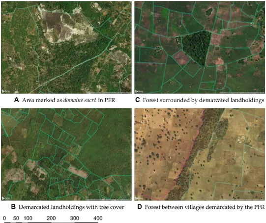
Most of the landholdings demarcated by the PFR program con-tained agricultural plots, but forested areas were also demarcated in several ways. At times, areas of communally managed forest are documented explicitly in the PFR—as an example, Fig. 1A shows a demarcated area with some tree cover labeled explicitly as a domaine sacré (sacred ground) within the PFR. In a similar vein, we also find de-marcated areas within the PFRs labeled as domaine du village (village land) or réserve villageoise (village reserve). Areas of forest also frequently occur on areas registered in an individual’s name, such as those in Fig. 1B, although even here, typically, the individual is described as a representative of a lineage or collectivité. This means that there is a substantial amount of tree cover within the demarcated areas— according to our highest resolution measure of tree cover (from RapidEye), 12% of pixels within the demarcated areas are classified as trees in the baseline year, which is very similar to the tree cover in the 5-km buffers that we use in our main analysis. Even when for-ested areas are not included within the PFR, they may be effectively demarcated by the program. For instance, Fig. 1C shows a small forest that is encircled by demarcated landholdings, while Fig. 1D displays an area of forest that lies between two demarcated villages. 1Paris School of Economics, 48 Boulevard Jourdan, Paris 75014, France. 2INRAE, 147
rue de l'Université, Paris 75007, France. 3DIAL, LEDa, Université Paris-Dauphine, IRD, Université PSL, 4 Rue d’Enghien, Paris 75010, France.
*Corresponding author. Email: [email protected]
The Authors, some rights reserved; exclusive licensee American Association for the Advancement of Science. No claim to original U.S. Government Works. Distributed under a Creative Commons Attribution NonCommercial License 4.0 (CC BY-NC). on June 28, 2020 http://advances.sciencemag.org/ Downloaded from
Overall, therefore, the PFR program effectively demarcated many forested areas in addition to agricultural plots.
Impact of the PFR program on tree cover loss
Our evaluation exploits the randomized rollout of the PFR program across the country. The program selected 575 eligible villages across the country and then organized 80 lotteries to randomly pick 300 vil-lages for treatment (fig. S2). Activities began in treatment vilvil-lages in 2009, and to this date, the program has not been expanded to the con-trol villages (fig. S3 provides a timeline).
We measure the impact on forest loss using three different sources (see “Data” section for more details—summary statistics are given in table S1). Our primary measure is from a publicly available data-set of global annual forest loss between 2000 and 2017 constructed by Hansen et al. (22) from Landsat satellites. We also construct our own measure of forest loss from 2010 using higher-resolution data from RapidEye satellites (23). Last, we analyze the impact on fires measured by MODIS (Moderate Resolution Imaging Spectroradiometer) satellites (24) because fires are commonly used to clear land in Benin.
We construct an annual village-level panel by aggregating forest loss and fires within nonoverlapping 5-km buffers centered on the villages (fig. S4). Because the area of forest loss and number of fires are highly skewed (fig. S5), we use the inverse hyperbolic sine (IHS) of each variable. We estimate the impact of the PFR with the follow-ing ordinary least squares regression
¯
Y v,post = l Treat v + ¯ Y v,pre + X v + l + ϵ v (1)
where ¯ Y v,post is the average of the outcome variable over the
post-treatment years (2009 to 2017), l is the treatment effect on villages in
lottery l, ¯ Y v,pre is the average of the outcome variable over the
pre-treatment years (2001 to 2008), and Xv is a set of village-level controls
including those variables found to be unbalanced across treatment and control groups. Note that we cannot control for the pretreatment average when we use the RapidEye measure of forest loss as we have no data from before 2010, so instead, we control for pretreatment forest loss as measured by Landsat. In regressions using forest loss, we additionally control for forest cover at baseline. Because the treat-ment probability varies across lotteries, we estimate separate treattreat-ment effects l for each lottery l and then present the average treatment
effect weighting l by the share of villages in lottery l (25).
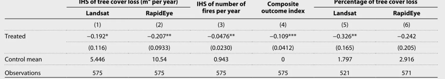
The main findings of our work are presented in Table 1. The table shows that the PFR treatment reduced forest loss and fires in the areas containing treated villages. More precisely, the point estimates in columns 1 to 3 suggest a reduction in tree cover loss of around 20% and a reduction in fires of 5% (26). Using the Landsat measure, we estimate that 2700 ha of tree cover was lost in the treated villages between 2009 and 2017, and hence, the point estimate suggests that the program led to 600 ha of extra tree cover by the end of 2017. When we construct a composite index using information from all three of these variables in column 4, we estimate a reduction in the
A C
B D
m
Fig. 1. Examples of forested areas demarcated by PFRs. This figure gives examples of areas containing tree cover that have been effectively demarcated by PFRs.
Hatched areas correspond to demarcated landholdings with entries labeled within the village PFR and solid lines display the recorded borders of these landhold-ings. Panel (A) shows a demarcated sacred ground. Panel (B) shows demarcated private landholdings with tree cover. In (C) we see a communal forest surrounded by demarcated landholdings. Panel (D) shows a forest spreading between villages demarcated by the PFR; the two colors represent two adjacent treated villages. Photo credit: Microsoft Bing Maps Aerial.
on June 28, 2020
http://advances.sciencemag.org/
treatment group of around 11% of an SD. In columns 5 and 6, we take the annual percentage of tree cover loss as our outcome variable and find a reduction of 0.1 to 0.3 percentage points. For the Landsat measure, the coefficient implies that the percentage of tree cover lost is 18% lower than in control villages.
We conducted several further analyses to assess the robustness of the results (see “Robustness checks” section for more details). The robustness checks included using buffers of 3 or 10 km rather than 5 km (table S2a), making the dependent variable the villages’ rank within the sample instead of the IHS (table S2b), using alternative sets of control variables (table S3a) and calculating P values using randomization inference (table S3b). In all these cases, the magnitude and significance of the coefficients of interest remain largely unchanged. We also interact the treatment dummy with predetermined observable vari-ables and find no clear pattern of treatment effect heterogeneity (table S4).
Are there negative spillover effects?
Might the reduction in tree cover loss be the result of a displace-ment rather than a net reduction in tree cover loss? This could occur in two ways. First, tree cover loss may be displaced over time if villagers anticipate the formalization and clear land beforehand. Second, tree cover loss may be displaced geographically if the program makes it relatively harder to clear trees in the treated village.
To investigate the possibility of temporal displacement, we first undertake our analysis at the monthly level using data on the number of fires (see “Displacement and spillovers” section in the Supplemen-tary Materials and Methods for more details). We find no significant impact of treatment on fires in the months in between the informa-tion campaign and formalizainforma-tion (table S5a). We also see no evidence of anticipatory deforestation when we plot annual regression coeffi-cients (fig. S7). Last, we find no evidence of greater tree cover loss or fires during the period of the information campaign in those areas where it took place (table S5b).
To test for spatial displacement, we first consider spillovers to nearby villages by estimating the impact of villages within 5 km having been treated (table S6). We find no evidence of negative spillovers in either treatment or control villages. We also find no evidence of greater forest loss or fires in areas that are near treated villages but were probably not demarcated (table S7).
What explains the reduction in tree cover loss?
Evidence from the pattern of tree cover loss and survey data suggests three likely mechanisms through which the PFR program reduced
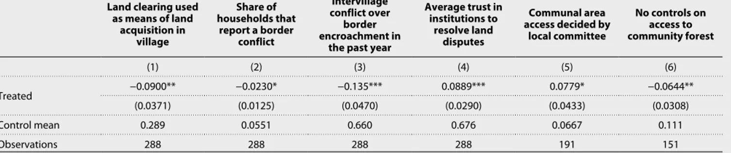
tree cover loss. First, the program may have increased farmers’ in-vestment in existing plots, increasing productivity and, hence, reduc-ing the need to clear further land. This is supported by the results of two other studies that found the program led to increased investment (14, 27). We also find evidence consistent with this in our analysis of community surveys, which are reported in Table 2. The regres-sions in this table use the same estimation technique as outlined in Eq. 1 but are restricted to the smaller set of villages that were sur-veyed in 2011. In column 1 of Table 2, we regress a binary variable that takes a value of 1 if the community leader interviewed reported land clearing as a technique that was used in the village to acquire land. We can see that this is significantly less likely to be the case in treated villages. We also find a significant reduction in tree cover loss directly adjacent to agricultural plots, which is likely to be the area most at risk from the expansion of agriculture (panel b of table S8).
Second, the increase in tenure security may have guaranteed farmers that they had enough land for future production, and hence reduced the incentive to claim land through clearing. In column 2 of Table 2, we note that treated villages are significantly less likely to experience border conflicts, presumably as a result of the demar-cation process. In our qualitative survey, one interviewee responded that “since the project placed markers, everybody knows their parcels and there are no more land problems.” This mechanism may have operated both at an individual level and at the level of the village. In column 3 of Table 2, we note that community leaders are significantly less likely to report that their village has a conflict with a neighbor-ing village over border encroachment in the past year. This fall in intervillage conflict is therefore likely to have reduced the incentive of villagers to clear land on disputed village boundaries to enhance their claims.
Third, the delimitation of landholdings and the creation of local land committees are likely to have reduced the transaction costs of commons management. We see in column 4 of Table 2 that treated villages report a significantly higher level of trust in institutions to resolve land conflicts. Moreover, respondents in treated villages were significantly more likely to say that communal areas were managed by a local committee such as the conseil du village, rather than an individual (column 5 of Table 2). This is consistent with the PFR pro-gram’s stated aim of encouraging participation in land governance (28). We also observe in column 6 of Table 2 that treated villages are significantly more likely to restrict access to communal forests than control villages. The qualitative interviews we undertook in 2017 sug-gest that restrictions on land clearing such as these were effective,
Table 1. Effect of the PFR program on tree cover loss and number of fires. The composite outcome index, in column 4, is formed by taking the average of
the z scores of the dependent variables in columns 1 to 3. SEs are heteroskedasticity robust.
IHS of tree cover loss (m2 per year)
IHS of number of
fires per year outcome indexComposite
Percentage of tree cover loss
Landsat RapidEye Landsat RapidEye
(1) (2) (3) (4) (5) (6)
Treated −0.192* −0.207** −0.0476** −0.109*** −0.326** −0.242
(0.116) (0.0933) (0.0230) (0.0412) (0.165) (0.205)
Control mean 5.446 10.54 0.943 0 1.797 2.916
Observations 575 575 575 575 521 571
Asterisks denote significance: *P < 0.10, **P < 0.05, and ***P < 0.01.
on June 28, 2020
http://advances.sciencemag.org/
with one interviewee telling us that “Today you can’t go clear land like before. If you want more land to cultivate, you can go rent the demarcated plot of another villager.”
DISCUSSION
Curbing deforestation is a major environmental challenge, and ad-dressing it requires assessing the effectiveness of a range of policies and understanding the mechanisms behind their successes or failures. This paper demonstrates that land formalization programs focused on agricultural land can generate an important positive externality in reducing forest loss. We find no evidence that formalization dis-placed deforestation. Instead, the results from qualitative and quan-titative household surveys suggest that land registration activities reduced deforestation in Benin by (i) increasing agricultural pro-ductivity on existing plots, (ii) reducing the need to clear existing forested land to signal and safeguard private land rights, and (iii) im-proving land governance and the action of communal management of forest resources.
While these results are estimated on a selected sample of villages, we find no consistent evidence that the effects vary systematically by village characteristics. We cannot, however, directly infer the ex-tent to which the results are generalizable to other contexts, and more studies are therefore required to identify how deforestation impacts will vary in other countries. Because deforestation trends are driven by several factors and there is likely no silver bullet to address them all, policy makers would be advised to adopt several approaches de-pending on local contexts. In this sense, land formalization may be an important complement to other programs, which have been shown to be effective elsewhere, such as payments for ecosystem services (29). Programs such as these often rely on defining who is responsi-ble for the management of a given forest and therefore implicitly formalize a system of rights. In this context, it is important to have evidence on the direct impact of the formalization process on deforestation.
MATERIALS AND METHODS
Experimental design
The Millenium Challenge Corporation (MCC)–supported PFR program aimed to produce 300 censuses of landholdings and land rights held in
rural villages across 40 communes throughout Benin (communes are subregional units equivalent to districts—there are 77 communes in Benin). Selection into the program was done in three steps. First, all villages in each of the 40 communes received an information campaign. The intention was to inform villages about the program and invite them to apply for a chance to receive 1 of the 300 PFRs. Second, proposals were reviewed against preestablished selection criteria. The following criteria were used: poverty index, potential for commercial activities, regional market integration, local interest in promoting gender equality, infrastruc-ture for economic activities, adherence to the PFR application pro-cedures, incidence of land conflicts, and production of main crops. From this review, a list of eligible villages was produced. Third, each commune organized lotteries to randomly select villages within the eligible pool into the program.
Overall, around 1200 villages applied for the program, out of the 2062 that were informed. Of these 1200 villages, 575 met the eligi-bility criteria. These 575 villages that were part of the lotteries are not representative of all villages in Benin—they are, for instance, more rural, more ethnically diverse, and report a greater number of land conflicts than ineligible villages. This is not a problem for our iden-tification because we only look at differences between eligible villag-es, but it may be a concern for external validity. We therefore pay attention to these variables when we test for heterogeneous treatment effects (see “External validity and heterogeneity” section in the Sup-plementary Materials and Methods for more details). Moreover, we construct a propensity score for each village estimating how likely it would be deemed eligible based on observable characteristics and test for whether the treatment effect is heterogeneous in this variable.
To select treatment and control villages, the implementing agency of the MCC in Benin organized 80 public lotteries, 2 in each commune. Each pair of lotteries was structured to allow for villages sampled in the 2006 national household survey [Enquête modulaire integrée sur les conditions de vie (EMICoV)] to be overrepresented in the program, thus allowing for the EMICoV survey to be used for evaluation purposes. Because the EMICoV survey uses a random sampling strategy at the commune level, this should not affect the validity of our identification. We account for this lottery stratification in our econometric analysis. Figure S2 shows the different steps of the selection process. Land demarcation activities were undertaken in 98% of the treated villages and only in 2 of the 275 control villages. The two control villages that received land de-marcation activities served as replacement villages for two of the
Table 2. Impact on variables in the 2011 community and household surveys. This table considers impacts on various questions asked to community leaders
and surveyed villagers. The samples in columns 1 to 4 include those villages surveyed in 2011. In columns 5 and 6, we restrict the included villages to those that reported having communal areas or community forest, respectively. SEs are heteroskedasticity robust.
Land clearing used as means of land acquisition in village Share of households that report a border conflict Intervillage conflict over border encroachment in
the past year
Average trust in institutions to resolve land disputes Communal area access decided by local committee No controls on access to community forest (1) (2) (3) (4) (5) (6) Treated −0.0900** −0.0230* −0.135*** 0.0889*** 0.0779* −0.0644** (0.0371) (0.0125) (0.0470) (0.0290) (0.0433) (0.0308) Control mean 0.289 0.0551 0.660 0.676 0.0667 0.111 Observations 288 288 288 288 191 151
Asterisks denote significance: *P < 0.10, **P < 0.05, and ***P < 0.01.
on June 28, 2020
http://advances.sciencemag.org/
lotteries.
Goldstein et al. (14) analyze the short-term impact on household agricultural activity. They find an increase in investment on treated parcels, with important heterogeneity across genders. In particular, female-managed landholdings in treated villages are more likely to be left fallow. The surveys used in this analysis did not ask questions about uncultivated plots or deforestation directly, but we use some questions in the survey to document how land registration activities have changed land management practices at the communal levels to produce the results in Table 2.
Data
The first step in constructing our dataset is to locate all the 575 eli-gible villages. For 283 of the villages, we can use the GPS coordinates of cultivated plots, which were surveyed by Goldstein et al. (14), and we take the village centroid to be the center of the surveyed plots. For the remaining villages, we use a combination of sources, because no single source contains the location of all our villages. These sources include data from the Institut National de la Statistique et de l’Analyse Économique (INSAE), the location of infrastructure projects col-lected by EMICoV, and maps from l’Institut Géographique National du Bénin (IGN-Bénin) and INSAE. We estimate the quality of each source on the basis of how close the coordinates are to the centroids calculated in the surveyed villages and locate each village according to the highest-quality source, which gives a position of the village.
We then construct buffers around each village. We do not make use of village maps, because we do not have maps of village bound-aries for the control villages, and, instead, use the same procedure for treatment and control villages. These are circles with a 5-km diameter by default, which we ensure to be nonintersecting by as-signing areas to the closest village when within 5 km of more than one village. These buffers are displayed in fig. S4. The 5-km figure is somewhat arbitrary, and we therefore test for robustness to alternative distances. The buffers generally seem consistent with the surveyed plot data—see the villages in fig. S8, for example—but we do not con-struct buffers based on the surveyed plot data because the surveyed plots are likely to be unrepresentatively close to the village centers.
Our primary measure of forest loss comes from version 1.5 of the Global Forest Change dataset constructed by Hansen et al. (22) us-ing Landsat satellite data. For each 30 m × 30 m pixel globally, they construct a measure of forest cover in 2000 and whether each pixel experienced forest loss between 2000 and 2017. To reduce noise, we only consider grid cells with more than 25% forest cover in 2000, in accordance with previous work using this data (30, 31). To calculate the total forest loss within a village buffer, we weigh pixels by the percentage of forest cover in 2000—deforestation of a pixel that had 80% forest cover therefore counts for double that of a pixel that had 40% forest cover. In this way, we form an estimate of the total area of forest loss within a village buffer for each year between 2001 and 2017.
Our second outcome measure estimates tree cover loss using data from the RapidEye satellites, which have a 5-m pixel resolution. For each village, we compared two images taken between December and February (the driest season) in different years to estimate tree loss between the earliest year possible and 2016. For the northern part of the country, it was possible to use images from 2010, but for the southern part, the earliest usable images were from 2012. The pixels were then classified using supervised classification by maximum likelihood estimation to obtain maps of vegetal cover. Pixels were then
sified as forest in the earlier year to bare soil in the latter year. Our village-level measure is the total area of the pixels classified as suf-fering tree cover loss between the 2 years divided by the number of years between the images.
In addition to measuring forest loss directly, we also use data on fires because burning is a key tool in forest clearance and is generally correlated with deforestation. Data on fires are from the MODIS Collection 6 Active Fire Product (24). This product detects fires in 1-km pixels that are burning at the time of overpass under relatively cloud-free conditions using a contextual algorithm, where thresh-olds are first applied to the observed middle-infrared and thermal infrared brightness temperature, and then false detections are re-jected by examining the brightness temperature relative to neighboring pixels. We sum the number of fires within each buffer for each year between 2002 and 2017, weighting fires by the confidence measure calculated by Giglio et al. (24).
We use all three of these measures in our main analysis because each source has its relative advantages. One potential problem with using direct tree cover loss measures is that they do not distinguish between permanent deforestation and temporary clearances (1). We observe in our tree cover loss data patterns that appear to be the result of managed logging, which we would not anticipate being affected by the PFR program. An advantage of using data on fires is that fires are not used to clear in this way and, hence, are more likely to be correlated with the kind of tree cover loss we are most interested in. A further advantage of using the fire data is that the observation frequency is much higher. Although the Hansen et al. data assign a year to any measured forest loss, in their validation exercise, they find the year only accords with MODIS data 75.2% of the time (22). The main advantage of the RapidEye-based measure is that it has a much higher resolution than the measure derived by Hansen et al. This is particularly helpful when analyzing where tree cover loss occurred near plot boundaries, because the 30-m pixels often span both sides of a demarcated boundary. An additional advantage of these data is that we calibrated the measure using imagery from Benin only, and hence, it may be more sensitive to changes in tree cover than the Hansen et al. measure, which has global cover. When we correlate the relevant variation in the three measures in the posttreatment period, we find the two measures of forest loss have a correlation of 0.33 with each other, and both have a correlation of 0.24 with the measure of fires. This suggests that they bring different information to the analysis. We therefore also construct a composite index containing information from all the available outcome measures—further de-tails can be found below in the “Econometric specification” section. In table S1, we present summary statistics of various variables for the period 2001 to 2008 across treatment and control villages. Note that, according to our tree cover measure constructed using the Global Forest Change data, the average village had around 80 ha of tree cover in 2000 but had lost roughly 1 ha each year before 2009. This annual rate of forest loss of around 1.25% is slightly higher than the national rate according to the Hansen et al. data, which is 0.8%. Both are comparable to the 1% national rate estimated by the Food and Agriculture Organization of the United Nations over a similar period (12).
Econometric specification
The random assignment of the program at the village level establishes our identification, and we exploit within-lottery variation to estimate the average treatment effect of being selected for the PFR program.
on June 28, 2020
http://advances.sciencemag.org/
As displayed in Eq. 1, we estimate a vector of treatment effects, one for each lottery, and then take the weighted average of these, which produces an unbiased and consistent estimate of the average treat-ment effect (25).
We test for balance across treatment and control groups in column 5 of table S1 by undertaking the regression detailed in Eq. 1 with various predetermined variables as the outcome variable. In this case, the set of control variables Xv includes only lottery dummies and an
indicator of whether the village was surveyed or not. We control for lottery fixed effects because the probability of treatment varies across lottery. The source used to determine the village’s location is also cor-related with a village’s treatment status, because treated villages are more likely to be surveyed, and where possible, we use the surveys to locate the villages.
In general, we can see that most variables are balanced across the two samples—of the 40 variables we include, we find significant dif-ferences at the 10% level for only 4 of them and at the 5% level for only 1. This is consistent with the balance found across previously surveyed villages by Goldstein et al. (14). We include the four un-balanced variables—namely, total tree cover in the village buffer, the distance to the nearest protected area, the share of houses with met-al roofs, and whether the village is classified as urban—in the vector of control variables Xv in all the following regressions unless
other-wise stated.
Independently of the satellites used, our main variables of inter-ests show that the distributions of area deforested and the number of fires per buffer are highly skewed. For instance, 95% of our obser-vations have an area of tree loss of less than 5 ha, but our maximum value is more than 100 ha. Similarly, while the median observation has less than one fire (adjusted for confidence), the top 1% of our observations have more than 15 fires. If we regress these variables linearly on treatment status, results are likely to be driven by these outliers. This is concerning to us because we believe these outliers may well be the result of measurement error and will therefore sim-ply add noise—a large amount of forest loss, for instance, may be the result of the cutting of a plantation, while a large number of observed fires may represent repeated observations of the same out of control wildfire rather than repeated land clearances.
In our main analysis, we therefore use the IHS of each of these variables. Transforming skewed data to reduce the influence of ex-treme values and comply with the normality assumptions of linear regression models is good practice (32–35), and the IHS is widely used because it approximates the natural logarithm while allowing the retention of zero-valued observations (26, 36).
To accommodate other possible transformations, our baseline specification includes three more outcome variables in addition to the IHS of the measures described above. First, we construct a com-posite outcome index, which combines the information in the first three outcome variables. In particular, we convert the three initial outcome measures into z scores by subtracting the mean and divid-ing by the SD, and then we take the average of the available scores to produce a combined index. We then demean and divide this index by the SD to ease interpretation. Second, for our measures of tree cover loss, we divide by baseline tree cover instead of taking the IHS. This creates two measures of the percentage of tree cover loss, re-ducing skewness caused by large variations in baseline tree cover. Note, however, that this can lead to extreme values when villages have a small amount of tree cover. For instance, there is one village in the treatment group that lost 45% of its tree cover according to
Rapid-Eye (no other village lost more than 20%)—the village in question only has 475 m2 of tree cover, the sixth lowest in our sample. Note
also that the percentage of tree cover lost is undefined for areas that had no tree cover at baseline, and therefore, the number of observa-tions is typically smaller in regressions with this outcome measure. For both measures of tree cover, we do not find any significant dif-ference in the number of villages with no cover when we check for balance in the same way as we do for other variables in table S1.
Robustness checks
Table S2b considers how sensitive our results are to our choice of dependent variable. An alternative methodology to reduce the in-fluence of outliers is to rank villages each year according to the out-come measure, normalize the rank around zero, and then take this as the dependent variable. The results of this process are reported in columns 1 to 3, and we note that there is still a statistically signifi-cant impact of treatment for two of the three measures. The coefficient using the RapidEye measure of tree loss is insignificant, but it is not significantly different from either of the coefficients in columns 1 and 3—in all three cases, it appears that treatment reduces the rank-ing of treated villages by around 10 places. One way of interpretrank-ing these coefficients is to ask what percentage decrease in the base out-come variable in the control group would have led to a coefficient of zero in these regressions. For the case of tree cover loss measured by Landsat, for instance, we find this to be a 20.3% reduction in tree cover loss, which is very similar to the magnitude we estimated in the base-line specification. In columns 4 to 6, we consider an extreme trans-formation whereby we simply record whether any forest loss—or any fires—are recorded in the village buffer each year. In this case, we find small insignificant coefficients, which suggests that the vari-ation driving our result is on the intensive margin. This is perhaps not unexpected given that, on average, villages experience tree cov-er loss/fires in most years. In columns 7 to 10, we use the raw out-come measures, which we know to be highly skewed. When we use an ordinary least square (OLS) regression in columns 7 to 9, the coefficients are insignificant, consistent with this specification being vulnerable to extreme values unrelated to the PFR program. We see that there is one village in the treatment group, Ologo, that experi-enced more than a hundred times the median amount of deforesta-tion between 2009 and 2017. Looking at the satellite data, we can see that this cannot be a result of the treatment—instead, it is driven by the cutting of a large-scale industrial plantation that was near the vil-lage but not part of the PFR program. For the number of fires, as well as using the OLS, we can also undertake a Poisson regression, be-cause the raw fire measure is at its base a count variable. We do this in column 10, and here, the coefficient is statistically significant at the 10% level and corresponds to an incidence rate ratio of 0.93, mean-ing that treatment led to a 7% reduction in the number of fires. This estimate is very close to that of the baseline specification in Table 1.
We may also wonder how robust our measure is to using alter-native sources of forest cover data. We therefore construct a measure of forest cover loss using the MODIS Vegetation Continuous Fields product (37). This product estimates forest cover continuously each year within 250-m pixels. Because the resolution is much lower than Landsat or RapidEye, we do not measure tree loss as going to 0% tree cover but instead measure the number of pixels in which there was a significant reduction in forest cover, calculated using the pixel- level SDs that the product supplies. Column 11 of table S2b then reports the results when we take the IHS of the area, which observed
on June 28, 2020
http://advances.sciencemag.org/
simply measure whether any pixels experienced significant tree loss. In both cases, we obtain coefficients very similar to those estimated when using the Global Forest Change product produced by Hansen
et al. (22).
Table S3a considers how robust our results are to using alterna-tive sets of control variables. In panel 1, we include only the pretreat-ment average outcome as a control variable, removing the other variables that are included in the baseline specification (i.e., those variables that are unbalanced at baseline). In panel 2, we replace the control variables that were previously in Xv with the full set of
30 predetermined variables, which are listed in table S1. In panel 3, we then use the “post–double selection” lasso technique to select the most relevant control variables from among this set of 30 and their interactions (38, 39). In all three cases, we can see that our results generally do not change substantially and remain significant.
Another concern is that our SEs may be inappropriate given spatial correlation in both the treatment and the outcome variables. In panel 3 of table S3b, we therefore present SEs calculated in two alternative ways. In parentheses below, the coefficients are SEs, which allow for spatial correlation over 10 km using the Stata routine reg2hdfespa-tial developed by Thiemo Fetzer, based on the method developed by Hsiang et al. (40) and Conley (41). Below this, we then give the P values using randomization inference. These are calculated by per-muting the assigned treatment status across villages 1000 times using the Stata command ritest and then calculating the regression coeffi-cient in each case (42). We can note that P values remain very close to those in the baseline specification.
In panel 4 of table S3b, we estimate the average treatment effect using inverse probability weighting (IPW) instead of estimating lottery-specific treatment effects. We do not include lottery-fixed effects but instead weigh each observation as follows. Each treated observation is weighted by the inverse of the proportion of villages in the lottery who were assigned to the treatment condition, and each control village is weighted by the inverse of the proportion of villages in the lottery who were assigned to the control condition. Note that eight villages are assigned zero weight and are therefore dropped from the regression, because they are in lotteries where all villages were treated. This occurred because of quotas on the required num-ber of villages to be treated within each lottery. These villages do not contribute directly to the estimated treatment effect in our main spec-ification but remain in the regression because they influence the esti-mated coefficients on the control variables. We can see from the table that coefficients estimated using IPW are very similar to those esti-mated using our main technique. The SEs given by IPW are typically slightly larger than those in Table 1, but the P values given through randomization inference are very similar.
Figure S6 displays dot plots of the first four outcome variables. These are constructed according to the technique outlined in Gerber and Green (43), whereby we first regress both the outcome variable and the treatment status on the set of controls in separate regressions. We then plot the average of the residuals within each group (treatment and control within each lottery) against the average of the residual of the treatment status within this group. The size of the circle plotted corresponds to the sum of the normalized inverse probability weights within each group—this is equal to the num-ber of villages in the corresponding lottery. Plotting the variables in this way gives us a sense of what the treatment effect looks like. We can first note that the treatment effect is small relative to the
varia-in column 4 of Table 1, for varia-instance, we estimate the treatment effect on the composite outcome index to be 10% of the SD across villages. A second point we can note from this figure is that the re-sults do not appear to be driven by outliers. While there are groups with large residual values both above and below the mean, these do not appear to be consistently driving the difference between the treatment and control groups.
SUPPLEMENTARY MATERIALS
Supplementary material for this article is available at http://advances.sciencemag.org/cgi/ content/full/6/26/eabb6914/DC1
View/request a protocol for this paper from Bio-protocol.
REFERENCES AND NOTES
1. P. G. Curtis, C. M. Slay, N. L. Harris, A. Tyukavina, M. C. Hansen, Classifying drivers of global forest loss. Science 361, 1108–1111 (2018).
2. J. Barlow, F. França, T. A. Gardner, C. C. Hicks, G. D. Lennox, E. Berenguer, L. Castello, E. P. Economo, J. Ferreira, B. Guénard, C. G. Leal, V. Isaac, A. C. Lees, C. L. Parr, S. K. Wilson, P. J. Young, N. A. J. Graham, The future of hyperdiverse tropical ecosystems. Nature 559, 517–526 (2018).
3. E. Ostrom, Self-governance and forest resources. CIFOR Occ. Paper 20 (1999). 4. Ö. Bodin, Collaborative environmental governance: achieving collective action
in social-ecological systems. Science 357, eaan1114 (2017).
5. F. Pearce, Common Ground: Securing Land Rights and Safeguarding the Earth (Oxfam International, Oxford, 2016).
6. F. M. Pouzols, T. Toivonen, E. Di Minin, A. S. Kukkala, P. Kullberg, J. Kuusterä, J. Lehtomäki, H. Tenkanen, P. H. Verburg, A. Moilanen, Global protected area expansion is
compromised by projected land-use and parochialism. Nature 516, 383–386 (2014). 7. J. E. Watson, N. Dudley, D. B. Segan, M. Hockings, The performance and potential
of protected areas. Nature 515, 67–73 (2014).
8. E. G. Frank, W. Schlenker, Balancing economic and ecological goals. Science 353, 651–652 (2016).
9. F.F.K Byamugisha, Securing Africa’s Land for Shared Prosperity (World Bank, Washington DC, 2013).
10. J. M. Baland, J. P. Platteau, Halting Degradation of Natural Resources: Is There a Role for Rural Communities? (Oxford Univ. Press, 2000).
11. B. E. Robinson, Y. J. Masuda, A. Kelly, M. B. Holland, C. Bedford, M. Childress, D. Fletschner, E. T. Game, C. Ginsburg, T. Hilhorst, S. Lawry, D. A. Miteva, J. Musengezi, L. Naughton-Treves, C. Nolte, W. D. Sunderlin, P. Veit, Incorporating land tenure security into conservation. Conserv. Lett. 11, 12383 (2018).
12. Food and Agriculture Organization, Global Forest Resources Assessment 2015: How Are The World’s Forests Changing? (Food and Agriculture Organizations, Rome, 2015).
13. J. E. Bidou, I. Droy, R. Houesse, C. Mering, Dynamiques démographiques, vulnérabilité et évolution du couvert végétal au nord Bénin: Des interactions complexes. Espace. Popul. Soc. 10.4000/eps.8083 , (2019).
14. M. Goldstein, K. Houngbedji, F. Kondylis, M. O’Sullivan, H. Selod, Formalization without certification? Experimental evidence on property rights and investment. J. Dev. Econ. 132, 57–74 (2018).
15. J. Alix-Garcia, L. L. Rausch, J. L’Roe, H. K. Gibbs, J. Munger, Avoided deforestation linked to environmental registration of properties in the Brazilian Amazon. Conserv. Lett. 11, e12414 (2018).
16. A. Blackman, L. Corral, E. S. Lima, G. P. Asner, Titling indigenous communities protects forests in the Peruvian Amazon. Proc. Natl. Acad. Sci. U.S.A. 114, 4123–4128 (2017). 17. M. T. Buntaine, S. E. Hamilton, M. Millones, Titling community land to prevent
deforestation: An evaluation of a best-case program in Morona-Santiago, Ecuador. Glob. Environ. Chang. 33, 32–43 (2015).
18. T. Fetzer, S. Marden, Take what you can: Property rights, contestability and conflict. Econ. J 127, 757–783 (2017).
19. G. Vergara-Asenjo, C. Potvin, Forest protection and tenure status: The key role of indigenous peoples and protected areas in Panama. Glob. Environ. Chang. 28, 205–215 (2014).
20. B. Nolte, B. Gobbi, Y. L. Polain, de Waroux, M. Piquer-Rodríguez, V. Butsic, E. F. Lambin, Decentralized land use zoning reduces large-scale deforestation in a major agricultural frontier. Ecol. Econ. 136, 30–40 (2017).
21. B. E. Robinson, M. B. Holland, L. Naughton-Treves, Does secure land tenure save forests? A meta-analysis of the relationship between land tenure and tropical deforestation. Glob. Environ. Chang. 29, 281–293 (2014).
on June 28, 2020
http://advances.sciencemag.org/
22. M. C. Hansen, P. V. Potapov, R. Moore, M. Hancher, S. A. Turubanova, A. Tyukavina, D. Thau, S. V. Stehman, S. J. Goetz, T. R. Loveland, A. Kommareddy, A. Egorov, L. Chini, C. O. Justice, J. R. G. Townshend, High-resolution global maps of 21st-century forest cover change. Science 342, 850–853 (2013).
23. Planet Team, Planet Application Program Interface: In Space for Life on Earth (Planet Team, San Francisco, CA, 2017).
24. L. Giglio, W. Schroeder, C. O. Justice, The collection 6 MODIS active fire detection algorithm and fire products. Remote Sens. Environ. 178, 31–41 (2016).
25. C. E. Gibbons, J. C. S. Serrato, M. B. Urbancic, Broken or fixed effects? J. Econometric Meth.
8, 1–12 (2018).
26. M. F. Bellemare, C. J. Wichman, Elasticities and the inverse hyperbolic sine transformation. Oxf. Bull. Econ. Stat. 82, 50–61 (2019).
27. R. H. Yemadje, T. A. Crane, R. L. Mongbo, A. Saïdou, H. A. Azontonde, D. K. Kossou, T. W. Kuyper, Revisiting land reform: Land rights, access, and soil fertility management on the Adja Plateau in Benin. Int. J. Agr. Sustain 12, 355–369 (2014).
28. P. Lavigne-Delville, La réforme foncière rurale au Benin. Émergence et mise en question d’une politique instituante dans un pays sous régime d’aide. Revue Française De Science Politique 60, 467–491 (2010).
29. S. Jayachandran, J. de Laat, E. F. Lambin, C. Y. Stanton, R. Audy, N. E. Thomas, Cash for carbon: A randomized trial of payments for ecosystem services to reduce deforestation. Science 357, 267–273 (2017).
30. M. C. Hansen, S. V. Stehman, P. V. Potapov, Quantification of global gross forest cover loss. Proc. Natl. Acad. Sci. U.S.A. 107, 8650–8655 (2010).
31. A. Leblois, O. Damette, J. Wolfersberger, What has driven deforestation in developing countries since the 2000s? Evidence from new remote-sensing data. World Develop. 92, 82–102 (2017).
32. J. M. Wooldridge, Introductory Econometrics: A Modern Approach (Nelson Education, 2016).
33. S. Athey, G. W. Imbens, The econometrics of randomized experiments. Handbook Econ. Field Exper. 1, 73–140 (2017).
34. N. L. Johnson, Systems of frequency curves generated by methods of translation. Biometrika 36, 149–176 (1949).
35. J. M. Bland, D. G. Altman, Statistics notes: Transforming data. BMJ 312, 770 (1996). 36. J. B. Burbidge, L. Magee, A. L. Robb, Alternative transformations to handle extreme values
of the dependent variable. J. Am. Stat. Assoc. 83, 123–127 (1988).
37. J. R. G. Townshend, M. Carroll, C. Dimiceli, R. Sohlberg, M. Hansen, R. DeFries, Vegetation Continuous Fields Mod44b, 2001 Percent Tree Cover, Collection 5 (College Park, MD, University of Maryland, 2011).
38. A. Ahrens, C. B. Hansen, M. Schaffer, PDSLASSO: Stata Module for Post-Selection and Post-Regularization Ols or Iv Estimation and Inference (Statistical Software Components, Boston College Department of Economics, 2019).
39. A. Belloni, V. Chernozhukov, C. Hansen, Inference on treatment effects after selection among high-dimensional controls. Rev. Econ. Stud. 81, 608–650 (2014).
40. S. M. Hsiang, K. C. Meng, M. A. Cane, Civil conflicts are associated with the global climate. Nature 476, 438–441 (2011).
41. T. G. Conley, GMM estimation with cross sectional dependence. J. Econ. 92, 1–45 (1999).
42. S. Heß, Randomization inference with Stata: A guide and software. The Stata Journal 17, 630–651 (2017).
43. A. S. Gerber, D. P. Green, Field Experiments: Design, Analysis, and Interpretation (WW Norton, 2012).
44. R. M. Hounkpodote, Manuel de procédures pour l'établissement du plan foncier rural (Cellule opérationnelle Plan foncier rural, MCA-Bénin/GTZ, 2007).
45. D. Juhé-Beaulaton, Sacred forests and the global challenge of biodiversity conservation: The case of benin and togo. J. Stud. Religion, Nat. Culture 2, 351–372 (2008).
46. DGEFC, Diagnostic approfondi du cadre législatif et réglementaire du secteur forestier et propositions d'actions pour la mise en oeuvre de la REDD+ au Bénin. Appui ciblé foncier à la préparation de la REDD+ (2016).
47. N. Danko, Vers une gestion de la nature en termes d'action publique. Analyse d'une dynamique d'appropriation des ressources végétales à Tobré, Nord Bénin (2014). 48. K. Kokou, N. Sokpon, Les forêts sacrées du couloir du Dahomey. Bois et Forêts des
Tropiques 288, 15–23 (2006).
49. P. Lavigne-Delville, A. C. Moalic, Territorialities, spatial inequalities and the formalization of land rights in Central Benin. Africa 89, 329–352 (2019).
50. H. Edja, P.-Y. Le Meur, Le plan foncier rural au Bénin: connaissance, reconnaissance et participation, in Les Politiques D'enregistrement Des Droits Fonciers. Du Cadre Légal Aux Pratiques Locales, J. -P. Colin, P. –Y. Le Meur, E. Léonard, Eds. (Karthala, 2009), pp. 195–236.
51. P. Lavigne-Delville, Competing conceptions of customary land rights registration (Rural Land Maps PFRs in Benin): methodological, policy and polity issues, in Land Policy and Land Administration (World Bank, Washington, D. C. 2014).
52. M. Lubell, Governing institutional complexity: The ecology of games framework. Policy Stud. J. 41, 537–559 (2013).
53. R. Mendelsohn, Property rights and tropical deforestation. Oxf. Econ. Papers 46, 750–756 (1994).
54. G. Feder, D. Feeny, Land tenure and property rights: Theory and implications for development policy. World Bank Econ. Rev. 5, 135–153 (1991). 55. C. Araujo, C. A. Bonjean, J. -L. Combes, P. C. Motel, E. J. Reis, Property rights
and deforestation in the Brazilian Amazon. Ecol. Econ. 68, 2461–2468 (2009). 56. A. De Janvry, K. Emerick, M. Gonzalez-Navarro, E. Sadoulet, Delinking land rights
from land use: Certification and migration in Mexico. Am. Econ. Rev. 105, 3125–3149 (2015).
Acknowledgments: We thank D. Houndolo and R. Houesse for research assistance, D. Tossou
for providing information about the PFR, the National Statistics Office in Benin (INSAE) for providing access to census data, M. Goldstein and H. Selod for access to survey data, and Planet for access to the RapidEye data. We would also like thank the following organizations for their support: Millennium Challenge Account–Benin, GIZ-Benin, and Benin’s Ministry of Agriculture, Livestock and Fisheries (MAEP). Funding: Funding for the program came from the Bank-Netherlands Partnership Program, the Gender Action Plan, i2i, the Belgian Poverty Reduction Partnership, the Umbrella Facility for Gender Equality, UN-Habitat, and the French Ministry of Foreign Affairs, and additional funding for this evaluation came from the GloFoodS program. Author contributions: L.W.-L. was the principal investigator, and the other authors contributed equally to this work. Competing interests: The authors declare that they have no competing interests. Data and materials availability: All data and code necessary to replicate the results in this paper can be found at the following link: https://drive.google.com/ drive/folders/1RyjnkoRoNt4AJWJj7GBotQDS70Ew8pdv?usp=sharing. Additional data related to this paper may be requested from the authors.
Submitted 11 March 2020 Accepted 7 May 2020 Published 26 June 2020 10.1126/sciadv.abb6914
Citation: L. Wren-Lewis, L. Becerra-Valbuena, K. Houngbedji, Formalizing land rights can reduce forest loss: Experimental evidence from Benin. Sci. Adv. 6, eabb6914 (2020).
on June 28, 2020
http://advances.sciencemag.org/
DOI: 10.1126/sciadv.abb6914 (26), eabb6914. 6
Sci Adv
ARTICLE TOOLS http://advances.sciencemag.org/content/6/26/eabb6914
MATERIALS
SUPPLEMENTARY http://advances.sciencemag.org/content/suppl/2020/06/22/6.26.eabb6914.DC1
REFERENCES
http://advances.sciencemag.org/content/6/26/eabb6914#BIBL
This article cites 40 articles, 8 of which you can access for free
PERMISSIONS http://www.sciencemag.org/help/reprints-and-permissions
Terms of Service
Use of this article is subject to the
is a registered trademark of AAAS.
Science Advances
York Avenue NW, Washington, DC 20005. The title
(ISSN 2375-2548) is published by the American Association for the Advancement of Science, 1200 New
Science Advances
License 4.0 (CC BY-NC).
Science. No claim to original U.S. Government Works. Distributed under a Creative Commons Attribution NonCommercial Copyright © 2020 The Authors, some rights reserved; exclusive licensee American Association for the Advancement of
on June 28, 2020
http://advances.sciencemag.org/