A new need for safety stocks in a supply chain dedicated to customized mass production

Need and determination of safety stocks in deterministic

universe due to lot-sizing problem in a supply chain

dedicated to customized mass production

Carole Camisullis

Université Paris Dauphine, France

carole.camisullis@dauphine.fr

Vincent Giard

Université Paris Dauphine, France

vincent.giard@dauphine.fr

Place de Lattre de Tassigny, F 75775 Paris Cedex 16 Tél : 01.44.05.44.09 Fax : 01.44.05.40.91

BIOGRAPHY:

Carole Camisullis studies Logistics Operations Management and Production at the University Paris Dauphine. She started her PhD in 2006 and works in partership with Renault Industry in the Department of Logistics. Her main research interests are capacity management and supply chain management. She focuses her research on capacity determinants of an upstream supply chain using tools for simulation.

Vincent Giard is a professor at the University Paris Dauphine, after being professor at La Sorbonne (University Paris 1) for 12 years. He is a specialist of operations management and control, project management and quantitative techniques applied to management. He has written several books and many articles dealing with those topics. Web site http://www.lamsade.dauphine.fr/~giard.

Keywords: Alternate components, lot-sizing, rank-change, safety stock, assembly line,

Need and determination of safety stocks in deterministic

universe due to lot-sizing problem in a supply chain

dedicated to customized mass production

Carole Camisullis

Université Paris Dauphine, France

carole.camisullis@dauphine.fr

Vincent Giard

Université Paris Dauphine, France

vincent.giard@dauphine.fr

In a supply chain designed for the production of goods of wide variety, the production schedule creates an ordered list of all the alternate components that will be mounted on a same post of the chain. The supply of these components by the supplier may induce transportation-related constraints. There from systematically follows a time-gap between orders and deliveries. This mechanism, commonly called “rank-change”, may be analyzed with the help of the multinomial distribution associated to these alternate components; only a simulation approach has relevance as of that matter, for an analytic approach is not possible. Such an analysis allows assessing the importance of the need to form safety stocks because of the lot sizing, even though requirements are certain.

INTRODUCTION

The subject will be an elementary supply chain consisting in a production unit (indicated in this article as the customer) configured as an assembly line allowing mass production of various products (an automotive production line, for example) and another unit (indicated here as the supplier) producing alternate components (e.g. car engines) or optional components (e.g. sunroof) assembled on a work station of this line and contributing to the required diversity (Anderson and Pine, 1997). In the context of our study, optional components are a particular type of alternate components.

For the few weeks to come, the customer daily production (= n) is predetermined by the opening duration of the line (stable on this horizon) and the line’s cycle time. The total daily demand of alternate components to order from the supplier is thus known. From the final demand (vehicle orders), the industrial customer determines his production schedule on a horizon of K days, which in turn determines, on this horizon, the ordered list of the alternate components to assemble on the assembly line work station where they are mounted. Beyond this horizon K, the customer only has information about the average structure of the demand. At the beginning of every t day, the schedule of days t to t+K-1 is kept and the new orders of day t+K are sequenced according to the revolving planning logic. The ordered list of all alternate components to mount determines the order of demand of these components. For the purpose of our study, it is assumed that the requirements are daily. They are designed to fulfill the sequenced demand of alternate components. In our case, the lead-time λ is shorter than K, to stay in a context where the sequence of the alternate components to mount is known when daily orders are sent.

In this context, the requirements that are submitted must be considered as firm. We will assume that their delivery was guaranteed. The impact of batch constraints on the supply chain control does not seem to be evoked in literature. The lot-sizing influence on capacity due to scheduling is analyzed for a long time. The capacity is reduced by the setup time of a reference, possibly depending on the sequence of references to produce (White and Wilson, 1977). The optimal sizes for the batches result from the minimization of a cost function that includes possession and setup costs. The determination of the size of the batches to produce can be constrained by conditioning or by the limited storage near a workstation that mounts alternate components. The conditioning also plays a role in certain issues regarding transportation: it influences the transportation means capacity, but not the orders assessment to submit to the supplier. Therefore we will broach the impact of lot-sizing

constraints on the management of the various logistical flows, assuming that deliveries match with the orders and made in time.

This problem will be analyzed in the context of a supply of alternate components to an assembly line, from which results that the procedure is the same when constraints on alternate components influence a production schedule. The first section will explain how the integration of the lot-sizing constraint can create rank-changes; a second section will detail the procedure to create safety stocks in a number that will allow facing those rank-changes.

1. ANALYSIS OF THE RANK-CHANGES CAUSED BY THE LOT-SIZING

In a first paragraph, we will explain the concept of rank-changes, then we will outline the rank-change function. We will focus here on the integration of the lot-sizing constraints on supply. Further on, we will see that the same mechanism applies to production when the scheduling relies on batch deliveries of alternate components that are to be mounted on a same work station of the line, for the diversity of the supply is impossible to ensure at the line side.

1.1. Overview of the rank-change mechanism

The demand of alternate components to mount at a workstation on the assembly line is expressed by the ordered list S1, periodically updated. The customer orders M engines every

θ days and receives, with the same periodicity, a shipment of M engines, ordered λ days before (λ being the supplier’s lead time). Here is supposed that conditioning constraints force the grouping of delivered references by lots of m identical products, which leads to a delivery of γ = M/m batches. It is assumed that deliveries are completed on time and perfectly match the demand. Lot sizing has two consequences:

- At the arrival of each delivery one must perform a reconstruction of the sequence of M alternate components respecting the order of assembly.

- The batch of M delivered components has practically no chance to coincide with the batch that will be assembled; the number of missing components corresponds to the number of surplus components.

The existence of a rank-change mechanism is known in the case of the handling of a quality issue on a vehicle production line, taking effect through the removal of the vehicles to reprocess, for a variable time before their reinsertion on the line (Giard et al., 2001a, 2001b;

Giard, 2003). They refer to rank-changes as the “difference, positive, negative or nul, between the final rank of a unit at the exit of the work station and its rank prior to entering this station (a negative rank-change thus corresponds to a situation of advance)”. The Figure 1 facilitates the understanding of the rank-change mechanism in our example.

Figure 1 Origin of rank-changes

To define the sequence S2, we need to start from sequence S1 and take into account the evolution of the projected stock level affected by the following demands of S1. If the consideration of the demand of rank i into sequence S1 leads to a negative stock level, we need to avoid stock-out with a batch delivery of the concerned reference. Two main methods can be adopted:

- Waiting upon completion of a batch of firm demands to position the aforesaid batch of products into S2, which means a temporarily negative stock level, which can further be nullified when it equals –m, that is to say when a batch is launched.

- Deciding to launch a batch of m components as soon as their projected stock level becomes negative (then amounting m-1).

Following the first method, restricted to firm demands and with a focus on product i that was not yet launched and whose projected stock level just turned negative, the probability that a batch of m units of the same reference cannot be completed with the remaining demands of

ω components is obtained by the Negative Binomial distribution NB (m-1, ω, pi). This probability can be significant and lead to a stock-out. For instance, the risk that a batch of six products, with a probability of demand p = 0.9% and ω = 1,000 unaddressed requirements, should not be completed amounts 11.3%. In a context where a stock out is hardly acceptable because of a high line stoppage cost, the second lot-sizing method is necessarily privileged. Now that the concept of rank-change is defined, we shall study its function.

1.2. Study of the rank-change function

To understand the following results, we shall base our approach upon the probability of rank-change of a product, with a variable δi corresponding to the number of ranks that a product won or lost at delivery, compared to its consumption. There is no analytic way to determine the distribution of the rank-change probability. Only an approach by simulation, using the Monte Carlo method, allows drawing relevant conclusions, in an environment defined by precise specifications (multinomial distribution, K, λ, θ, m).

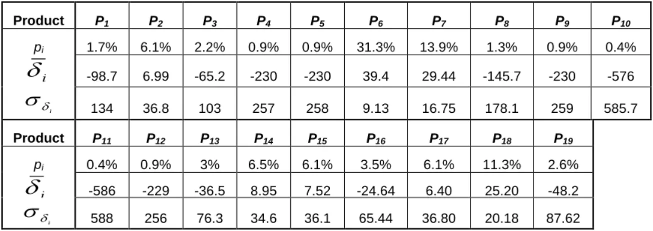
The study of a rank-change function was conducted on the basis of a vehicle assembly line on which a workstation mounts the engine selected by the final customer, who can choose between 19 engines Pi (alternate components). The engines are produced in another plant in which there is no setup time between references on the production line. The engines are then shipped to assembling plants in packages of six identical engines. Let assume that the distribution of the demand for each engine pi is that of Table 1.

Table 1 Distribution of the probability by product

Product P1 P2 P3 P4 P5 P6 P7 P8 P9 P10

pi 1.7% 6.1% 2.2% 0.9% 0.9% 31.3% 13.9% 1.3% 0.9% 0.4%

Product P11 P12 P13 P14 P15 P16 P17 P18 P19

pi 0.4% 0.9% 3% 6.5% 6.1% 3.5% 6.1% 11.3% 2.6%

We proceeded to the simulation of a randomly generated sequence of 3 billion products following the distribution of probability from Table 1. The 12,000 first components are excluded from the simulation since they represent the transient state coming before the steady state that is our interest (this transient state was willingly overestimated). The packages can hold up to six identical products. Thus the size of the batches is six. Concerning the handling of the product of rank y in sequence S1, the rule to create S2 is as follows:

- If the required product is in the stock, it is taken out of there, thus its stock level is lowered by one unit;

- Else, the production of a batch of six products is launched, and the batch is included in the stock, which level is incremented by five;

Table 2 summarizes the simulation results for each product Pi having the probability of use

pi, their average

δ

Table 2 Rank-change expectations –standard variations of rank-changes– per product

Product P1 P2 P3 P4 P5 P6 P7 P8 P9 P10 pi 1.7% 6.1% 2.2% 0.9% 0.9% 31.3% 13.9% 1.3% 0.9% 0.4% -98.7 6.99 -65.2 -230 -230 39.4 29.44 -145.7 -230 -576 134 36.8 103 257 258 9.13 16.75 178.1 259 585.7 Product P11 P12 P13 P14 P15 P16 P17 P18 P19 pi 0.4% 0.9% 3% 6.5% 6.1% 3.5% 6.1% 11.3% 2.6% -586 -229 -36.5 8.95 7.52 -24.64 6.40 25.20 -48.2 588 256 76.3 34.6 36.1 65.44 36.80 20.18 87.62

According to the notes in Figure 1, a negative value for rank-change

δ

recently arrived product is advanced regarding its positioning in the initial demand; in the example, product 10 is systematically in advance. A positive value means that the product arrived with delay compared to its initial positioning, as product 6 may illustrate. The weighted sum of average rank-changes

δ

1

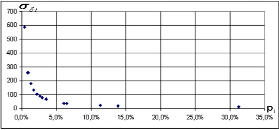
. The rank-change curves of the products are not identical: the mathematical expectation of the rank-change of products varies in the same way as their probability of use (Figure 2), whereas the standard deviations of product rank-change vary in inverse order of their use probability (Figure 3). Therefore, those products in low demand are delivered somewhat ahead of schedule, whereas the delivery of products in high demand is quite delayed.

1

In steady state, there is necessarily compensation between won and lost ranks. On a sample, the observed average (here

δ

i

δ

δ

σ

σ

Figure 2 Evolution of the mathematical expectation of rank-change of products according to their probabilities pi

Figure 3 Evolution of the standard variation of rank-change of products according to their probabilities pi

The rank-change function of a product i depends both on the number I of products (I = 1,..,I) and on the distribution of probabilities pi. Figure 4 details the occurrences of rank-change for a product with low demand, and Figure 5 is for the product with the highest demand; outlined with different scales. In the case of a product with low demand, the rank-change is essentially negative, with widely spread negative values (up until 1,000 won ranks, even 2,000 at certain points) and a very heterogeneous occurrence of values: on there is a peak for a small amount of lost ranks, then the occurrence of rank-changes decreases as the number of won ranks increases. In the case of a product with high demand, rank-changes are positive, but the number of lost ranks remains quite low though (approx. no more than 75). The occurrence of rank-changes is symmetrical to an approximate value of 40 lost ranks, with no high difference between the occurrences.

Figure 4 Curve of rank-changes for product P12 (p12 = 0.9 %;

δ

=

−

229

Figure 5 Curve of rank-changes for product P6 (p6 = 31.3 %;

δ6= 39.4

δ6= 39, 4

)

Lot-sizing creates rank-changes, which in turn can create stockout. The customer must thus form safety stocks (at the vehicle assembling plant) to avoid the side of lot-sizing on supply.

2. NEED OF A SAFETY STOCK TO COUNTER THE SIDE EFFECTS OF

RANK-CHANGES INDUCED BY THE LOT-SIZING

We shall first explain the need of a safety stock to face the lot-sizing in a deterministic universe, and then its determining factors will be analyzed.

2.1. Explanation of the need

We have seen that the probability that the delivered products match with those to assemble is very low, because of the rank-changes induced by the lot-sizing. To avoid an interruption of supply, one needs to maintain a safety stock for every complete product. These safety

i

f

δ

δ

f

stocks are fed by early products, which consequently lower the amount of products left to create the safety stock. Late products refill the safety stocks from which products where taken to ensure punctual assembly. We have seen that products with low demand are ordered (and thus delivered) somewhat in advance, but their high dispersal force the creation of safety stocks. On the contrary, the strongly demanded engines are delivered with average delay, but their dispersal minimizes the need of safety stocks.

It is important to precise that every rank-change does not systematically create an interruption of supply and, consequently, the creation of a safety stock: the supplier’s deliveries concern γ delivered batches with a lead time θ. Thus it is not sequence S2 that determines interruptions of supply but the constitution of a group of γ delivered products, while changes in this group are still possible without bearing any consequence.

2.2. Analysis of the factors determining the safety stock

In this type of case, it is not possible to obtain analytic results from the rank-change function of a reference on the basis of the multinomial distribution. Only a simulation can be performed. This procedure allows highlighting “tendencies” of the impact of certain factors, as every set of hypothesis is likely to modify the relative impact of the considered factors.

Every simulation was performed on a demand of 6 billion products, in order to empirically obtain safety stocks SSi with an insignificant stock-out probability. At the beginning of the simulation, the amount of available products was set to a value W. The first delivery is made immediately before the first product is taken. This first delivery corresponds to the θ first products of sequence S2 and the first withdrawn product corresponds to the first product of sequence S1. Each safety stock level is calculated as the difference between W and the lowest inventory level during the simulation, since W must be high enough to avoid an empty stock.

In deterministic universe, safety stocks depend on the rank-changes and on the lead time θ. The rank-changes depend in turn on the range I of products and on their probabilities pi. We will evaluate the safety stock level by a simulatory approach of the steady state. We shall study the impact of various factors on the safety stock, in a context of a lot-sizing caused by transportation constraints. First of all, we shall analyze the impact of probabilities on the safety stock. On the basis of the data in Table 1, we obtain by those simulations the following safety stock amounts (Table 3).

Table 3 Safety stocks related to rank-change Product P1 P2 P3 P4 P5 P6 P7 P8 P9 P10 pi 1.7% 6.1% 2.2% 0.9% 0.9% 31.3% 13.9% 1.3% 0.9% 0.4% SSi 5 10 6 4 4 33 17 5 4 3 Product P11 P12 P13 P14 P15 P16 P17 P18 P19 pi 0.4% 0.9% 3% 6.5% 6.1% 3.5% 6.1% 11.3% 2.6% SSi 3 5 8 11 11 8 10 16 8

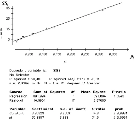
The safety stock of products varies in the same way as their probabilities (Figure 6), which was not obvious a priori. In this industrial example, an approximately linear relation can be noticed (

ρ

_ˆ

Figure 6 Evolution of the safety stock SSi according to the probabilities pi

We shall thereafter study the impact of the dispersal of probabilities on the safety stock level, on average this time. The various products can have equal probabilities: this is a case of equal probabilities of demand. They can also be extremely different, all situations are possible. We thus proceeded to new simulations, replacing the observed probabilities by distribution

p

=

p

×

k

+

b

∑

ipi . We shall outline various possible curves, descending and of exponential nature. We state that b = 0,005; it is a limit corresponding the lowest probability for a product. k is the factor for controlled decrease.

SSi

The closer it is to 1 k, the more equal probabilities of component demands are. Figure 7 illustrates the distribution of these probabilities.

Figure 7 Example of curves of probability distribution

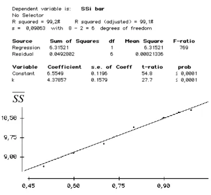
An approximately linear relation can be noticed (

ρ

ˆ

SS

Figure 8 Evolution of the average safety stock

SS

0,00 5,00 10,00 15,00 20,00 25,00 30,00 35,00 40,00 45,00 50,00 0 2 4 6 8 10 12 14 16 18 20 i pi k=0,5 k=0,7 k=0,9 k=0,99 k

SS

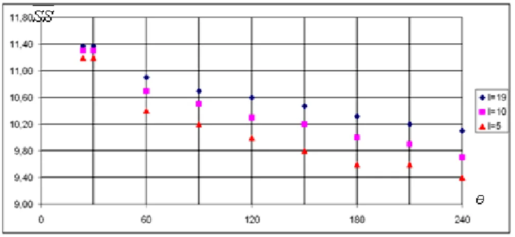
The following factor of variation corresponds to the supply periodicity θ. We proceeded to an analysis of its impact by repeating the same simulation with different values for θ. This analysis was performed using three structures of demand, with 5, 10 and 19 possible products, plus an equal probability of demand between those products (yielding the worst case for safety stock). We note that when the lead time increases, the average safety stock decreases in a fairly constant way (Figure 9).

Figure 9 Average safety stock

SS

The use of three different structures of demand allows highlighting two phenomenons. The first impression, on which we will further elaborate, is that when the variety of products increases, the average safety stock decreases, which seems logical because when the variety is lower, lot-sizing induces rank-changes of necessarily lesser importance. The second remark is that of a similarity between the variation profiles of the safety stock compared to the lead time for various values of I: the series of points for various values of I really look alike.

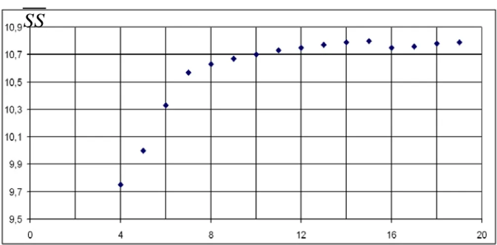
We proceed to a more in-depth analysis of the impact of variety I on the average safety stock for equal distributions, as illustrated in Figure 10. The more products, the greater the average safety stock needs to be in order to counter rank-change side effects. However, this increase is not proportional to the increase of variety: the increase is strong for values of I under 8 included, then slightly less pronounced for I between 8 and 12, the average safety stock closing in to an asymptote for I greater than 12. This means that increase of the variety of products has a strong impact on the average safety stock for I ≤ 12 in our example, but beyond those values I, adding one or several alternate components bears no consequence on the average safety stock lever (if properly calculated).

Figure 10 Average safety stock

SS

Looking more closely at the distribution of demand in our industrial case, we notice that four products have very few orders: engines 10 and 11 have a probability of 0.4% and engines 9 and 12 of 0.9%. There is neither delay nor setup cost related to a reference change on the production line. Removing these four products makes no change on the average safety stock: it is the same, whether 15 or 19 references are produced. Thus removing the offer of these four products is no advantage to either the customer (average safety stock does not decrease) or the supplier (no reference change cost).

Safety stocks are also created to counter other hazards: quality problems in a production context, variation of transportation time or modification of the firm sequence of final demand. These are explicitly excluded from the analysis, but it is obvious that the integration of a combination of disruptions leads to a mutualization of risks. The safety stock required to face multiple disruptions is thus less than the sum of all required safety stocks if the disruptions are considered separately.

We illustrate the impact of a combination of disruptions on the safety stock from an example of rank-changes caused by sizing issues at production. The analysis of this type of lot-sizing is similar to that of delivery constraints. The submitted information concerns batches between the selected unit (engine manufacturing plant) and its provider. Several technical constraints, such as limited space at line side on a station handling big components, can lead to the production scheduling in a sequence of successive batches. The difference with the previous situation (procurement) is that these batches may not concern the same

I

product, but products sharing a common specification, like containing a same component (in our case, a same crankcase used by several different engines).

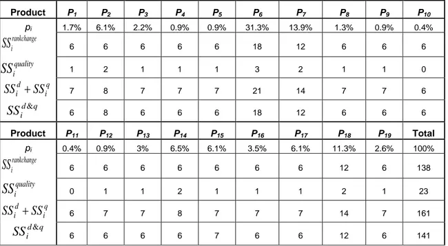
This lot-sizing is slightly more complex. On the one hand, it implies submitting information about batches of component to deliver to the supplier. But on the other hand, it leads to the creation of a second lot-sizing at the production of the designated unit, which is not homogeneous, for the batch thus created contains various products. Table 4 gives an illustration of this. We simulate the impact on the safety stock of a separate, then simultaneous integration of:

- The rank-change related to production constraints: lot-sizing of the engines by batches of 24 identical crankcases.

- Quality issues: percentage of rejection after production amounting 2%.

Once again, the safety stock is held by the customer (engine manufacturing plant) that has to own a safety stock of engines. The simultaneous integration of both disruptions allows

decreasing the safety stock required to avoid stock-out by 12.4% 161

141 161− ₌

.

Table 4 Decrease of the safety stock induced by a mutualization of disruptions

Product P1 P2 P3 P4 P5 P6 P7 P8 P9 P10 pi 1.7% 6.1% 2.2% 0.9% 0.9% 31.3% 13.9% 1.3% 0.9% 0.4% 6 6 6 6 6 18 12 6 6 6 1 2 1 1 1 3 2 1 1 0 7 8 7 7 7 21 14 7 7 6 6 8 6 6 6 18 12 6 6 6 Product P11 P12 P13 P14 P15 P16 P17 P18 P19 Total pi 0.4% 0.9% 3% 6.5% 6.1% 3.5% 6.1% 11.3% 2.6% 100% 6 6 6 6 6 6 6 12 6 138 0 1 1 2 1 1 1 2 1 23 6 7 7 8 7 7 7 14 7 161 6 6 6 6 7 6 6 12 6 141

2.3. Managerial implications

The supply chain is subjected to multiple risks. To avoid the stock shortages, the factories constitute safety stocks of the components to be assembled. When the factory can assemble on order and its supplier can produce on order, the synchronous production is

rankchange i

SS

SS

SS

SS

+

SS

SS

SS

+

SS

SS

SS

possible. When the differentiation of the components is made in the supplier's plant, it is often necessary to adapt the containers to the shapes of the products to be delivered. The batch constraints due to efficiency search in transport then oblige to constitute safety stocks even if the problem is in deterministic universe. Most of the time, the need and the importance of these stocks are not perceived because they were created to face various risks. From a managerial point of view, the existence of this kind of stock related to batching considerations is important to understand that the stocks reduction by a better control of the risks has limits. In addition, it poses the problem of the localization of the differentiation. Made in the supplier, one will have to multiply the types of containers. Made at the customer, the containers can easily be standardized but that has an impact on the design of the assembly line. This article highlights the existence of new tradeoff to be taken into account in the supply chain.

CONCLUSION

We have studied synchronization and decoupling of the control of the last two links of a supply chain dedicated to customized mass production. Taking into account lot-sizing in deterministic universe entails the creation of safety stocks. The explanatory factors of their importance were analyzed.

References

Anderson D., Pine J. (1997), Agile product development for mass customization: how to

develop and deliver products for mass customization, niche markets, JIT, build-to-order and flexible manufacturing, McGraw-Hill, New York (NY).

Giard V. (2003), Gestion de la production et des flux, Economica, Paris, 3rd ed.

Giard V., Danjou F., Boctor F. (2001a), Rank-changes in production/assembly lines: impact and analysis, Actes du 4ème Congrès International de Génie Industriel, Marseille, pp.

259-269.

Giard V., Danjou F., Boctor F. (2001b), Analyse théorique des décyclages sur lignes de production, Journal Européen des Systèmes Automatisés, Vol. 35, No. 5, pp. 623-645.

White C., Wilson R. (1977), Sequence dependent set-up times and job sequencing,