HAL Id: halshs-01062315
https://halshs.archives-ouvertes.fr/halshs-01062315
Submitted on 9 Sep 2014
HAL is a multi-disciplinary open access
archive for the deposit and dissemination of
sci-entific research documents, whether they are
pub-lished or not. The documents may come from
teaching and research institutions in France or
abroad, or from public or private research centers.
L’archive ouverte pluridisciplinaire HAL, est
destinée au dépôt et à la diffusion de documents
scientifiques de niveau recherche, publiés ou non,
émanant des établissements d’enseignement et de
recherche français ou étrangers, des laboratoires
publics ou privés.
prediction
Frédéric Ferraty, Martin Paegelow, Pascal Sarda
To cite this version:
Frédéric Ferraty, Martin Paegelow, Pascal Sarda. Polychotomous regression : application to landcover
prediction. Statistical case studies, Springer Verlag, 13 p. en ligne, 2005. �halshs-01062315�
Contents
1 Landcover Prediction 3
Fr´ed´eric Ferraty,Martin PaegelowandPascal Sarda.
1.1 Introduction . . . 3
1.2 Presentation of the data . . . 4
1.2.1 The area: the Garrotxes . . . 4
1.2.2 The data set . . . 4
1.3 The multilogit regression model . . . 6
1.4 Penalized log-likelihood estimation . . . 7
1.5 Polychotomous regression in action . . . 8
1.6 Results and interpretation . . . 9
1 Polychotomous Regression:
Application to Landcover
Prediction
Fr´ed´eric Ferraty, Martin PaegelowandPascal Sarda.
1.1
Introduction
An important field of investigation in Geography is the modelization of the evo-lution of land cover in view of analyzing the dynamics of this evoevo-lution and then to build predictive maps. This analysis is now possible with the increasing per-formance of the apparatus of measure: sattelite image, aerial photographs, ... Whereas lot of statistical methods are now available for geographical spatial data and implemented in numerous softwares, very few methods have been improved in the context of spatio-temporal data. However there is a need to develop tools for helping environmental management (for instance in view of preventing risks) and national and regional development.
In this paper, we propose to use a polychotomous regression model to modelize and to predict land cover of a given area: we show how to adapt this model in order to take into account the spatial correlation and the temporal evolution of the vegetation indexes. The land cover (map) is presented in the form of pixels, and for each pixel a value (a color) representing a kind of vegetation (from a given nomenclatura): we have several maps for different dates in the past. As a matter of fact the model allows us to predict the value of vegetation for a pixel knowing the values of this pixel and of the pixels in its neigbourhood in the past.
We study data from an area in the Pyr´en´ees mountains (south of France). These data are quite interesting for our purpose since the mediterranean mountains
knows from the end of the first half of the 19th century spectacular changes in the land covers. These changes come from the decline of the old agricultural system and the drift from the land.
The paper is organized as follows. In section 1.2, we describe more precisely the data. The polychotomous regression model for land cover prediction is presented in section 1.3. We show how to use this model for our problem and define the estimator in 1.4. Application of this model to the data is given in sections 1.5 and 1.6. Among others, we discuss how to choose the different parameters of the model (shape of the neighbourhood of a pixel, value for the smoothing parameter of the model).
1.2
Presentation of the data
1.2.1
The area: the Garrotxes
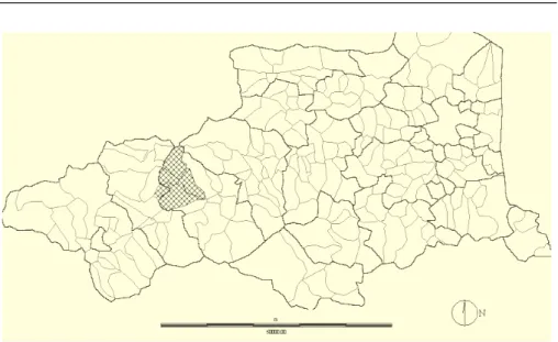
The “Garrotxes” is an aera in the south of France (Pyr´en´ees mountains). More exactly, it is localized in the department (administrative area) of Pyr´en´ees Ori-entales: see Figure 1.1 below. The type of agriculture was essentially agropas-toral traditional. Then, this area has known lot of changes in the landcover from the 19th century. Whereas agriculture has almost disapeared due to the city migration, the pastoral activity knows an increasing from the eighties. It is important for the near future to manage this pastoral activity by means of different actions on the landcover. For this, the knowledge of the evolution of the landcover is essential.
1.2.2
The data set
The data set consists in a sequence of maps of landcover for the years 1980, 1990 and 2000. The area we have studied is divided into 40401 pixels (201×201) which is a part of the Garrotxes: each pixel is a square with side of about 18 meters. For each pixel we have
1.2 Presentation of the data 5
Figure 1.1: Localization of the Garrotxes in the department of Pyr´en´ees Ori-entales.
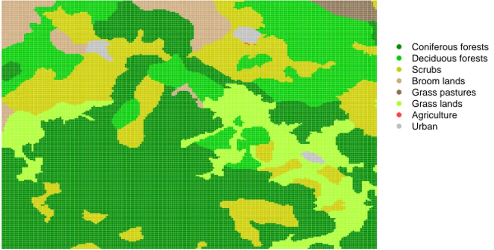
• the type of vegetation with 8 types coded from 1 to 8: 1 : “Coniferous forests”, 2 : “Deciduous forests”, 3 : “Scrubs”, 4 : “Broom lands”, 5 : “Grass pastures”, 6 : “Grasslands”, 7 : “Agriculture”, 8 : “Urban”
• several environmental variables : – elevation,
– slope, – aspect,
– type of forest management (administrative or not), – type of area (pastoral or not).
For each pixel, the environmental variables remain unchanged during the period of observation. Figure 1.2 below shows the land cover of the aera for the year 1980. Coniferous forests Deciduous forests Scrubs Broom lands Grass pastures Grass lands Agriculture Urban
Figure 1.2: Land cover for the part of Garrotxes area in 1980.
1.3
The multilogit regression model
It is quite usual to modelize a regression problem where the response is cat-egorical by a multiple logistic regression model also known as polychotomous regression model. We refer to Hosmer, Lemeshow (1989) for a description of this model and to Kooperberg, Bose, Stone (1987) for a smooth version of this model. In our context we aim at predicting the type of vegetation for a pixel at date t by the types of vegetation of this pixel and of neighbouring pixels at date t − 1: thus the model takes into account both spatial and temporal aspects. Moreover we will include in the set of explanatory variables environ-mental variables which does not depend on time. Let us note that we have
1.4 Penalized log-likelihood estimation 7
chosen a time dependence of order 1 since it allows to produce a model not too complex with a reasonable number of parameters to estimate (with respect to the number of observations). Note also that the size and the shape of the neighborhood will be essential (see below for a discussion on this topic). We give now a more formal description of the polychotomous regression model for our problem. For each pixel i, i = 1, . . . , N , let us note by Xi(t) the type
of vegetation at time t. We then define for pixel i a neighborhood, that is a set of pixels Ji. Our aim is to predict the value Xi(t) knowing the value of Xj(t −
1), j ∈ Ji, and the value of environmental variables for pixel i denoted by Yi=
(Y1
i , . . . , YiK) (independent of t). Denoting by Di(t − 1) = {Xj(t − 1), j ∈ Ji}
and by V the number of different vegetation types (8 in our case), we will predict Xi(t) by an estimation of the quantity
arg max
v=1,...,V P(Xi(t) = v|Di(t − 1), Yi) .
At first let us write
P(Xi(t) = v|Di(t − 1), Yi) = exp θ (v|Di(t − 1), Yi) PV v=1exp θ (v′|Di(t − 1), Yi) , where θ(v|Di(t − 1), Yi) = log P(Xi(t) = v|Di(t − 1), Yi) P(Xi(t) = V |Di(t − 1), Yi) .
Now, the polychotomous regression model consists in writting θ(v|Di(t− 1), Yi)
as θ(v|Di(t − 1), Yi) = αv + X x∈Di(t−1) V X l=1 βvl11[x=l]+ K X k=1 γvjYik, where δ = (α1, . . . , αV −1, β1,1, . . . , β1,Vβ2,1, . . . , β2,V, . . . , βV −1,1, . . . , βV −1,V,
γ1,1, . . . , γ1,K, . . . , γV −1,1, . . . , γV −1,K) is the vector of parameters of the model.
Note that since θ(V |Di(t − 1), Yi) = 0, we have αV = 0, βV,l = 0 for all
l= 1, . . . , V and γV,k= 0 for all k = 1, . . . , K.
1.4
Penalized log-likelihood estimation
We estimate the vectors of parameters by means of a penalized log-likelihood maximization. The log-likelihood function is given by
l(δ) = log N Y i=1 P(Zi(t)|Di(t − 1), Yi, δ) ! .
Kooperberg, Bose, Stone (1987) have shown that introducing a penalization term in the log-likelihhod function may have some computational benefits: it allows numerical stability and guarantees the existence of a finite maximum. Following their idea, we then define the penalized log-likelihood function as
lǫ(δ) = l(δ) − ǫ N X i=1 V X v=1 u2iv, where for v = 1, . . . , V uiv = θ(v|Di(t − 1), Yi, δ) − 1 V V X v′=1 θ(v′ |Di(t − 1), Yi, δ),
and ǫ is the penalization parameter. For reasonable small values of ǫ, the penalty term would not affect the value of the estimators.
For numerical maximization of the penalized log-likelihood function we use a Newton-Raphson algorithm.
1.5
Polychotomous regression in action
As pointed out above the estimators of the parameters of the model will depend on the size and on the shape of the neighborhood for pixels and on the value of the penalization parameter ǫ. For the shape of the neighborhood we choose to keep it as a square centered on the pixel. We have then to choose the (odd) number of pixels for the side of the square and the value of ǫ. The choice has been achieved through two steps namely an estimation step and a validation stepdescribed below.
• The estimation step is based on the maps from the years 1980 and 1990: it consists in calculating the estimator bδof δ for several values of the size of the neighborhood and of the penalization parameter ǫ. The computa-tion of δ is achieved by the maximizacomputa-tion of the penalized log-likelihood function defined at the previous section.
• For the validation step, we use the map for the year 2000 and compare it with the predicted map for this year using the estimator computed previously in the following way. Once the estimator bδhas been computed,
1.6 Results and interpretation 9
we estimate the probability of transition replacing the parameter by its estimator. We then obtain the quantities
b
P(Xi(t + 1) = v|Di(t), Yi), v = 1, . . . , V.
At time t + 1 (in this case t + 1 = 2000), we affect the most probable type of vegetation at pixel i, that is the value v which maximizes
n b
P(Xi(t + 1) = v|Di(t), Yi)
o
v=1,...,V .
We then keep the values of the size of the neighborhood and of ǫ which produces a map with the best percentage of well-predicted pixels (for the year 2000).
Finally we use the values selected in the last step above to produce a map for the year 2010. Concerning the implementation of such a method, all programs are written with the R language (R, 2004); maps and R sources are available on request.
1.6
Results and interpretation
To see the accuracy of our porcedure we compare the (real) map for the year 2000 with the predicted map for this year. Figure 1.3 shows this true map of land cover.
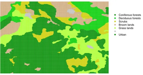
After having used the procedure as described in the previous section, we have selected a squared neighborhood of size 3 pixels and a parameter ǫ equal to 0.1. With these values we produced an estimated map (for the year 2000) shown in figure 1.4.
Table 1.1 below shows the percentage of different types of vegetation in the map of the year 2000 compared with the estimated perecentage. Table 1.1 shows that globally the predicted percentage are quite near of the real percentages. However, we have to compare the position of the vegetation types to look at the accuracy of the procedure. We consider now the percentage of missclassified pixels. The global percentage of missclassified pixels was 27.9 %. This can be seen as a quite good percentage since only 3 dates are available. Also, the performance of such a procedure can be seen by comparing figures 1.3 and 1.4 which show similar global structures. However if we look at the details
Coniferous forests Deciduous forests Scrubs Broom lands Grass pastures Grass lands Agriculture Urban
Figure 1.3: Land cover for the part of Garrotxes area in 2000.
Land cover types True percentage Estimated percentage
Coniferous forests 44.5 49.6 Deciduous forests 17.4 10.1 Scrubs 19.1 11 Broom lands 4.7 12.3 Grass pastures 12.3 16 Grasslands 0.0001 0
Table 1.1: Percentage of different vegetation types in 2000.
of missclassified pixels with respect to each type of vegetation we obtain the following table 1.2 (we retain only the types of vegetation which cover at least 1 percent of the area).
Table 1.2 shows that the results are quite different for different types of vegeta-tion: Coniferous forests, Broom lands and Grasslands are well predicted for the two firsts and quite well for the third. At the opposite, Deciduous forests and Scrubs are badly predicted (more than half of the pixels are not well predicted). This fact can be explain in two ways. At first, Deciduous forests and Scrubs
1.6 Results and interpretation 11 Coniferous forests Deciduous forests Scrubs Broom lands Grass lands Urban
Figure 1.4: Estimated land cover for the part of Garrotxes area in 2000.
Land cover types True percentage Percentage of missclassified pixels
Coniferous forests 44.5 7.1
Deciduous forests 17.4 44.8
Scrubs 19.1 65.5
Broom lands 4.7 28.1
Grasslands 12.3 18.5
Table 1.2: Percentage of missclassified pixels in 2000.
are unstable in the sense that they are submitted to random effects that our model does not take into account. For instance, into the period of ten years separating two maps a fire can transform deciduous forest into scrubs. This can explain that scrubs is the more dynamic type of vegetation. Moreover, the classification of several types of vegetation is subject to some measure of error: as a matter of fact the frontier between deciduous forests and scrubs is not so easy to determine.
As a conclusion to our study, we have seen that the polychotomous procedure introduced to predict land cover maps has given in a certain sense some quite
good results and also has shown some limitations. Stable and frequent vege-tation types have been well predicted. In the opposite, results for vegevege-tation types submitted to random changes are not so good. We see several ways to improve further studies for land cover prediction. On the geographical ground, it is important to have closer dates of measures which will lead to have a more precise idea of the dynamics. It is also important to think of defining a precise nomenclatura of vegetations. For the modelization aspects, the polychotomous regression could also be improved for instance by taking different shapes of neighborhood (rectangular, not centered in the pixel that we want to predict or with a size depending of this pixel). We can also think to integrate additional variables in order to modelize effects such as forest fires. Finally we can com-pare this procedure with other modelizations: this has been done in Paegelow, Villa, Cornez, Ferraty, Ferr´e, Sarda (2004) and in Villa, Paegelow, Cornez, Ferraty, Ferr´e, Sarda (2004) where a Geographic Information System and a neural netwok procedure have been investigated on the same data sets. The third approaches lead to quite similar reults (and similar rates of missclassified pixels). Also the same limitations have been highlighted.
Bibliography
Cardot, H., Faivre, R. and Goulard, M. (2003). Functional approaches for predicting land use with the temporal evolution of coarse resolution remote sensing data. Journal of Applied Statistics, 30, 1201-1220.
Hosmer, D. and Lemeshow, S. (1989). Applied Logistic Regression. Wiley, New York.
Kooperberg, C., Bose, S. and Stone, C.J. (1987). Partially Linear Models. Springer-Physica-Verlag, Heidelberg.
Paegelow, M., Villa, N., Cornez, L., Ferraty, F., Ferr´e, L. and Sarda, P. (2004). Mod´elisations prospectives de donn´ees g´eor´ef´erenc´ees par approches crois´ees SIG et statistiques. Application `a l’occupation du sol en milieu montagnard m´editerran´een. CyberGEO, 295, http://www.cybergeo.presse.fr.
R Development Core Team (2004). R: A language and environment for statisti-cal computing. R Foundation for Statistical Computing, Vienna, Austria. Villa, N., Paegelow, M., Cornez, L., Ferraty, F., Ferr´e, L. and Sarda, P. (2004). Various approaches to predicting land cover in Mediterranean mountain areas. Preprint