Revue internationale de géomatique – n° 1/2013, 39-70
Agro-environmental risk evaluation
by a spatialised multi-criteria modelling
combined with the PIXAL method
Francis Macary
1, Odile Leccia
1, Juscelino Almeida Dias
2Soizic Morin
3, José-Miguel Sanchez-Pérez
4, 51.Irstea, UR ADBX, 50 av. de Verdun, 3612 Gazinet Cestas, France 2. Université de Paris-Dauphine, LAMSADE
Place du Mal De Lattre de Tassigny, 75 775 Paris Cedex 16, France 3.Irstea, UR REBX, 50 av. de Verdun, 33612 Gazinet Cestas, France 4. Université de Toulouse, INPT, UPS
EcoLab (Laboratoire écologie fonctionnelle et environnement), ENSAT Avenue de l’Agrobiopôle, 31326 Castanet-Tolosan, France
5. CNRS, EcoLab, 31326 Castanet-Tolosan, France
ABSTRACT.The degradation of water quality due to agricultural inputs is now a major problem in all regions where fertilizers and pesticides have been widely used for best yields. In order to improve the situation in the field, public agricultural and environmental services need to assess the agro-environmental risks at different spatial levels in order to apply the appropriate measures. We researched the assessment of these risks by studying current practices at different spatial scales. This was carried out in the Coteaux de Gascogne area of southwest France, using first, ELECTRE TRI-C multi-criteria spatial modelling combined with ArcGIS ®, on a small experimental watershed (3 km²); then AZOTOPIXAL method, which includes both remote sensing and GIS on a 1,150 km² watershed. We identified a functional relationship between these two decision aiding methods, and then attempted to validate the results by taking measurements of nitrogen concentration in surface water.
RÉSUMÉ. La dégradation de la qualité des eaux par les intrants utilisés en agriculture est devenue un problème majeur dans toutes les régions où les fertilisants et les produits phytosanitaires ont été largement utilisés pour augmenter les rendements. Afin de mettre fin à cette situation et d’appliquer des mesures adaptées au terrain, les gestionnaires des services publics de l’agriculture et de l’environnement ont besoin d’informations sur les risques agro-environnementaux à différents niveaux de l’organisation spatiale. Nous avons mené des recherches sur l’appréciation de ces risques en effectuant une évaluation à différentes échelles spatiales en fonction des pratiques. Ainsi, nous avons mis en œuvre deux méthodes dans les coteaux de Gascogne (sud-ouest de la France). D’abord, nous avons appliqué une modélisation multicritère avec la méthode ELECTRE TRI-C combinée à un SIG ArcGIS ®, dans un petit bassin versant expérimental (3 km2). Ensuite, nous avons utilisé la méthode AZOTOPIXAL combinant simultanément télédétection et SIG dans le grand bassin versant
englobant de 1 150 km2. Nous avons développé une relation fonctionnelle entre ces deux méthodes d’aide à la décision. Ensuite, nous avons tenté de valider les résultats obtenus à partir de mesures de la concentration en nitrates dans les eaux de surface.
KEYWORDS: agricultural practices, ELECTRE TRI-C method, environmental risks, GIS, multi-criteria decision aiding, nitrogen, AZOTOPIXAL method, remote sensing, scale changing.
MOTS-CLÉS : pratiques agricoles, méthode ELECTRE TRI-C, risques environnementaux, SIG,
aide multicritère à la décision, azote, méthode AZOTOPIXAL, télédétection, changement d’échelle.
DOI:10.3166/RIG.23.39-70 © 2013 Lavoisier
1. Introduction
Over the last five decades, certain areas have seen a development of intensive agricultural practices. As a result of this, the widespread use of fertilisers and pesticides has become a cause for environmental concern, posing a risk to surface and groundwater (OECD, 1998). At the same time, the increased use of products containing nitrogen has greatly increased crop yields (Henin, 1980; Sebillotte, 1992; 1994; Turpin, 1997).
Increased sales of nitrogen fertilizer, along with the intensification of farming practices and the changing layout of farmland, have significantly modified the nitrogen cycle. Agricultural ecosystems – including surface and groundwater – have become overloaded with nitrates (Probst, 1985; Sanchez-Pérez et al., 2003; Perrin et
al., 2006; Birgand et al., 2007). Common agricultural policy has meant that farmers
have maintained a level of production which far exceeds the needs of the population, and the export of farm produce has been increased without any thought to the resulting impact on the environment.
In response to this situation, the European Union created the Water Framework Directive (WFD), aimed at protecting the ecological status of fresh surface and groundwater within Europe (WFD/2000/60). This policy sets out legal and regulatory specifications for member states to achieve a “good” level of ecological and chemical cleanliness for all natural aquatic environments by 2015. Agriculture is one of the considerations in this new directive. In France, agriculture and the environment have their own dedicated ministries, who in turn control regional agencies such as local healthcare authorities and water supply bodies. At regional level, the activities carried out by these organisations are managed by the Prefect (Préfet) (a senior government representative).
The facilities most affected by these new regulations on excess pesticides and nitrogen are the pumping stations that provide drinking water to the local population. European standards impose a maximum concentration of 0.1 µg/L for any single type of pesticide molecule in water destined for public consumption, and a maximum total concentration of 0.5µg/L where multiple molecules are present
(EC, 1998). For nitrates, the limit is set at 50 mg NO3/L. Untreated water for
consumption by humans and animals is obtained directly from groundwater through pumping stations.
Water pollution has become a key issue for water managers, as many stations have been closed down due to their chemical levels significantly exceeding legal limits. These high concentrations of nitrogen and pesticide molecules are largely due to intensive farming.
Despite certain farmers voluntarily adopting improved methods since 1992 – the third major reform of the European common agricultural policy (Weyerbrock, 1998) – the effects have been negligible. The adoption of these new practices has simply been spread too thinly.
European governments have implemented a variety of measures to reduce the concentration of pollutants more effectively. In France, the agriculture and environment ministries enacted Decree n° 2001-34 (MATE, 2001), which applied the specifications of the European Nitrate Directive (CE, 2001). This decree was later superseded by Decree n°. 2007-397 (MEDD, 2007). These new regulations were essentially intended to reduce the transfer of nitrates from cattle farms to water, and to stop them spreading to vulnerable areas.
The 2007 French environment summit, or “Grenelle de l’environnement” (MEDDTL, 2007) saw the introduction of a new environmental protection law (MEDDTL, 2010). The French Agriculture Ministry promoted contracts between the State and farmers who receive subsidies, provided to develop Best Management Practices (BMPs) and Best Environmental Practices (BEPs) (Lafitte and Cravero, 2010). BEPs may include measures aimed at the reduction of agricultural pressure affecting water (nitrates, pesticides, etc.) or reducing the effects of this pressure (buffer zones, limiting excess nitrates, etc).
Two distinct approaches can therefore be identified. The first involves changing the production methods themselves, through moves towards organic farming, input/output optimization (Kirchrnann et al., 2005). An essential part in this process is to convince farmers of the benefits of more environmentally-friendly methods.
The second approach aims to reduce the impact of farming pressures through BMPs, such as extending time between crop rotations, and implementing crop catching, crop residue management, and vegetative strips. It can also make use of BEPs such as retention ponds and riparian zones (FAO, 1994; Misra et al., 1996; CORPEN, 1997; Schmitt et al., 1999; Gril and Lacas, 2004; Carluer et al., 2009).
To make the most effective use of these new measures, financial incentives need to be focused on areas with the highest risk of pollutant transfer, and are thus designed with the specific aim of reducing pollution of river waters. Limits aimed at protecting water pumping zones also need to be precisely defined. The implementation of these measures requires well-managed environmental engineering.
In order to assess the dominant processes responsible for poor water quality, we need to take into account the relationships between landscapes, land use, and the impact of anthropogenic pressure on natural cycles. Over the last 20 years, simulation tools have been developed, which analyse the quality of surface and groundwater, taking into account data from agronomical, hydrological, and ecological sources.
Water quality assessment models have previously provided a significant contribution to the analysis and understanding of non-point source pollution, as measured in rivers, aquifers, and reservoirs (Arnold, 1998; Beaujouan et al., 2002; Bioteau et al., 2002; Gomez et al., 2003; Oehler et al., 2009; Ferrant et al., 2011; Oeuring et al., 2011).
These tools are able to simulate potential changes in both of the quantity and quality of surface and groundwater, according to human pressure and natural dynamics. However, these types of models require a large number of parameters and data. Environmental managers are often unable to use them because they are simply too complicated, and the necessary data can rarely be obtained. In addition to this, qualitative data, such as that concerning BEPs, are incompatible with this modelling method.
Our first task was to develop our own method using BEP and BMP scenarios, which would in turn allow us to take into account qualitative information when carrying out agro-environmental risk assessments. This approach provides managers of agricultural and environmental agencies with effective, easy-to-use decision support tools.
The risk of water contamination by agricultural chemicals is assessed using factors that fall into two categories. The first category takes into account water vulnerability, i.e. the combination of slopes, soil types, and the proximity of farmland to streams and rivers. Certain BEPs can only be assessed at a local scale. The second category of factors covers agricultural pressure (nitrogen, pesticides, etc).
We applied two methods, each adapted for a different spatial scale. For small watersheds (less than 10 km²), we used a multi-criteria decision aiding method (MCDA) called ELECTRE TRI-C, coupled with a GIS (ArcGis®). This method needs investigation in the field.
For large watersheds, (several hundreds or thousands of km²) we used a combination of remote sensing and GIS. We carried out supervised classification of satellite images (Landsat 5TM), using a GIS to give us land use information.
The second step in the process was to link these two methods, and to use locally-obtained MCDA information to optimise the remote sensing/GIS method. This new combined use of methods is the main topic of this paper.
2. Materials and methods 2.1. Study site
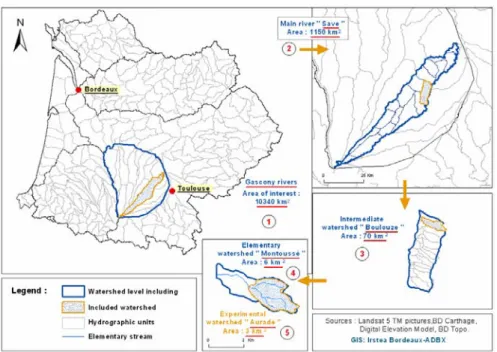
Our research was carried out in the Gascony region in southwest France (Figure 1). Figure 1 illustrates the layout of the Adour-Garonne hydrographical network, including the main tributaries leading to the Garonne River (1). It shows the large Save watershed (2), a hydrographical zone contained within the Save watershed, called the Boulouze (3), an elementary watershed, the Montoussé (4), and the small Auradé watershed (5), which was used as the example for our research. The different scales for studying agro-environmental risks are shown on this map.
The aim of our model is to provide environmental managers and stakeholders with results for each of these different scales.
Figure 1. An overview of the scaling change issue and location of the study site
With a surface area of 10,340 km², the Gascony region is within the watershed of both the Adour and Garonne, and is drained by 17 rivers. The rivers in Gascony are all left tributaries of the Garonne, which is located between the Pyrenees and the Atlantic Ocean. All of these rivers begin on the Lannemezan plateau. Some of these watersheds, such as the Save (1,150 km²), cover several thousand square kilometers.
Between 1985 and 2004, the mean annual rainfall was in the region of 700 mm, with evapotranspiration of 820 mm. The rivers in question are subject to a rain-driven hydrological regime. Low flow period occurs during the summer season (between July and September). The geological substratum is essentially impermeable, favouring surface and subsurface runoff, and the transfer of contaminants into streams.
A great deal of intensive farming is carried out in the region, with the main crops being cereals, sunflower, soya, rapeseed and maize. Water from nearby rivers is often used for irrigation. Parcels of land located on slopes generally have short crop rotations of around two or three years. A lot of chemicals, such as nitrogen and pesticides, are used on these hillside plots to boost yields.
The quantities in which these substances are used give a good illustration of the levels of intensive farming in a given area.
In addition to this, many parcels are large when compared to the regional average, often covering over ten hectares. This is because many forests, hedges, and grasslands were removed some fifty years ago as part of a process of land consolidation, following a mass rural exodus.The increasing use of large machinery has also contributed to the size of the parcels. Intensification of farming practices has led to a very real decrease in the quality of surface water (Perrin et al., 2006).
2.2. General conceptual model combining two methods for varying spatial scales
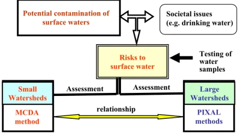
Our multi-scale assessment of agro-environmental risks took into account both the vulnerability of surface water and agricultural pressure. By combining these two elements, we were able to determine the potential contamination of streams and rivers. Where this kind of contamination is likely to affect drinking water pumping stations, it represents a territorial surface water risk (CORPEN, 2006).
The general conceptual model is shown below (Figure 2). Assessments were carried out at the “small” watershed scale using an MCDA method. For larger watersheds, we employed a PIXAL method. The term “PIXAL” is a generic term given to spatial agri-environmental risk assessment. Initial calculations are made using remote sensing data (Landsat TM: 30m x 30m). Values are then aggregated at different watershed levels. Where agricultural pressure is caused by nitrogen, the method is referred to as AZOTOPIXAL (“azote” being the French word for nitrogen). For pesticide contaminants, we call the approach PHYTOPIXAL (from “phytosanitaire”: a French word relating to these chemical products).
Figure 2. General conceptual model combining two methods
The two methods share the same overall approach. The main criteria are the same, but we will see in sections 2.3 and 2.4 that the parameters are different.
For smaller watersheds, we are able to add qualitative criteria such as BEPs, which allow physical phenomena to be taken into account. A smaller scale also means that indicators can be more easily validated for farming parcels. We carried out this validation for the MCDA method, which in turn allowed us to improve the PIXAL methods we used on larger areas.
2.3. Risk assessment for a small area, through the modelling of a combined multi-criteria decision aiding method and GIS.
Decision support can be used in a wide range of contexts, including urban and regional planning, transport, management of water resources, and environmental management. This approach began in the late 60s, when researchers recognised the need to overcome the limitations of cost-benefit analyses and linear programming approaches, thus taking into account many conflicting factors.
Multi-criteria Decision Aiding (MCDA) methods, or Multi-criteria Decision Analysis methods were developed in the 1970’s (Roy, 1968), and have been used in a wide variety of contexts (Schärlig, 1985, 1996; Roy and Bouyssou, 1993; Maystre
et al., 1994). Starting in the early 1980s, they have also been successfully applied to
environmental management issues (Simos, 1990).
They can generally provide an effective insight into problems (Laaribi, 2000), where: Risks to surface water Testing of water samples Small
Watersheds Watersheds Large
MCDA method PIXAL methods relationship Assessment Assessment Potential contamination of
– Multiple quantitative and qualitative criteria are considered, – Criteria are often heterogeneous,
– Criteria are generally conflicting,
– Criteria are generally considered of unequal importance.
MCDA approaches help decision-makers who have to deal with multiple – often contradictory – points of view. Using these methods, decisions can be both modelled and formalised.
More recently, their use has been further developed to incorporate spatial information systems. Malczewski (2006) carried out an extensive review of existing literature on the combined use of MCDAs and GIS’s. This kind of integrated approach is mentioned in a large number of scientific papers (Janssen and Rietveld, 1990; Joerin et al., 2000; Laaribi, 2000; Chakhar and Mousseau, 2008).
Integration of these methods is particularly useful for agro-environmental studies, because it allows both quantitative and qualitative data to be taken into account, enabling simulations to be better tailored to the specific needs of stakeholders, policy makers, and experts. This combination has been used in a variety of previous projects, notably in irrigation water management (Tiwari et al., 1999; Chen et al., 2010; Reshmidevi et al., 2010), to select the best agricultural areas for sewage sludge amendment (Passuello et al., 2012), to develop land suitability for agriculture (Mendras and Delali, 2012), to assess erosion risk zoning (Macary et al., 2010b), and to apply European nitrate reduction policies (Fealy et al., 2010).
Given all of these advantages, we decided to use a MCDA/GIS combination for our own project, involving the creation of a decision aiding tool for water managers in the Adour-Garonne basin. The method was tested on the smaller Auradé watershed (Figure 1).
Terminology:
– Action “a” is the representation of the element which contributes to the decision, e.g. each farming parcel in the watershed where farmers manage land use and agricultural or environmental practices.
– Criterion “g” is a judgement factor with which we measure and estimate the performance of the parcels in terms of surface water contamination risk.
For each criterion, several values, called performance values, are proposed. The highest performance is associated with the strongest risk of pesticide transfer. gj (a)
is the evaluation or performance of the action “a” depending on criterion “j”. The role of the different criteria is modelled by using the weights of the criteria and, where applicable, preference, indifference and veto thresholds.
– Multi-criteria evaluation consists of measuring the parcels’ performance with regard to the criteria, using the MCDA method. The table resulting from these evaluations is called the performance matrix.
There are several types of multi-criteria problem (selection, description, classification, sorting), which need to be effectively sorted. The aim of this sorting process is to assign actions to a set of categories, calculated based on multiple criteria. This allocation was carried out using the ELECTRE TRI-C method.
Each category must be pre-defined before receiving these actions (agricultural parcels in this case), which will/may be processed in the same way. They are characterised by a benchmark action which sets the relevant transfer risk level. When applied to decision-making, the categories are ranked in order of risk.
The model prototype used for our project was developed by Almeida-Dias et al. (2010). It was modified from the previous version of the ELECTRE TRI method (Mousseau et al., 2000), in which each result category had pre-defined boundaries. With the ELECTE TRI-C method, these categories are set using benchmark values, which give a more relevant display of risk levels. Each category needs to be defined before actions can be assigned to it (in this case, farming parcels). These actions may or may not be processed in the same way.
The Assignment procedure sorts the parcels into 5 categories of risk level: Very High/High/Intermediate/Low/Very Low (or No Risk), because this is a commonly-used categorisation method for agro-environmental studies, especially when dealing with risk levels.
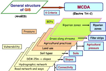
In 2009, the Auradé watershed included 83 farming parcels (actions). We defined six different criteria for the multi-criteria modelling process, based on their relevance to nitrogen transfers and information availability.
– First group: Vulnerability of surface water
- Effect of combination of slopes and homogeneous portions for each farming parcels: this is a quantitative criterion,
- Connectivity between the farming parcels and the streams: qualitative criterion,
- Soil types: qualitative criterion.
– Second group: Agricultural pressure (land use and nitrogen application in this paper) is a quantitative criterion.
– Third group: Regulation of the transfer of contaminants into surface waters - Vegetative Filter Strips (VFS) between parcels and streams: qualitative criterion,
Figure 3. Different criteria used and relations between GIS and MCDA The higher the score for each criterion, the higher the risk level
The current article is concerned with showing how we combined the MCDA and PIXAL methods, and in particular how we applied this combination to varying scales. We will therefore only provide a brief outline of the methods themselves. The implementation of the two methods in question has already been described in detail by Macary et al. (2006, 2007, 2010, and 2012).
2.3.1. Modelling the set of criteria in the MCDA method
A brief overview of the performance values used for criteria modelling.
Details of MCDA scores implemented for each criterion relating to the farming parcels in the Auradé watershed were provided in previous papers (Macary et al., 2012). These values were based on field observations.
Criterion g1 - Combination of slopes and the surface area of parcels
Slopes are an important consideration in agro-environmental risk assessment, because they affect surface runoff and thus the potential transfer of contaminants. The performance values take into account both the surface area and the slope of a parcel when calculating its risk level. We included the surface area in this criterion because of its importance to the whole calculation process. It also allows the “slope” value to be refined, because an average slope value by itself makes no sense.
(ArcGIS)
General structure of GISGIS
6 Criteria (Electre Tri-C)
MCDA
MCDA
(ArcGIS) General structure of GISGIS (ArcGIS) General structure of GISGIS General structure of GISGIS6 Criteria (Electre Tri-C)
MCDA
MCDA
6 Criteria (Electre Tri-C)
6 Criteria (Electre Tri-C)
MCDA
MCDA
MCDA
MCDA
MCDA
MCDA
Road network and ways Road network and ways
Hydrographic network Hydrographic network DEM 25m ⇒ slopes DEM 25m ⇒ slopes Soil types Land use Agricultural practices Soil types Land use Agricultural practices Vulnerability Vulnerability Pressure Pressure
Grass along streams Riparian zones BEPs BEPs Vulnerability Vulnerability Pressure Pressure
Grass along streams Riparian zones BEPs
BEPs
Grass along streams Grass along streams
Riparian zones Riparian zones BEPs BEPs Connectivity Slopes Agricultural pressure Soils Riparian zones Filter strips Connectivity Connectivity Slopes Slopes Agricultural pressure Soils Soils Riparian zones Riparian zones Filter strips Filter strips
We calculated this performance with the GIS, on the basis of a Digital Elevation Model (DEM) at 25 m restored to a precision of 10 m; each parcel was broken down into polygons u of uniform slope Pu (% of slope) and surface of polygons Su (m2).
We attributed the performance of the criterion g1 for a farming parcel, by calculating: ∑(Pu x Su).
This combination takes into account the surface area of a farming parcel in a criterion, which affects its contribution to contaminant transfer. This is a quantitative criterion.
Criterion g2 - Soil type
The flow mode of contaminants is influenced by the soil types (Macary et al., 2011). We selected four groups of soils from a set of twelve different soils determined by SOL CONSEIL-ECOLAB in 2006: A (Epileptic Cambisols-Rendzic-Leptosols (<50 cm); B (Calcaric-Cambisols > 50 cm); C (Cambisols-Luvisols); D (Fluvisols).
The scores in each parcel consider the soil types and their corresponding surface area. They were established as follows:
Soil score = (%S1 A*8 + %S2 B*4 + %S3 C*2 + %S4 D*1) / 100 (1) Sx represents the area of each type of soil per parcel.
Criterion g3 - Connectivity of each agricultural parcel to the stream
The advantage of the MCDA method is that it allows us to note qualitative elements previously observed on the watershed. as follows:
– Very high connectivity = 9
(The whole upstream edge of a parcel directly borders the stream, with some drains), – High connectivity = 8 and 6
(8: the whole upstream edge of a parcel directly borders a stream, without drains) (6: part of the edge of a parcel directly borders a stream),
– Intermediate = 5 (Talwegs and ditches) – Weak = 3 (Roads and public footpaths) – Very weak = 1 (Little or no connectivity)
Criterion g4 - Vegetative Filter Strips effects (VFS)
The VFS represents a vegetative strip used along streams in the lower parts of parcels, decreasing the transfer of soluble contaminants to the stream. However, the effectiveness of this solution depends on its width and serviceability classified in the field as follows: width “l” was appreciated in a scale between 0 and l > 9 m; serviceability was classified either as bad or good. Performance resulting from the intersection of notation is included in the range of values: [0 – 15].
Criterion g5 - Riparian Zone (RZ)
A riparian zone is a wooded area along the side of a stream. A good RZ decreases contaminant transfer and also improves the protection of streams.
The effectiveness of this type of zone depends on the density of its vegetation. These zones were scored as follows: 10 for riparian zone in [0 -10 [; 9 for RZ in [10 -25 [; 7 for RZ in [25 -50 [; 5 for RZ in [50 -75 [; 3 for RZ in [75 -100 [; 2 for RZ = 100% and 0 when land parcel is not along the stream.
Criterion g6 - Agricultural pressure: nitrogen inputs
We characterised the agricultural pressure according to nitrogen, pesticides and land use regarding erosion risks. In this paper, we only consider the nitrogen inputs. We took into account the total input Q on a crop for a year, modulated by the number of inputs Ni. This is particularly relevant for risk levels, because of the potential runoff after they are applied. Following tests, we decided to use this rule: Q = 100% when Ni =1; Q = 85% when Ni =2; Q = 75% when Ni =3; Q = 70% when Ni ≥ 4. Input values came from field surveys (Auradé Farmers Association) for each crop in agricultural parcels. The scale of raw values is from 0 to 300 kg/ha, before the modulating coefficient is applied.
Performance of the benchmark parcels for the five categories of risk levels
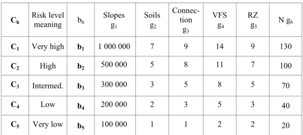
Table 1 shows the performance of the benchmark parcels, for the five categories of risk levels, based on expert judgement.
Table 1. Performance of benchmark parcels, for the 5 categories
Ch Risk level meaning bh Slopes g 1 Soils g2 Connec-tion g3 VFS g4 RZ g5 N g6 C1 Very high b1 1 000 000 7 9 14 9 130 C2 High b2 500 000 5 8 11 7 100 C3 Intermed. b3 300 000 3 5 8 5 70 C4 Low b4 200 000 2 3 5 3 40 C5 Very low b5 100 000 1 1 2 2 20
Note: Ch: Category of risk level, bh: Performance of benchmark parcels by criterion, for each
risk category.
We defined five risk levels, which is common practice among public environmental institutions in Europe (§ 2.3). We also chose to rank benchmarks B1
to B5 with decreasing values for each criterion. This allowed us to remain coherent with a ranking system used on a previous erosion study with the Electre III model (Macary et al., 2010).
The system used for that project placed farming parcels of interest to environmental managers in the top category, as they required priority analysis and re-meditation.
2.3.2. Relationship between MCDA method and GIS
The Electre method was combined with the GIS, but not directly integrated. We used GIS to calculate the performance values of farming parcels for each criterion, which were then implemented into the performance matrix. Following modelling with the MCDA method, the GIS is used to show results. With certain GIS applications, it would be difficult (or impossible in some cases) to take into account certain criteria, notably vegetative filter strip effects and riparian zones. The reason for this is that vectors (partial surface area), rather than raster cells (whole surface area) are used for each parcel. Using this method, we are able to ensure optimum performance for both systems, and data can be readily transferred between them.
2.3.3. Modelling the weights of criteria
Different criteria have varying levels of influence on the risk of contaminant transfer. Because of this, the values need to be weighted within the model. The numerical values assigned to these weightings were obtained using SRF (Simos-Roy-Figueira) software (Figueira and Roy, 2002), with the help of expert agronomists in ranking criteria based on their importance in physical processes, and then using software with a “card game” approach (Table 2).
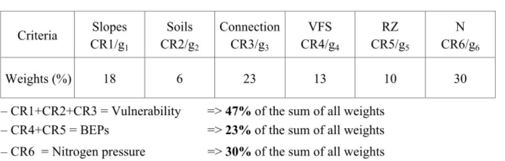
Table 2 shows the final results of the weighting. Surface water vulnerability criteria receive a weighting of 47%, nitrogen pressure 30%, and the two BEPs “vulnerability regulators”: 23%.
Table 2. Weighting of criteria
– CR1+CR2+CR3 = Vulnerability => 47% of the sum of all weights – CR4+CR5 = BEPs => 23% of the sum of all weights – CR6 = Nitrogen pressure => 30% of the sum of all weights
Criteria Slopes CR1/g1 Soils CR2/g2 Connection CR3/g3 VFS CR4/g4 RZ CR5/g5 N CR6/g6 Weights (%) 18 6 23 13 10 30
In order to account for the imprecise nature of some data, we also introduced the notion of thresholds to the model. We established three different thresholds:
Indifference (q), Preference (p), and Veto (v). This last threshold only applies to the criterion g6. The thresholds are considered as linear functions of performance gj (a) and are calculated as follows: threshold (gj (a)) = α x gj(a) + β. (the analyst must specify the value of both coefficients α and β for each criterion and for each threshold.
The Electre Tri-C assignment results are based on the outranking credibility indices, denoted σ (a, bt), (Almeida-Dias et al., 2010) which are compared to a chosen credibility level, denoted λ. This level is a minimum degree of credibility which is considered or judged necessary by expert agronomists in order to validate (or not) the statement “a outranks b” (meaning that a is at least as good as b) taking all the criteria from F into account.
In general, this minimum credibility level has a value within the range [0.5-1], and can be roughly interpreted as a majority level, as in the voting theory. For this project, we set the minimum degree of credibility (λ) at a value of 0.7 (based on our criteria weighting) which is considered necessary in validating or refusing the assignment of a farming parcel within a particular category.
2.4. The PIXAL multi-scale risk assessment methods, using remote sensing and GIS
In the past, a variety of methods have been used to deal with the problem of scale change, which is a key consideration for geographers and agronomists working at different scales, e.g. with nested watersheds. There are many different type of scale change, including:
– Creating specific agro-environmental indicators for the data needed at each scale: parcels, farms, watersheds, and administrative units.
– Aggregation and disaggregation. These approaches were applied by Blöschl and Sivapalan (1995). Disaggregation is used to determine the behaviour of a particular component, based on the behaviour of the whole entity.
Aggregation works by taking separate elements and combining them to form a whole. Indicators take raw data and convert them to a synthetic format.
A Spatial Reference Object (SRO) can be used by environmental managers and local stakeholders for each of the different scales.
The aggregation is then carried out mathematically, separately taking into account the data for each scale. Spatial information is thus displayed in a format that can be easily read and interpreted.
The accuracy of the spatial method is governed by the levels of spatial organisation. Generally speaking, the smaller the geographical scale, the more
accurate the information, as more data is available. Information obtained at these smaller scales can then be used to improve the accuracy of data applied to other levels of organisation.
With this in mind, we developed a spatial risk assessment method, aggregated at different spatial scales. Our PIXAL methods – AZOTOPIXAL for nitrogen in this paper – are suitable for use in other regions where surface waters are exposed to different contaminants. Our approach is based on a combination of complex and spatialised agro-environmental indicators, taking into account both the vulnerability of surface water and agricultural pressure.
2.4.1. AZOTOPIXAL method
We first established the risk of pollutant transfer using our own SRO, a 30m x 30m Landsat image. This image was then aggregated to include different levels of spatial organisation, ranging from small agricultural watersheds, to the larger scale of the surrounding watershed. The method was developed and tested in the Gascony region (Figure 4).
We had to exclude certain agricultural factors, because we could not obtain suitably discriminating data (e.g. geological substratums). The final factors chosen fell into two groups: natural environment (relating to surface water vulnerability) and agricultural pressure. We may note here that, unlike the MCDA approach in the small watershed, the AZOTOPIXAL method uses rasters to calculate risk levels, whose size is superior to a VFS and a RZ. This explains why VFS's and RZs cannot be taken into account. A quantitative measurement of this type would require remote sensing images with a resolution of one to five square metres. However, qualitative data regarding the effectiveness of VFS and RZ would be impossible without on-site checks by an expert.
The first group includes slopes, soil types, and connectivity with streams. The vulnerability indicator for the method is the sum of these three values. This value was selected following a number of tests using multiplication, which resulted in too much importance being given to the vulnerability value in the risk assessment (Figure 4).
The second group covers the use of contaminants (nitrogen in this paper). These data come from land use information and agricultural practices. Land use information was obtained through remote sensing (supervised classification of three satellite images by our team using Erdas Imagine®). We collected information on farming methods through interviews with farmers and their advisors.
Agricultural inputs were added directly at pixel level (in this case nitrogen doses by crop) on the GIS, taking into account the number of inputs (§ 2.4.2.3).
Our first step (Figure 4) was to calculate contamination risks, firstly at pixel level, by multiplying together vulnerability and agricultural pressure values. The choice of sign in this case is quite obvious: if pressure is zero (vulnerability could be
very low but never zero) the risk level for a particular pollutant must be zero, e.g. no fertilization applied.
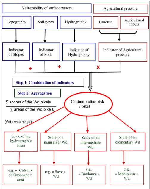
Figure 4. Overall structure of the AZOTOPIXAL method and its different scales of results (Wd: watershed)
(Wd : watershed) e.g. « Coteaux de Gascogne » area e.g. « Save » Wd e.g. « Montoussé » Wd Scale of a main river Wd Scale of an intermediate Wd Scale of an elementary Wd Scale of the hydrographic basin e.g. « Boulouze » Wd Step 2: Aggregation Contamination risk / pixel ∑ scores of the Wd pixels
∑ areas of the Wd pixels
+
x
Indicator of Agricultural pressure Vulnerability of surface waters
Agricultural inputs Agricultural pressure Landuse
+
Soil types Indicator of Soils Topography Indicator of Slopes Hydrography Indicator of HydrographyThe second stage involved aggregating contamination risk values at different spatial levels (watersheds in this case). This was achieved by calculating average values based on the surface area of the watershed. The level of aggregation depends on the area chosen by the public managers of agriculture and the environment, and the area in which water needs to be protected.
This information provides adequate scope for scale changing. Data were gathered over the full area at the smallest scale, allowing for a more precise description.
The general flowchart of the method is showed in the Figure 4.
The application of the method in the Coteaux de Gascogne area (map on Figure 1) shows how the risk assessment can be carried out for a watershed of some km2,
right up to a hydrographic basin covering several thousand square kilometres.
2.4.2. Indicator scores
2.4.2.1. Slope
We used the DEM at a resolution of 25 metres, extrapolated to a 30-metre resolution, to obtain the same spatial resolution as that of the satellite image.
We retained seven classes of slope adapted to the surface runoff < 2%; 2 to 5%; 5 to 10%; 10 to 15% to 20%; 20% to 25%; > 25%. In this area, crops are mainly grown on farmland with slopes of less than 15%. Beyond this value, we found mainly grasslands. In this study, scores from 1 to 11 were used for increasing classes of slope.
2.4.2.2. Soil types
We used the same 4 categories as those determined for the small Auradé watershed. A (Epileptic Cambisols-Rendzic-Leptosols < 50 cm): 8; B (Calcaric-Cambisols > 50 cm): 4; C ((Calcaric-Cambisols-Luvisols): 2; D (Fluvisols): 1.
2.4.2.3. Distance to water courses
Unlike the MCDA method, in which we carried out a qualitative appreciation of the connectivity, with the AZOTOPIXAL method, we use the buffer function of the GIS to determine the distance between each pixel with the watercourse. Distances were multiple of 30m (width of the satellite image pixel). We considered 5 classes: < 30m; 30 to 60; 60 to 90; 90 to 120; > 120m. Before adapting these values, we carried out different tests. When a different class was used 120 to 150m, we observed many intersections of buffer zones, in close proximity to water courses when watercourses are near.
2.4.2.4. Nitrogen inputs
We also used the values from Auradé and other watersheds for different crops unrepresented in this small area. We used the same coefficients to modulate inputted figures. We applied a value of 65 kg/ha of nitrogen for grassland, because this is a value usually considered in the same conditions.
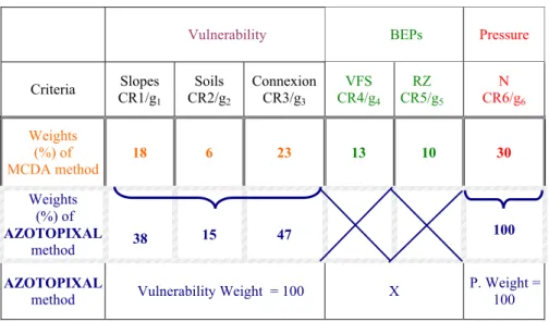
2.4.2.5. Indicators weighting
At the beginning of development of the method, no differential weighting was imposed between the scores. But after the multi-criteria modelling, we integrated weights for the indicators of vulnerability without the BEPs only, because remote sensing is not able to take them into account. These weights come from an extrapolation of the MCDA weights for the vulnerability criteria. The AZOTOPIXAL method initially adds together weighted vulnerability indicators, and then multiplies vulnerability by pressure, both of which have a weighting of 100.
Table 3 shows weights following the two methods, and how weightings are calculated for the AZOTOPIXAL and MCDA methods.
Table 3. Weighting relationships between MCDA and AZOTOPIXAL methods
Vulnerability BEPs Pressure
Criteria CR1/gSlopes 1 Soils CR2/g2 Connexion CR3/g3 VFS CR4/g4 RZ CR5/g5 N CR6/g6 Weights (%) of MCDA method 18 6 23 13 10 30 Weights (%) of AZOTOPIXAL method 38 15 47 100 AZOTOPIXAL
method Vulnerability Weight = 100 X P. Weight = 100
3. Results and Discussion
Some results are shown below from the small experimental watershed Auradé to the larger Save watershed, for the year 2009. The first element shown is the vulnerability of surface water in the Save watershed after land use. Following this
are the maps of potential risks of nitrogen transfer into surface waters, with validation testing.
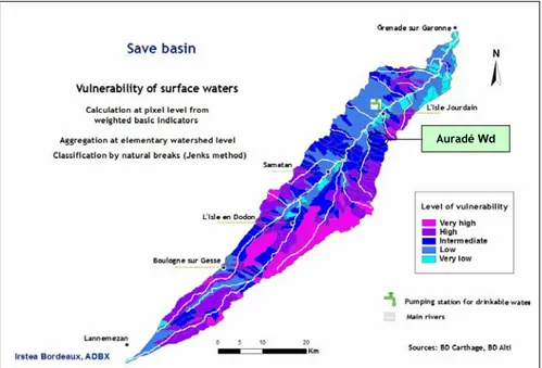
3.1. Vulnerability of surface waters in the Save watershed
Figure 5 shows the vulnerability of surface waters in the Save watershed based on three indicators: soil types, slopes, distance from watercourses. The vulnerability is higher in the Pyrenees piedmont because of higher slopes, narrow valleys, and superficial soils. We aggregated the values resulting from calculation of each pixel, to the elementary watershed level in order to show the differences in vulnerability on this larger watershed scale.
Figure 5. Surface water vulnerability, combining indicators of slopes, soils nature and hydrographic network with weighting obtained from MCDA model 3.2. Land use in 2009 in the Auradé watershed and the Save
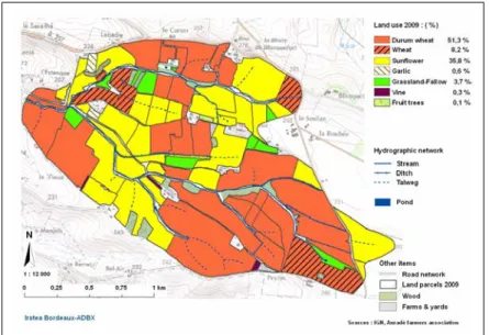
Figures 6 and 7 show respectively the land use in the Auradé watershed and the Save for the agricultural year 2009 and their very significant differences, even if the small Auradé area is part of the larger watershed.
The two maps show a major difference in the land use and agricultural practices on these two levels of watershed (Wd). In the Auradé Wd, the crop system is very intensive and the rotation is mostly binary: essentially wheat (60% of the area in
2009 and sunflower (36%). The wheat receives very doses of fertiliser (nitrogen, phosphorus, and potassium), whereas the sunflower crops receive little or no fertilisation in the second year of rotation (minimal use of nitrogen).
Figure 6. Land use in 2009 in the Auradé watershed
Figure 7. Land use in 2009, in save watershad
In the Save watershed, we can identify two main sections. Section 1 runs from the upstream area (south west) to the central zone, which mainly contains grassland and forest, with some cereal crops and corn. Section 2 extends from the central zone to the downstream area (north east). This second section has a considerable amount of intensive agriculture, with differing crop rotations: 2 to 3 years in the hills (as is the case with Auradé) and 3 to 4 years on the plains bordering the rivers. The crops in Section 2 include corn, soya bean, and sorghum.
3.3. Contamination risks from nitrogen transfers to watercourses
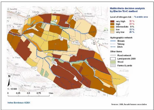
Figure 8 depicts results taking BEPs into account, calculated at the farming parcel level. It is important to note the 23% weighting given to BEP criteria in our model. Many other systems, such as physical models, do not consider this type of qualitative data at all.
A farming parcel must be in the same category of risk level, even if there are differences inside its area. This is a choice at decision-making level by farmers when applying the MCDA method. Despite this, the two categories of very high and high risks represent 55% of the Used Agricultural Area (UAA), 8% in the intermediate category and 38% in the low category.
Figure 8. Risks of nitrogen transfers in surface waters in 2009 in the Auradé watershed
These results were validated by nitrogen samples in the downstream of Auradé Wd, which showed very high concentrations in streams directly after these chemicals were applied. The highest content recorded was almost 150 mg/l. The average figure, based on samples taken over twenty years appears around 50 mg/L (Ferrant et al., 2011), (Table 5: measuring station P5). This considerably exceeds the values laid down in the Europan standards for the quality of drinking water. When the ineffectiveness of BEPs is incorporated into a simulation for 2009, 58% of the UAA is ranked “high” for nitrogen transfer risk.
When we modelled the same risks in 2010, “high” risk accounted for 38% of the UAA, because of the predominance of sunflowers (50%) and the resulting reduction in nitrogen inputs.
The MCDA modelling can help local actors and decision makers (environmental managers) by making them aware of these high concentrations of nitrogen. In this environmental context, with very high slopes, impermeable substratum and many connections to the stream, BEPs are not sufficient to lower the level of nitrogen contamination in streams. This means that agricultural practices have to be drastically modified. Studying a small watershed is an effective way of seeing the results of decision making in the actual areas where these decisions are made.
Figure 9 depicts the nitrogen transfer risks for the Save Wd. Risks were first calculated at the pixel scale, and then aggregated at different spatial scales. In this map, results were aggregated to elementary watershed level. This is a decision making scale for managers and not for farmers, because the level of precision is lower: for instance the elementary watershed (Montoussé Wd) including that of Auradé is assigned in one risk category (very high).
The “high” and “very high” risk levels are less present in the larger watershed (43% of the UAA) because part of this area has little or no exposure to nitrogen. We can therefore assume that the smaller the organisational level, the higher the resulting figures tend to be.
Forty-three percent of the Save watershed has a risk ranking of “high” and “very high”. These values are of course lower than the Auradé watershed, because many crops outside of the area receive little or no nitrogen. We can therefore assume that the smaller the organisational level, the higher the resulting figures tend to be. For information, 28.8% of farmland in the entire Save area falls into the “intermediate” risk category (as opposed to just 8% for Auradé).
Part of an area can change to a higher or lower risk category, depending on the agricultural pressure applied, i.e. land use and farming practices. If grasslands are replaced by crops such as wheat and rape seed, the risk level will increase, because a significant part of areas sorted into the intermediate risk are located in the upstream portion of the Save watershed (Figure 7).
On the other hand, if intensive crops (wheat, rape seed) are replaced by extensive crops (barley, sunflower), or if the fertilisation level is lower, the risk level can decrease.
From a more general point of view, it can be said that when conventional agricultural methods are replaced by an approach that considers the welfare of the environment, the likelihood is that surface water contamination risks will be reduced.
We can see the two parts of the Save Watershed, whose land use was described in 2009. Part 1 has lower nitrogen risks than part 2.
Another problem encountered during aggregation is where pixels are located on the edges of sub-basins. These pixels are included in the risk calculation of the neighbouring watershed, which can lead to inaccuracies.
Using an elementary watershed and hydrological area means that each spatial unit receives its own risk score. We have to accept that certain information will be lost, and using an average score can help to smooth out the risk values as determined at pixel level.
Figure 9. Risks of nitrogen transfers in the Save watershed surface waters, in 2009, using differentiated weights of vulnerability indicators
These results were obtained using differently weighted vulnerability indicators through the MCDA model. As a reminder, these were slopes (38%), soil types (15%), and connectivity (47%). These were compared with equal weights (table 4) at pixel level and then at the elementary watershed level after aggregation.
This gives us certain conclusions. Firstly, at pixel level, differentiated weights led to an increase in areas of “very high” and “high” risk (around 39%), and an greater level of risk for “intermediate” areas (29%). Low risk areas saw a drop (32%). There was an overall increase in “high” risk zones, representing 18.2% across the entire area. This can be explained by the fact that the upstream part of the Save watershed falls within the Pyrenean piedmont. In addition to this, there are higher slopes, and a denser hydrologic network. These two elements mean that the risk values in the pixel calculation are higher.
At elementary watershed level, we can see some minor differences resulting from the “smoothing” process. With vulnerability weighting, the area classified “very high” in terms of transfer risks decreases by 4.7%, and areas of “low” risk increase by the same proportion. At this scale, in the aggregated results, gaps are minor between a differentiated weighting of vulnerability indicators in comparison with equal weights. This is explained by the average values arrived at during aggregation. When dealing with managers, it is better to present average figures relevant to their decision-making area.
The Auradé watershed, studied using a MCDA method, appears as “very high” risk in the context of the Save watershed, which has been verified by field tests and with the results from the MCDA model.
The MCDA method parameters were useful in improving the parameters contained in the Azotopixal method.
In order to validate (or not) our results, we attempted to compare potential contamination risks by measuring nitrate concentration in watercourses. In order to do this, we had to first show contamination risks calculated at pixel level for the main watercourses. We also aggregated values upstream to downstream at the hydrological area level. By doing this, we were able to obtain mean values for river segments. Different teams took water samples from six measurement stations, starting upstream and then moving further downstream.
The Irstea Bordeaux Water Quality Lab team (formerly known as Cemagref) measured water quality between March and November 2008, in stations P1 to P4 (see Figure 10).
The ECOLAB team regularly sampled the quality of water at station P5, from July 2009 to June 2010. In P6, GPN-TOTAL (previously AZF Toulouse) took regular samples from the station on the Montoussé stream (Auradé watershed) from 1985 to 2004 (Ferrant et al., 2011);
Table 4. Comparison of MCDA differentiated-weight results, vulnerability indicators, and equally weighted results for nitrogen risks on the Save watershed
Table 5. Comparison between nitrogen contamination risk level in 2009, and average nitrate concentration in the six measurement stations Gauging
station
Nitrogen risk
level Average concentration of Nitrates (mg/L)
Highest concentration of Nitrates (mg/L) P1 Very low 7.3 12.7 P2 Very low 11.7 21.2 P3 Very low 13.1 24.0 P4 High 15.9 25.4 P5 High 23.7 66.0 P6 Very high 48.7 142.3
While the sample periods and methods were different, these results have been relatively constant in recent years, making them suitable for comparison with our own results (Figure 10 and Table 5).
Nitrogen transfer risks were assessed for farmland use in 2009. Our calculations did not take into account rainfall and evapotranspiration, as these parameters are not sufficiently discriminating for a multi-indicator spatial model. This was overcome by optimising AZOTOPIXAL with connectivity, thus providing a higher level of potential contamination in flood periods.
Samples were taken from the six different measurement stations during different periods. P1 to P5 were located directly on the Save River, and P6 was located on the
PIXEL level Elementary watershed level 2009
≠ weights weights Distance Equal ≠ weights weights Distance Equal
Classes % % % % % % Very high 16.3 5.2 11.1 11.4 16.1 -4.7 High 22.4 15.3 7.1 31.7 31.7 0 Intermediate 29.3 25.9 3.4 28.8 26.0 2.8 Low 24.1 30.9 -6.8 25.2 22.2 3.0 Very low 7.9 22.7 -14.8 2.9 4.0 -1.1 Total 100.0 100.0 – 100.0 100,0 –
small Montoussé stream, in the heart of the Auradé watershed, of intense farming activity. While we only obtained 8 samples in P1 to P4, continuous samples were taken in P5 and P6.
Table 5 depicts the average and the highest values of nitrate concentration for each sampling period, listed by sampling station.
Despite the difficulty of only having six measurement sampling stations for water samples, and 8 samples in P1 to P4, it is interesting to see the different values (Table 5), and to compare them with the contamination risks, estimated through the AZOTOPIXAL method.
With the continuous samples in P5 and P6, the results are naturally more accurate and representative of flow and nitrate concentrations in watercourses, because our method was optimised for flood periods.
Figure 10. Cumulated risk values in Save watercourse and measuring stations for surface water
Nitrate concentration falls within acceptable average values in P1 to P5, because of the dilution in the Save river water. On the contrary, these concentrations are higher in the Montoussé stream in the heart of Auradé watershed. The value in P6 is the maximum legal average, and can triple during periods of increased fertiliser use.
As with nitrate sampling, our method allowed us to provide a clear representation of the potential risk of nitrate concentration both upstream and downstream of the Save watershed. The trend shown by our model partially validates the choice of method in these circumstances.
4. Conclusion and perspectives
We implemented two different kinds of methods for assessing contaminant transfer risks: a multi-criteria modelling method (ELECTRE TRI-C) combined with a GIS (ArcGIS®) on a small watershed, and one of the PIXAL methods, combining spatialised indicators for larger spaces. For a small elementary watershed, it was necessary to obtain results directly from the area where farmers’ decisions were implemented, i.e. on the farmland itself. Our method allows quantitative and qualitative criteria, such as Best Environmental Practices (BEPs) to be used for risk assessment. Because of this, we still needed to visit the study site ourselves to carry out observations.
In 2009, we used the 3 km² experimental watershed in Auradé, southwest France for the study of nitrogen transfer risks. Our results highlighted that a large proportion of farmland in this area (55%) fell into the “high” and “very high” risk category, even where BEPs were in force. This assertion is supported by water samples taken in downstream areas, which showed levels often exceeding the legal level of 50 mg/l.
While the MCDA method gave very precise results, it cannot be used on a large area, in the same conditions, because extensive field observations are necessary. For large watersheds, including the 1,150 km² Save, we used a different method, called AZOTOPIXAL (for nitrogen). This approach combined remote sensing and GIS to provide agro-environmental risk assessment on a pixel scale (30m x 30m). The scores for each indicator were refined using criteria scores, drawn from multi-criteria modelling. The weighting of MCDA multi-criteria was extrapolated to the vulnerability factors in the AZOTOPIXAL method.
Risk values were aggregated at several spatial scales, such as elementary watershed and hydrological area. 43% of the surface area of the greater watershed was classified “high” and “very high” risk, less than that for the Auradé watershed alone. This is due to the presence of grassland and different crops on which little or no fertiliser is used. Another reason for this is that results from the small watershed were obtained at agricultural parcel level, whereas results from the large watershed were calculated at pixel level, and then aggregated at elementary watershed level. The results from the large watershed were destined for use in decision-making by environmental managers. Despite these differences, 43% remains a very high figure for an area of only 1,150 km².
In order to check the accuracy of our results, we calculated average risk values along the watercourse of the Save, as well as those applying to its tributaries from an
aggregation at the hydrologic area scale. We compared the values we obtained with values measured at six points along the river. The results followed the same progression both upstream and downstream.
The AZOTOPIXAL method is unable to take into account BEPs and other qualitative data. This is also the case with agro-hydrological models. Because of this, the combination of the AZOTOPIXAL method with MCDA modelling can be very effective. Scores and weights can be tested on a smaller watershed, before applying them to a wider surface area. Both of the methods we used are of great help to decision makers, managers, and local stakeholders.
For the future, it would be interesting to adapt the MCDA method for a larger scale than that of an elementary watershed. It would also be beneficial to improve the accuracy of the AZOTOPIXAL method. Developments such as these merit further investigation, and could be of great benefit to the field of spatialised multi-criteria decision-making.
Acknowledgements
We would like to thank the EU-Interreg SUDOE IV B for funding this study, as part of the “Aguaflash” project. Our thanks also go to the association of Auradé farmers and especially their technician Vincent Gobert, for his active cooperation in this project. We thank also the laboratory teams of the Irstea-REBX unit and INPT-Ecolab for field samples and chemical analysis; Daniel Uny, geomatician in the Irstea-ADBX unit, for supporting the development of geomatic applications, and James Emery, English teacher and translator, for his help in proofreading this paper.
Bibliography
Almeida-Dias J., Rui-Figueira J., Roy B. (2010). ELECTRE TRI-C: A multiple criteria sorting method based on characteristic reference actions. European Journal of Operational Research, vol. 204, p. 565-580.
Arnold J.G., Srinivasan R., Muttiah R.S., Williams J.R. (1998). Large area hydrologic modeling and assessment. Part I: Model Development.The Journal of the American water resources association,vol. 34, n° 1, p. 73-89.
Beaujouan V., Durand P., Ruiz L., Aurousseau P., Cotteret G. (2002). A hydrological model dedicated to topography-based simulation of nitrogen transfer and transformation: Rationale and application to the geomorphology-denitrification relationship. Hydrological Processes, vol. 16, p. 493-507.
Bioteau T., Bordenave P., Laurent F., Ruelland D. (2002). Évaluation des risques de pollution diffuse par l’azote d’origine agricole à l’échelle de bassins versants : intérêts d’une approche par modélisation avec SWAT. Ingéniéries-EAT, vol. 32, p. 3-12.
Blöschl G., Sivapalan M. (1995). Scale issues in hydrological modelling: a review, John Wiley & sons, Chichester, GBR.
Carluer N., Tournebize J., Gouy V., Margoum C., Vincent B., Gril J.J. (2009). Role of buffer zones in controlling pesticides fluxes to surface waters. Procedia Environmental Sciences. Chen Y., Khan S., Paydar Z. (2010). To retire or expand? A fuzzy GIS-based spatial multi-criteria evaluation framework for irrigated agriculture. Irrigation and Drainage, vol. 59, n° 2, 2010, p. 174-188.
CE (1991) Directive du Conseil n° 91/676/CEE du 12 décembre 1991, concernant la protection des eaux par les nitrates à partir de sources agricoles, JOCE, n° L 375, 31 décembre 1991.
CE (1998) Directive n° 98/83/CE du 03/11/98 relative à la qualité des eaux destinées à la consommation humaine, JOCE, 5 décembre 1998.
Chakhar S., Mousseau V. (2008). GIS-based multi-criteria spatial modelling generic framework. International Journal of Geographical Information Science, vol. 22, n° 11-12, p. 1159-1196.
CORPEN2006. Des indicateurs AZOTE pour gérer des actions de maîtrise des pollutions à l’échelle de la parcelle, de l’exploitation et du territoire, Paris, MAP-MEDD,
CORPEN2007. Produits phytosanitaires et dispositifs enherbés. Etat des connaissances et propositions de mise en oeuvre, Paris, MAP-MEDD.
EC, Directive 2000/60/EC of the European Parliament and of the Council of 23 October 2000 establishing a framework for Community action in the field of water policy. Official Journal of the European Communities, 2000.
FAO, Best Available Techniques (BAT) and Best Environmental Practice (BEP) Series, Paris Commission’s Working Group on Diffuse Sources (DIFFCHEM), Paris. 1997.
Fealy R.M., Buckley C., Mechan S., Melland A., Mellander P.E., Shortle G., Wall D., Jordan P. (2010). The Irish Agricultural Catchments Programme: catchment selection using spatial multi-criteria decision analysis. Soil use and management, vol. 26, n° 3, p. 225-236.
Ferrant S., Oehler F., Durand P., Ruiz L., Salmon-Monviola J., Justes E., Dugast P., Probst A., Probst J.-L., Sanchez-Perez J.-M. (2001). Understanding nitrogen transfer dynamics in a small agricultural catchment: Comparison of a distributed (TNT2) and a semi distributed (SWAT) modeling approaches. Journal of Hydrology, vol. 406, p. 1-15. Figueira J., Roy B. (2002). Determining the weights of criteria in the ELECTRE type methods
with a revised Simos procedure. European Journal of Operational Research, vol. 139, p. 317-326.
Gomez E., Ledoux E., Viennot P., Mignolet C., Benoit M., Bornerand C., Schott C., Mary B., Billen G., Ducharne A., Brunstein D. (2003). Un outil de modélisation intégrée du transfert des nitrates sur un système hydrologique : application au bassin de la Seine. La Houille Blanche, vol. 3, p. 38-45.
Gril J.J., Lacas J.G. (2004). Intérêt des zones tampons enherbées et boisées pour limiter le transfert diffus des produits phytosanitaires vers les milieux aquatiques. De l’état des connaissances aux recommandations pratiques, Cemagref, Lyon.
Hénin S. (1980). Rapport du groupe de travail activités agricoles et qualité des eaux. Synthèse, ministère de l’Agriculture et ministère de l’Environnement et du Cadre de vie. Kirchrnann H., Katterer T., Andrén O. (2005). Organic Farming - 1s this the Way Forward?
Some highlights from comparative studies. International Workshop where do fertilizers go?, G.B. Bouraoui Faycal, Mulligan D., Galbiati L., European commission – JRC - Institute for Environment and Sustainability Belgirate, p. 1-15.
Janssen R., Rietveld P. (1990). Multi-criteria analysis and GIS: an application to agricultural landuse in The Netherlands. Scholten and Stillwell (Eds.), Kluwer, Dordrecht.
Joerin F., Musy A. (2000). Land management with GIS and multi-criteria analysis. International transactions in Operational Research, vol. 7, p. 67-78.
Laaribi A. (2000). SIG et analyse multicritère. Hermès Sciences Publications, Paris,
Lafitte J.-J., Cravero G. (2010). La généralisation des bandes enherbées le long des cours d’eau (article 52 du projet de loi Grenelle 2) : réflexion sur l’impact et la mise en œuvre de cette disposition, Ministères français chargés de l’Environnement (MEDDAD) et de l’Agriculture (MAP), Paris,
Macary F., Lavie E., Lucas G., Riglos O. (2006). Méthode de changement d’échelle pour l’estimation du potentiel de contamination des eaux de surface par l’azote. Ingénieries-EAT, n° 46, p. 35-49.
Macary F., Vernier F. (2007). Zonage de risque potentiel de transferts de pesticides à l’échelle de bassins versants : quelles méthodes pour un transfert d’échelles spatiales ?, Pesticides : impacts environnementaux, gestion et traitements, Presses de l’École Nationale des Ponts et Chaussée, Paris.
Macary F., Leccia O., Uny D., Petit K. (2010a). Usage de la Géomatique afin de déterminer les zones à risque agro-environnemental pour la qualité des eaux de surface. Colloque francophone ESRI, Versailles, 29-30 septembre.
Macary F., Ombredane D., Uny D. (2010b). A multi-criteria spatial analysis of erosion risk into small watersheds in the low Normandy bocage (France) by ELECTRE III method coupled with a GIS. International Journal of Multi-criteria Decision Making, vol. 1, p. 25-48.
Macary F., Almeida-Dias J., Uny D., Probst A. Assessment of the effects of Best Environmental Practices on reducing pesticide pollution in surface water, using multi-criteria modelling combined with a GIS. International Journal of Multi-multi-criteria Decision Making, in Press, corrected proof.
Malczewski J. (2006). GIS-based multi-criteria decision analysis: a survey of the literature. International. Journal of Geographical Information Science, vol. 20, p. 703-726.
MATE, Décret n° 2001-34 du 10 janvier 2001 relatif aux programmes d’action à mettre en œuvre en vue de la protection des eaux contre la pollution par les nitrates d’origine agricole, JORF, 10 janvier 2001.
Maystre L.Y., Pictet J., Simos J. (1994). Méthodes multicritères ELECTRE. Description, conseils pratiques et cas d’application à la gestion environnementale, Paris, TEC & DOC, Lavoisier.
MEDDTL, Le Grenelle de l’Environnement. Synthèse, rapport du groupe n° 4 : adopter des modes de production et de consommation durables. ministère français de l’Écologie du Développement durable des Transports et du Logement, 2007.
MEDDTL, Le Grenelle de l’Environnement. Loi Grenelle II, Rapport, Paris, ministère français de l’Écologie et du Développement durable des Transports et du Logement, 2010. Mendas A., Delali A. (2010). Integration of MultiCriteria Decision Analysis in GIS to develop land suitability for agriculture: Application to durum wheat cultivation in the region of Mleta in Algeria. Computers and Electronics in Agriculture, vol. 83, p. 117-126. Misra A.K., Baker J.L., Mickelson S.K., Shang H. (1996). Contributing area and
concentration effects on herbicide removal by vegetative buffer strips. American Society of Agricultural and Biological Engineers, vol. 39, p. 2105-2111.
Mousseau V., Slowinski R., Zielnielwicz P. (2000). A user-oriented implementation of the ELECTRE-TRI method integrating preference elicitation support. Computers & Operations Research, vol. 27, p. 757-777.
OECD (2008). Environmental Performance of Agriculture in OECD Countries since 1990, OECD, Paris.
Oehler F., Durand P., Bordenave P., Saadi Z., Salmon-Monviola J. (2009). Modelling denitrification at the catchment scale. Science of The Total Environment, vol. 407, p. 1726-1737.
Oeurng C., Sauvage S., Sánchez-Pérez J.-M. (2011). Assessment of hydrology, sediment and particulate organic carbon yield in a large agricultural catchment using the SWAT model. Journal of Hydrology, vol. 401, p. 145-153.
Passuello A., Cadiach O., Perez Y., Schuhmacher M. (2012). A spatial multicriteria decision making tool to define the best agricultural areas for sewage sludge amendment. Environment International, vol. 38, n° 1, p. 1-9.
Perrin A.S., Probst A., Probst J.L. (2006). Impact of nitrogen fertilizers on natural weathering processes: Evident role on CO2 consumption., Geochimica & Cosmochimica Acta,
vol. 70, 483.
Probst J.L. (1985). Nitrogen and phosphorus exportation in the Garonne Basin (France). Journal of hydrology, vol. 76, p. 281-305.
Reshmidevi T., Eldho T., Jana R. (2010). Knowledge-Based Model for Supplementary Irrigation Assessment in Agricultural Watersheds. Journal of Irrigation and Drainage Engineering, vol. 136, n° 6, p. 376-382.
Roy B. (1968). Classement et choix en présence de points de vue multiples (la méthode Electre). Revue française d’informatique et de recherche opérationnelle, vol. 2, n° 8, p.57-75.
Roy B., Bouyssou D. (1993). Aide multicritère à la décision : méthodes et cas, Paris, Economica.
Sánchez-Pérez J.-M., Antiguedad I., Arrate I., García-Linares C., Morell I. (2003). The influence of nitrate leaching through unsaturated soil on groundwater pollution in an agricultural area of the Basque country: a case study. Science of The Total Environment, vol. 317, p. 173-187.
Schärlig A. (1985). Décider sur plusieurs critères, panorama de l’aide à la décision multicritère, Lausanne, Presses polytechniques et universitaires romandes.
Schärlig A. (1996). Pratiquer Electre et Prométhée. Un complément à Décider sur plusieurs critères, Lausanne, Presses polytechniques et universitaires romandes.
Schlosser I.J., Karr J.R. (1985). Riparian Vegetation and Channel Morphology Impact on Spatial Patterns of Water Quality in Agricultural Watersheds. Environmental Management, vol. 5, n° 3, p. 232-243.
Schmitt T.J., Dosskey M.G., Hoagland K.D. (1999). Filter Strip Performance and Processes for Different Vegetation, Widths, and Contaminants. Journal of Environmental Quality, vol. 28, p. 1479-1489.
Sebillotte M. (1992). Pratiques agricoles et fertilité du milieu. Économie rurale, n° 208-209, p. 117-124.
Simos J. (1990). Évaluer l’impact sur l’environnement. Une approche originale par l’analyse multicritère et la négociation, Lausanne, Presses polytechniques et universitaires Romandes.
Tiwari D.N., Loof R., Paudyal G.N. (1999). Environmental-economic decision-making in lowland irrigated agriculture using multi-criteria analysis techniques. Agricultural Systems, vol. 60, n° 2, p. 99-112.
Turpin N., Vernier F., Joncour F. (1997). Transfert des nutriments des sols vers les eaux - influence des pratiques agricoles. Ingénieries-EAT, vol. 11, p. 3-16.
Weyerbrock S. (1998). Reform of the European Union’s Common Agricultural Policy: How to reach GATT-compatibility? European Economic Review, vol. 42, p. 375-411.