Streamwise Fluidelastic Instability of Tube Arrays Subjected to Two-Phase Flow

(1)

UNIVERSITÉ DE MONTRÉAL

STREAMWISE FLUIDELASTIC INSTABILITY OF TUBE ARRAYS SUBJECTED TO TWO-PHASE FLOW

STEPHEN OKOTH OLALA

DÉPARTEMENT DE GÉNIE MÉCANIQUE ÉCOLE POLYTECHNIQUE DE MONTRÉAL

THÈSE PRÉSENTÉE EN VUE DE L’OBTENTION DU DIPLÔME DE PHILOSOPHIAE DOCTOR

(GÉNIE MÉCANIQUE) AOÛT 2016

(2)

ÉCOLE POLYTECHNIQUE DE MONTRÉAL

Cette thèse intitulée :

STREAMWISE FLUIDELASTIC INSTABILITY OF TUBE ARRAYS SUBJECTED TO TWO-PHASE FLOW

présentée par : OLALA Stephen Okoth

en vue de l’obtention du diplôme de : Philosophiae Doctor a été dûment acceptée par le jury d’examen constitué de :

M. REGGIO Marcelo, Ph. D., président

M. MUREITHI Njuki William, Ph. D., membre et directeur de recherche M. GOSSELIN Frédérick, Doctorat, membre

(3)

iii

ACKNOWLEDGEMENTS

First and foremost I would wish to thank my research supervisor, Prof. Njuki W. Mureithi, for his support, motivation and encouragement. Without his constant feedback and guidance, this Ph.D. would not have been achievable.

I would also like to express my gratitude to the staff at Polytechnique Montréal who offered various technical assistance. Mr. Noor Aimène for instrumentation of the strain gauges and Mr. Benedict Bésner for helping with the electronic devices installation and configuration; his immense knowledge on instrumentation and National Instrument data acquisition systems is commendable. Special mention goes to Mr. Thierry Lafrance, currently of Mekanic inc., for his guidance on technical design and modification of the test section.

I cannot forget the contribution of Teguewinde Sawadogo, currently at CNL, for sharing his experience on experimentation at the initial stages of the Ph.D. project.

I am grateful to the BWC/AECL/NSERC Industrial Chair of Fluid-Structure Interaction (FSI) for the financial support to pursue the Ph.D. program. Special recognition is due to the members of the FSI lab, especially Abdallah Hadji and Hao Li for their availability, encouragement and criticism, and Cedric Benguin for his help in the translation process of “Résumé”.

To all the friends who helped me remain focused during the Ph.D. program, I say a big thank you. Finally, I convey my deepest sense of gratitude and respect to my wife Florence and children, Imani, Adley and Marlone for their encouragement and unfailing love in spite of enduring my absence during the Ph.D journey.

(4)

RÉSUMÉ

Les vibrations induites par les écoulements est une préoccupation majeure pour les concepteurs et les opérateurs des échangeurs de chaleur. Parmi les nombreux mécanismes d'excitation, l'instabilité fluide-élastique a été identifiée comme la source la plus catastrophique de défaillance de tube à court terme dans les faisceaux. Par conséquent, un certain nombre de théories ont été mis au point pour sa prédiction. Cependant, toutes ces théories ont été développées principalement pour l'écoulement de monophasique, même si les faisceaux de tubes dans les générateurs de vapeur fonctionnent principalement en écoulement diphasique.

L'objectif principal de ce projet de recherche est donc d'étendre les modèles théoriques de l'instabilité élastique aux écoulements diphasique, en particulier, par l’instabilité fluide-élastique dans le sens de l’écoulement avec de multiples tubes flexibles. Le modèle quasi-statique a été étudié dans le cadre du projet de recherche en cours. L'étude a été réalisée pour un faisceau de tube triangulaire tourné.

Premièrement, des tests expérimentaux ont été réalisés afin de déterminer les forces quasi-statiques sur une grappe de tubes soumis à un écoulement diphasique transverse eau-air. Les tests ont été effectués pour une série de taux de vide et un nombre de Reynolds (en fonction de la vitesse inter tubé), 4

Re7.2 10 . Les forces obtenues et leurs dérivés spatiales en fonction de la position du tube central de la grappe ont ensuite été utilisées pour effectuer une analyse quasi-statique de l'instabilité fluides-élastiques. Les vitesses prévues d'instabilité ont été jugés en assez bon accord avec les tests de stabilité dynamique. La stabilité du faisceau de tubes a été trouvée en fonction du nombre et de l'emplacement des tubes flexibles. Entant donné que l'effet du déphasage a été ignoré à ce stade, l'analyse a confirmé la prédominance du mécanisme contrôlé par la rigidité pour provoquer une instabilité fluide-élastique dans le sens de l’écoulement. L'effet de désaccorder dans les fréquences naturelles des tubes sur le seuil d'instabilité a aussi été exploré. On a constaté que cet effet a en général un effet stabilisant. Cependant, pour un grand écart initial dans une population de fréquences, il a été constaté qu’un plus petit échantillon tiré de la population plus large puisse parfois avoir un écart inférieur ou supérieur résultant d’une grande dispersion des valeurs possibles de la constante de stabilité.

(5)

v Deuxièmement, les forces fluides instationnaires ont été mesurées sur la même grappe de tubes lorsque le tube central oscille dans la direction d'écoulement. Il a été trouvé que l’amplitude de la force de fluide instationnaire est une fonction dépendant uniquement de la vitesse réduite, et que pour des valeurs élevées de la vitesse réduite, elle est indépendante de la vitesse réduite. Les forces fluides induites sur les autres tubes ont cependant montré une dispersion importante probablement en raison de la faiblesse de la cohérence entre le mouvement du tube central et ces forces induites.

Les forces fluides instationnaires et les forces quasi-statiques obtenues dans la première série d'expériences ont ensuite été utilisées pour estimer, d'une part, le retard (déphasage) entre le mouvement du tube central et les forces de fluide sur lui-même et d'autre part, le retard entre le mouvement du tube central et les forces de fluide produites sur les tubes adjacents. Ce décalage temporel a été extrait pour chacun des tubes et le paramètre de retard et obtenu pour les taux de vide compris entre 60% et 90%. Ce paramètre de retard a montré une dépendance importante à la position du tube et au taux de vide.

Troisièmement, la masse ajoutée et l'amortissement indépendant de la vitesse de l’écoulement sur un tube contraint de vibrer seulement dans la direction de l'écoulement ont été déterminés expérimentalement. Il a été observé que la masse ajoutée diminue avec le taux de vide. L'amortissement d'autre part, augmente presque linéairement avec le taux de vide jusqu'à environ un taux de vide de 40%, puis reste relativement constant jusqu'à un taux de vide de 70%, puis enfin diminue à mesure que l’écoulement se rapproché d’un écoulement monophasique de gaz. Finalement, avec tous les paramètres nécessaires obtenus, le modèle quasi-statique a été utilisé pour prédire la vitesse critique d'instabilité fluide-élastique dans le sens de l’écoulement pour de multiples combinaisons de tubes flexibles au sein d’un réseau de tube triangulaire tourné soumis à un écoulement diphasique. L'utilisation du paramètre de retard déterminé expérimentalement n’affecte pas de manière significative la prédiction de la vitesse critique d'instabilité fluide-élastique pour les multiples configurations analysées. Les résultats obtenus avec le modèle quasi-statique, lorsque le paramètre de retard a été omis, étaient toujours en assez bon accord avec les données expérimentales.

(6)

La présente analyse a, en particulier, démontré le potentiel du modèle quasi-stationnaire pour la prédiction du seuil d'instabilité fluides-élastiques dans le sens de l’écoulement dans des faisceaux de tubes soumis à un écoulement transverse diphasique.

(7)

vii

ABSTRACT

Flow induced vibration is a major concern to designers and operators of tube-and-shell heat exchangers. Among the several excitation mechanisms, fluidelastic instability has been identified to be the most catastrophic source of tube failure in the short term in tube bundles. Consequently, a number of theories have been developed for its prediction. However, all these theories were developed primarily for single phase flow even though tube arrays in steam generators operate mostly in two-phase flow.

The main goal of this research project is therefore, to extend the theoretical models for fluidelastic instability to two-phase flow, particularly, streamwise fluidelastic instability of multiple flexible tube arrays in two-phase flow. The quasi-steady model has been studied in the scope of the current research project. The study was conducted for a rotated triangular array of pitch-to-diameter ratio ,P D 1.5.

Firstly, experimental tests were performed to determine the quasi-steady forces on a kernel of tubes subjected to two-phase air-water cross-flow. The tests were done for a series of void fractions and a Reynolds number (based on the pitch velocity), Re7.2 10 . 4 The forces obtained and their derivatives with respect to the static streamwise displacement of the central tube in the cluster were then used to perform a quasi-steady fluidelastic instability analysis. The predicted instability velocities were found to be in fairly good agreement with dynamic stability tests. Array stability was found to depend on the number and location of the flexible tubes. Since the effect of the time delay was ignored at this stage, the analysis confirmed the predominance of the stiffness-controlled mechanism in causing streamwise fluidelastic instability.

The effect of frequency detuning on the streamwise fluidelastic instability threshold was also explored. It was found that frequency detuning has, in general, a stabilizing effect. However, for a large initial variance in a population of frequencies, a smaller sample drawn from the larger population was found to sometimes have lower or higher variance resulting in a large scatter in possible values of the stability constant.

Secondly, the unsteady fluid forces on the same kernel of tubes were measured when the central tube was oscillated in the flow direction. The measured unsteady streamwise fluid force coefficient magnitude was found to be a single valued function of the reduced velocity, and

(8)

showed no dependence on the reduced velocity for high values of the reduced velocity. The cross-coupling fluid force phase, however, showed scatter possibly due to weak coherence between the central tube motion and the induced forces. The unsteady fluid forces together with quasi-steady forces obtained in the first set of experiments were then used to estimate, firstly, the time delay between the central tube motion and fluid forces on itself and secondly, the time delay between the central tube motion and the fluid forces generated on the adjacent tubes. The time lag/lead was extracted for each of the tubes and the time delay parameter obtained for void fractions between 60%-90% due to test loop limitations. The time delay showed significant dependence on tube position and void fraction.

Thirdly, the hydrodynamic mass and flow independent damping on a tube constrained to vibrate only in the streamwise direction in the array were experimentally determined. The hydrodynamic mass was observed to decrease with void fraction. The damping on the other hand, was found to increase almost linearly with void fraction till about 40% void fraction, remained fairly constant till 70% void fraction, then decreased as the flow approached single phase gas flow.

Finally, with all the necessary parameters obtained, the quasi-steady model was used to predict the critical velocity for streamwise fluidelastic instability of multiple flexible tubes in a rotated triangular tube array subjected to two-phase flow. The use of the experimentally determined time delays was found not to significantly affect the reduced critical velocity for streamwise fluidelastic instability of the multiple flexible tubes configurations analyzed. The results obtained with the quasi-steady model were in fairly good agreement with experimental data.

The present analysis has, in particular, demonstrated the potential of the quasi-steady model in predicting streamwise fluidelastic instability threshold in tube arrays subjected to two-phase cross-flow.

(9)

ix

LIST OF TABLES

Table 2-1 : Comparison of the physical properties of two-phase mixtures of air-water, steam-water, Freon R-11 and Freon R-22 (Feenstra et al., 1995; Feenstra et al., 2002) ... 17 Table 3-1 : Equivalent force coefficients derivatives ... 51 Table 3-2 : Total damping factor (structural + flow independent) for various void fractions (Olala

et al., 2014) ... 54 Table 4-1 : Time delay parameter ( ) dependence on void fraction and tube position for the

(14)

LIST OF FIGURES

Figure 2-1 : Vibratory response of a tube in a bundle as a function of flow speed (Blevins, 1990). ... 5 Figure 2-2 : Fluid coupling between adjacent tubes in an array ... 8 Figure 2-3 : Flow regime map proposed by Ulbrich & Mewes (1994). B-Bubbly, I-Intermittent

and D-Dispersed ... 14 Figure 2-4 : Flow regime maps proposed by Noghrehkar et al. (1999): Comparison with Ulbrich

& Mewes (1994) map in dotted lines. (a) In-line tube bundle (b) staggered tube bundle .... 14 Figure 2-5 : ASME fluidelastic instability design guideline map for heat exchangers (Weaver,

D.S. & Fitzpatrick, J. A., 1988) ... 19 Figure 2-6 : Idealized model of jet-flow between two cylinders in a staggered row of cylinders

(Roberts, 1962) ... 20 Figure 2-7 : Comparison between theoretical and experimental fluidelastic instability boundaries;

○, multiple flexible tubes in liquid flow; ●, multiple flexible tubes in gas flow; □, single flexible tube in gas flow; (─), Roberts(1966); (---), Connors (1970); (…), Blevins (1974). Adapted from (Price, 1995) ... 21 Figure 2-8 : Idealized cylinder motion of neighboring cylinders used by Connors (1970) during

force measurements on the central cylinder: (a) symmetric motion (b) antisymmetric motion (Païdoussis et al., 2011) ... 23 Figure 2-9 : Representation of cylinder numbering system used by Tanaka & Takahara (1980). 23 Figure 2-10 : Typical flow pattern through a staggered tube array ... 25 Figure 2-11 : Theoretical stability boundaries for fluidelastic instability obtained by Lever &

Weaver (1986b) for a single flexible tube in a parallel triangular tube array P 1.375;

 

 , practical stability boundary,



   , theoretical stability boundary. ... 27



Figure 2-12 : Fluid forces on a typical tube in a tube bundle... 29 Figure 3-1 : Two-phase test loop and array configuration ... 44

(15)

xv Figure 3-2 : Test section ... 44 Figure 3-3 : Instrumented tubes (a) central tube mounted on linear motor and (b) instrumented

neighboring tube ... 45 Figure 3-4 : Variation of tube C drag and lift coefficients with streamwise dimensionless

displacement of tube C ... 48 Figure 3-5 : Variation of tube 1 drag and lift coefficients with streamwise dimensionless

displacement of tube C ... 50 Figure 3-9 : Variation of the derivative of the drag coefficients with void fraction for (a) tubes C,

2 and 4 (b) tubes 1 and 3 ... 52 Figure 3-10 : Flexible tubes configuration for stability analysis - single column... 56 Figure 3-11 : Flexible tubes configuration for stability analysis - multiple columns ... 56 Figure 3-12 : Effect of the number of flexible tubes on the critical velocity for a column of tubes

(Refer to Figure 3-10) ... 57 Figure 3-13 : Effect of the number of flexible tubes on the critical velocity for multiple columns

of tubes (Refer to Figure 3-11) ... 57 Figure 3-14 : Comparison between present analysis and dynamic stability test (a) Flexible central

cluster (Figure 3-11(f)) (b) Two-partially flexible columns (Figure 3-11(d)) ... 59 Figure 3-15 : Instability map: comparison of present analysis with published data, ▼ two flexible

columns in air-water two-phase flow with tubes flexible in flow (present analysis), two partially flexible columns in air-water two-phase flow (present analysis), flexible central cluster in air-water two-phase flow (present analysis), a fully flexible array in air-water

(16)

two-phase flow (present analysis), axisymetrically flexible tube bundles in air-water two-phase flow (Pettigrew, Tromp, et al., 1989), ■ a single flexible column in air flow with tubes flexible in flow (Mureithi et al., 2005), ► a central flexible cluster in air flow with tubes flexible in flow (Mureithi et al., 2005), □ a central flexible cluster in air-water two-phase flow with tubes flexible in flow, f _n 28 Hz (Violette et al., 2006), a central flexible cluster in air-water two-phase flow with tubes flexible in flow, f n 14 Hz (Violette et al., 2006), ▲ two partially flexible columns in air-water two-phase flow with tubes flexible in flow (Violette et al., 2006). ... 61 Figure 3-16 : Evolution of eigenvalue with flow velocity for 90% void fraction, σ2=0 (0%

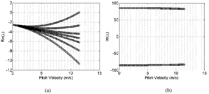
detuning) (a) real part (b) imaginary part ... 62 Figure 3-17 : Modes of Vibration for 90% void fraction, σ2=0 (0% detuning) (a) Unstable mode

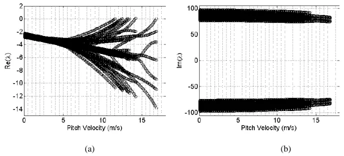
(mode 1) and (b) Mode 2 ... 63 Figure 3-18 : Evolution of eigenvalue for seven arrays, original population σ2=0.49 (5%

detuning) (a) real part and (b) imaginary part ... 64 Figure 3-19 : Evolution of eigenvalue for seven arrays, original population σ2=1.96 (10%

detuning): (a) real part and (b) imaginary part ... 64 Figure 3-20 : Evolution of eigenvalue for seven arrays, original population σ2=7.84 (20%

detuning) (a) real part and (b) imaginary part ... 65 Figure 3-21 : Effect of frequency detuning on streamwise stability constant (a) σ2=0.49 (5%

detuning) and (b) σ2_{=7.84 (20% detuning) ... 66} Figure 3-22 : Effect of random frequency detuning on streamwise stability constant,

2Hz f 14Hz ... 68 Figure 4-1 : Two-phase flow test loop and array configuration ... 75 Figure 4-2 : Test section for unsteady fluid forces cross-coupling measurements ... 75 Figure 4-3 : Instrumented tubes (a) central tube mounted on linear motor (b) instrumented

(17)

xvii Figure 4-4 : Variation of the unsteady streamwise fluid force coefficient with U fD for tube C,

0%

  ... 79 Figure 4-5 : Variation of the unsteady streamwise fluid force coefficient with U fD for  0%

(a-b) Tube 1, (c-d) Tube 4 ... 80 Figure 4-6 : Variation of the unsteady streamwise fluid force coefficient with U fD for  0%

(a-b) Tube 2, (c-d) Tube 3 ... 81 Figure 4-7 : Variation of the unsteady streamwise fluid force coefficient with U fD for tube C,

60%

  ... 83 Figure 4-8 : Variation of the unsteady streamwise fluid force coefficient with U fD for tube C,

80%

  ... 83 Figure 4-9 : Variation of the unsteady streamwise fluid force coefficient with U fD for

60%

  (a-b) Tube 1, (c-d) Tube 4 ... 84 Figure 4-10 : Variation of the unsteady streamwise fluid force coefficient with U fD for

60%

80%

  (a-b) Tube 2, (c-d) Tube 3 ... 87 Figure 4-13 : Effect of void fraction on the unsteady streamwise fluid force for 8 Hz Excitation

(Central tube, C) ... 89 Figure 4-14 : Effect of void fraction on the unsteady streamwise fluid force for 11 Hz Excitation

(Central tube, C) ... 89 Figure 4-15 : Effect of void fraction on the unsteady streamwise fluid force for 14 Hz Excitation

(18)

Figure 4-16 : Unsteady Fluid Force Phase Variation with _{U fD for tube C: (a)} 60% (b) 30  46 ... 93 Figure 4-17 : Unsteady Fluid Force Phase Variation with U fD for tube C: (a)  90% (b)

55  75 ... 93 Figure 4-18 : Time delay due to flow retardation for Tube C: (a, c) 60% void fraction (b, d) 80%

Void fraction;2.0 for 60% void fraction and 1.1 for 80% void fraction ... 97 Figure 4-19 : Time delays due to displacement of tube C for 60%VF (a, c) Tube 1 (b, d) Tube 4;

2.0

 for tube 1, 1.2 for tube 4... 100 Figure 4-20 : Time delays due to displacement of tube C for 60%VF (a, c) Tube 2 (b, d) Tube 3;

1.3

 for tube 2, 1.5 for tube 3 ... 101 Figure 4-21 : Time delays due to displacement of tube C for 80%VF (a, c) Tube 1 (b, d) Tube 4;

1.3

 for tube 1, 1.0 for tube 4 ... 102 Figure 4-22 : Time delays due to displacement of tube C for 80%VF: (a, c) Tube 2 (b, d) Tube 3;

2.2

 for tube 2, 1.3 for tube 3... 103 Figure 5-1 : (a) Test section (b) Flexible tube assembly ... 109 Figure 5-2 : Variation of the hydrodynamic mass ratio, m with void fraction: (a) Drag _R

comparison (b) comparison between drag and lift directions ... 111 Figure 5-3 : Variation of fluid flow independent damping with void fraction in streamwise and

transverse directions ... 111 Figure 5-4 : Flexible tubes configuration for stability analysis (a) single column, (b) two-partial

columns, (c) Central cluster ... 117 Figure 5-5 : Effect of the time delay on the reduced critical velocity for a flexible column of tubes

(Refer to Figure 5-4(a)) ... 118 Figure 5-6 : Effect of the time delay on the reduced critical velocity for two partially flexible

(19)

xix Figure 5-7 : Effect of the time delay on the reduced critical velocity for a kernel of flexible tubes (Refer to Figure 5-4(c)) ... 119 Figure 5-8 : Comparison between theoretical results (_r  _i  _exp) and experimental data

(Violette et al., 2006) for two partially flexible columns of tubes (Refer to Figure 5-4(b)) 120 Figure 5-9 : Comparison between theoretical results and experimental data (Violette et al., 2006)

for two partially flexible columns of tubes (Refer to Figure 5-4(b)) (a) _r _i  (b) 1 0

r i

   ... 121 Figure 5-10 : Comparison between theoretical results (_r  _i  _exp) and experimental data

(Violette et al., 2006) a kernel of flexible of tubes (Refer to Figure 5-4(c)) ... 122 Figure 5-11 : Comparison between theoretical results and experimental data (Violette et al., 2006)

for a kernel of flexible tubes (Refer to Figure 5-4(c)): (a) r i  and (b) 1 r i 0

(20)

LIST OF SYMBOLS AND ABBREVIATIONS

A Cross sectional area (m2)

 

C Damping matrix ,

D

C C L Drag coefficient, Lift coefficient

sh

C Dimensionless stiffness coefficient

F

C Unsteady fluid force coefficient

dh

C Dimensionless damping coefficient

D Tube diameter (m)

E Modulus of elasticity ( 2

/ N m ) FEI Fluidelastic instability

B

F Buoyancy force (N) ,

D

F F _L Corrected drag, lift force (N) ,

DM

F F_LM Measured drag, lift force (N)

LS

F Measured lift force in stationary liquid (N)

measured

F Measured fluid force per unit length

Uns

F Unsteady fluid force per unit length

F_{Uns cc}_{_} Cross-coupling unsteady fluid force per unit length

x

F Streamwise quasi-steady force per unit length

g Gravitational acceleration (m/s2), frequency dependent time delay parameter

I Moment of inertia ( 4 m )

 

I Identity matrix j   1

 

K Stiffness matrix K Connors constant

(21)

xxi L Tube length, distance between rows (m)

s

l Unsupported span length (m )

 

M Mass matrix

s

m Mass of tube per unit length

h

m Hydrodynamic mass per unit length

P Pitch between tubes (m)

,

g l

Q Q Gas, liquid volumetric flow rate (m3/s)

S Distance between tubes (m), velocity slip ratio SG Steam generator U_ Free-stream velocity (m/s) , p U U Pitch velocity (m/s) , eq c

U U Equivalent pitch velocity, critical velocity (m/s) ,

r

U Relative velocity (m/s)

,

x y Tube position in drag and lift direction (m)

q Generalized coordinates vector

x Dimensionless displacement with respect to D

 

x Dimensionless displacement vector

x Eigenvector

n

f Tube natural frequency (Hz)

,

m m a Structural, hydrodynamic mass per unit length (kg/m)

t Time (s)

, ,

h g l

   Two-phase, gas and liquid density (kg/m3₎ ,

  Void fraction

 Standard deviation

(22)

 Dynamic viscosity, time delay parameter

F

 Phase angle

 Dimensionless displacement, drag direction  Dimensionless displacement, lift direction

 Dimensionless time, time delay  Damping ratio

 Eigenvalue, dimensionless frequency factor , _n, _d

(23)

1

CHAPTER 1 INTRODUCTION

In a nuclear power plant, steam generators are used to convert liquid water to steam for purposes of driving turbines to produce electricity. Each of the steam generators contains thousands of tubes to maximize heat transfer. The “U” bend region of a recirculating-type nuclear steam generator experiences two-phase cross-flow that may induce structural vibrations and instability. Excessive vibrations could cause tube failure due to fatigue and fretting wear at the supports. These failures ordinarily lead to unscheduled plant shutdown and possible leakage of radioactive materials resulting in accidents and economic loss. Three mechanisms have been identified to be responsible for flow-induced vibrations in these components (Pettigrew & Taylor, 1991): turbulent buffeting which results from the unsteady forces developed on a tube due to exposure to the random pressure perturbations in the flow field, vortex shedding (flow periodicity) that leads to vibrations due to vortices shed when a fluid flows over a bluff body, and fluidelastic instability which is a self-excited mechanism in which vibrations result from the competition between energy input by the fluid and energy expended by the tubes. Of these vibration mechanisms, fluidelastic instability is the most dominant cause of tube failure in the short term, hence a major design consideration. As the flow velocity is increased, large tube vibrations occur. The larger the amplitude of the oscillation, the larger the resulting fluid dynamic force, leading to a rapid rise in oscillation amplitude with velocity. The velocity at which the fluidelastic forces balance the damping forces, characterized by a sharp increase in vibration amplitude, defines the threshold of fluidelastic instability and is referred to as the critical velocity. It is this critical velocity that is of importance to designing against fluidelastic instability.

Several theoretical models have been developed to deepen the understanding of fluidelastic instability phenomenon and estimate the critical velocity. These include the jet-switch model (Roberts, 1962), the quasi-static model (Blevins, 1974; Connors, 1970), the quasi-steady model (Price & Paidoussis, 1982, 1983), the unsteady model (Chen, 1983a, 1983b; Tanaka & Takahara, 1980), the semi-analytical model (Lever & Weaver, 1982, 1986a), the quasi-unsteady model (Granger & Paidoussis, 1996) and numerical models (Marn & Catton, 1990, 1991). Since these models were developed for single phase flow whereas most heat exchangers operate in two-phase flow, there is a need to extend and validate them in two-phase flow. All these models are carefully reviewed in this study.

(24)

Most of the reported flow-induced vibration experimental studies in two-phase flow have been done using air-water mixtures due to the high cost of operating steam-water loops. This raises the question of the validity of experimental results for tubes in a steam generator that, in practical situations, operate in steam-water mixtures. To overcome this problem, some researchers have used Freon due to the close proximity of its liquid/vapor density ratio to that of water/steam (Pettigrew & Taylor, 2009). However, Sawadogo (2016) recently demonstrated that there is no significant difference in the critical velocities obtained with both Freon and air-water mixtures. Air-water mixture is used in the present study.

Among the aforementioned fluidelastic instability models, the quasi-steady model (Price & Paidoussis, 1982, 1983) was chosen for the current study. This is due to the model’s ability to overcome the challenges posed by the other models, namely: the complexity of the two-phase flow making the implementation of the semi-analytical model (Lever & Weaver, 1982, 1986a, 1986b) cumbersome; enhanced experimental effort required by the unsteady model (Chen, 1983b; Tanaka & Takahara, 1980), the apparent multi-valued functional relation between the unsteady fluid force coefficient and the reduced velocity (Inada et al., 2002; Mureithi et al., 2002) and weak correlation between the tube displacement and the resulting unsteady fluidelastic forces (Mureithi et al., 2002) in two-phase flow. The computational fluid dynamic capabilities, at present, still rely on the other theoretical models and are confined to low Reynolds numbers. Studies conducted at the Fluid-Structure Interactions laboratory at École Polytechnique de Montréal by Shahriary et al. (2007) and Sawadogo & Mureithi (2014a, 2014b) successfully employed the quasi-steady model to investigate fluidelastic instability of tube bundles subjected to two-phase cross-flow. This model not only allowed the prediction of the critical velocity for instability but also the vibrational response of the cylinder as a result of fluid excitation.

The most important input parameters for the quasi-steady model are the quasi-steady forces and the time delay between tube displacement and the fluid forces generated thereby. Presently, the model has only been verified for vibration of a single flexible tube within a rotated triangular tube array in the transverse direction to the flow.

Until recently, most of the analysis on fluidelastic instability had been conducted for the direction transverse to the flow, after initial studies showed that fluidelastic instability occurred predominantly in that direction. However, recent tube failures at San Onofre Nuclear Generating

(25)

3 Station (SONGS) in U.S.A. (S.C.E., 2013) confirmed the possibility of fluidelastic instability occurring in the streamwise direction.

1.1 Objectives

The main goal of this Ph.D research project is to extend the existing knowledge on fluidelastic instability phenomenon in two-phase flows and validate the quasi-steady model for streamwise fluidelastic instability analysis. This is achieved by obtaining the necessary fluid force data through experimentation and employing the quasi-steady model to predict the critical velocity for streamwise fluidelastic instability of tubes in a rotated triangular array of P D 1.5.

To realize the global objective the project is divided into three phases. In the first phase, the flow direction quasi-steady fluid forces are experimentally determined for a central cluster of tubes in a rotated triangular array subjected to air-water two-phase flow. The derivatives of these forces are also obtained relative to the displacement of the central tube and, as a first approximation, the time delay is ignored. A stability analysis is then performed in the framework of the quasi-steady model to study the influence of the cross-coupling forces on the streamwise fluidelastic instability of the tube array under investigation. The effect of frequency detuning is also investigated in this phase. The quasi-steady fluid forces from this phase are passed on to the second phase to be used in the estimation of the time delay.

In phase two, the unsteady fluid forces on the kernel of tubes are measured to obtain the fluid force phases necessary for the estimation of the time delay. This is done for various excitation frequencies and void fractions. A wide range of flow velocities and frequencies are necessary to satisfy the assumption of the quasi-steady model whose input parameters are to be obtained. The method adopted for the extraction of the time delay requires the unsteady fluid forces and the corresponding quasi-steady fluid forces including their derivatives. The time delay parameters obtained in this phase are passed on to phase three.

Phase three is the analysis stage. Additional experiments are conducted to determine the flow independent damping and the hydrodynamic mass which are additional fluid-structure system characteristics. The parameters obtained in the previous phases are used to perform fluidelastic instability analysis for different configurations of the flexible tubes in the array. The results are then compared with dynamic test results in the literature to validate the model in two-phase flow.

(26)

1.2 Outline of the Thesis

The thesis begins with an introduction which includes the project objectives, methodology and the thesis outline. A detailed literature review follows in Chapter 2, focusing on flow induced vibration excitation mechanisms, theoretical models for fluidelastic instability and two-phase flow models.

The results are presented in the form of journal articles (Chapter 3-5). The first paper presented in Chapter 3 mainly focusses on the quasi-steady fluid forces. The second paper (Chapter 4) introduces the unsteady fluid forces and the time delay while the third paper (Chapter 5) presents the complete fluidelastic instability analysis using all the input parameters obtained in the previous papers/chapters. Model validation is also done in this chapter by comparing the model results with dynamic experiments’ data.

Finally, a general discussion of the results is made in Chapter 6 and recommendations for future work introduced in the Conclusion.

(27)

5

CHAPTER 2 LITERATURE REVIEW

2.1 Flow induced excitation mechanisms

Vibrations induced by fluid flow can be classified into three broad categories (Naudascher & Rockwell, 2005) namely forced vibrations, self-controlled vibrations and self-excited vibrations. Four excitation mechanisms have been identified for tube bundles subjected to cross–flow (Gorman, 1976; Pettigrew et al., 1991; Weaver, 1993): turbulent buffeting which is a forced vibration mechanism, vorticity shedding (Strouhal periodicity), and acoustic resonance which are self-controlled mechanisms, and fluidelastic instability, a self-excited mechanism. Figure 2-1 represents a typical vibratory response of a tube in a bundle subjected to cross-flow as a function of flow velocity (Blevins, 1990).

Figure 2-1 : Vibratory response of a tube in a bundle as a function of flow speed (Blevins, 1990).

2.1.1 Turbulent buffeting

Turbulent excitations result from the unsteady forces developed on a tube due to exposure to the random pressure perturbations in the flow field. Random velocity fluctuations from turbulent eddies spread over a wide range of frequencies producing random displacements of the tubes (Kuppan, 2000). While turbulent buffeting in steam generators is beneficial for heat transfer, the small vibration amplitudes caused by turbulence forces have to be estimated to determine the effective life of the equipment (Hassan et al., 2003). Turbulent buffeting in tube bundles is present at all flow velocities, but is only dominant before the critical velocity for fluidelastic

(28)

instability and vortex lock-in is reached. A detailed review of turbulent buffeting modeling techniques is introduced in Weaver et al. (2000)

2.1.2 Vortex shedding and general flow periodicities

Tube bundles subjected to cross-flow are generally excited by periodic fluid forces whose frequency vary linearly with flow velocity (Ziada & Oengoren, 1993). This phenomenon of periodic excitation is variously referred to in the literature as vortex shedding, periodic wake shedding or Strouhal excitation. There are many parameters that can affect the periodicity of vortex shedding. These include cylinder arrangement, cylinder pitch, upstream turbulence, vibration amplitude, surface roughness, two-dimensionality of the flow and the scale aspect ratio (Paidoussis, 1982). Vortex shedding on a single tube is markedly different from that in tube arrays where periodic forces have been noted in the upstream rows in single phase fluid flow. This periodicity is suppressed by turbulence deeper in the tube array (Weaver, 1993). Different array configurations experience different forms of periodicities. For instance, in staggered arrays, flow periodicity is caused by alternate vortex shedding from upstream rows whereas jet instability is the source of periodicity in normal square arrays (Weaver, 1993; Ziada & Oengoren, 1993). Ziada & Oengoren (1992) found that the flow structure, hence vortex shedding only occur in upstream rows for arrays with pitch-to-diameter,



P D ratio less than 1.5 while it persists



, over the entire array for those with P D 1.75 in an in-line tube bundle configuration.

Vortex shedding causes fluctuations in the drag forces at a frequency twice that of the lift (Weaver et al., 2000) and is scaled using a non-dimensional frequency parameter, Strouhal number, S : _t v t f D S U  (2-1)

where f is the frequency of vortex shedding, D is the diameter of the cylinder and U the fluid _v freestream velocity (Bearman, 1984). It is evident from Eq. (2-1) that the value of S depends on t

the flow characteristics. For sub-critical flow



40Re 2 105



, S _t 0.2, while S _t 0.3 for supercritical flow regime



Re3.5 10 6



for circular cylinders. The transition between these two

(29)

7 regimes is not well defined (Paidoussis, 1982). Detailed discussion of vortex shedding in tube bundles may be found in Weaver et al. (1987) and Ziada (2006).

In a situation where the vibration amplitude is greater than 0.01D and the mass-damping parameter, m ₂

D



 is not too large, vortex shedding frequency may coincide with the cylinder

natural frequency resulting in high amplitude oscillations, a phenomenon referred to as “lock-in”. To avoid resonance and lock-in due to vortex shedding the natural frequency should be kept

40%

 beyond f (Paidoussis, 1982). Alternatively, one may reduce the vibration amplitude by _v increasing the structural damping.

2.1.3 Fluidelastic instability

The third excitation mechanism in tube bundles is the fluidelastic instability. This phenomenon can be described as a self-excited feedback mechanism between tube motion and fluid forces. If the feedback is positive, meaning that the fluid force has a component in the positive velocity direction, net damping will decrease as the fluid flow velocity increases. At a certain flow velocity, commonly referred to as critical velocity

 

U_c , the net damping of the system vanishes, leading to high amplitude tube displacements potentially causing catastrophic failure. The spectrum of the response is characterized by a narrow peak revealing the absence of significant damping (Pettigrew & Taylor, 1991). To further illustrate what happens when the free stream flow reaches the critical velocity, consider a tube array subjected to cross flow as shown in Figure 2-2. The general equation of motion of the system may be expressed as:

 

Ms

 

x + C

 

s

 

x + K

 

s

   

x = Fext (2-2)

in which,

 

Ms is the structural mass matrix,

 

C is the structural damping matrix, s

 

Ks is the

structural stiffness matrix,

 

x is the tube acceleration vector,

 

x is the tube velocity vector,

 

x is the tube displacement vector and

 

F_ext is the fluid force vector for tube array subjected to cross flow.

 

Fext includes fluid added mass, fluid damping forces, and fluid stiffness forces

(30)

Figure 2-2 : Fluid coupling between adjacent tubes in an array The system’s equation of motion can therefore be written as:

   



M + Ms f



 

x + C + C



   

s f



 

x + K + K



   

s f



   

x = 0 (2-3)

where

 

M is the fluid added mass, _f

 

C is the fluid damping and _f

 

K is the fluid stiffness. _f The system is considered to be stable if the response motion diminishes with time, while it will be unstable if energy is fed into it through self-excitation with the response motion increasing with time (Rao, 2004). In order to guarantee system stability, both total damping and total stiffness terms in Eq. (2-3) should be positive.

Instability can be classified as either static or dynamic (Price, 1995). Static instability also known as divergence occurs when the negative fluid stiffness exceeds the structural stiffness leading to a negative total stiffness. As the total stiffness goes to zero the system’s natural frequency,  , _n shown in Eq. (2-4), also tends to zero. Static instability is therefore characterized by a frequency of oscillation approaching zero at stability threshold. Static instability is rarely experienced in heat exchanger tube arrays as dynamic instability normally occurs before it.

n

K M

(31)

9 Dynamic instability on the other hand can be caused by two main mechanisms (Chen, 1983a, 1983b; Paidoussis & Price, 1988): damping controlled and stiffness controlled mechanisms. Damping-controlled mechanism is predominant for low mass-damping parameter,



m D2



or high fluid density flows. This kind of instability occurs when the fluid force component in phase with the cylinder velocity overcomes the mechanical damping force leading to a negative total damping in the system. It only requires one-degree-of-freedom in which the destabilizing fluid force provides a negative damping effect. Stiffness-controlled instability which is predominant for low fluid density flows (high m D2), on the other hand, requires at least two-degrees-of-freedom (multiple-flexible tubes) such that the relative motion between tubes results in a net force that overcomes the structural damping.

2.1.4 Streamwise fluidelastic instability

A number of experimental studies (e.g. (Granger et al., 1993; Janzen et al., 2005; Mureithi et al., 2005; Nakamura et al., 2014; Roberts, 1962, 1966; Violette et al., 2006)) have reported observations of streamwise fluidelastic instability in both single- and two-phase flows. Roberts (1962), for instance, showed that instability was primarily in the streamwise direction (at least for tube rows) in liquid flow. Janzen et al. (2005) reported experimental evidence of streamwise two-phase flow induced fluidelastic instability in a rotated triangular U-tube array of pitch-to-diameter ratio, P/D=1.5. They observed streamwise fluidelastic instability in water flow and low-void fraction



25%



air-water two-phase flow. Mureithi et al. (2005) reported in-plane fluidelastic instability for a rotated triangular array with tubes preferentially flexible in the flow direction subjected to air flow. Their array

P D 

1.37

. Mureithi et al. (2005) determined streamwise fluidelastic instability for the case of fully flexible array and for a single flexible column in a rigid array. They, however, did not observe instability for a single flexible tube in a rigid array. Later, Violette et al. (2006) did a comprehensive experimental study of in-plane fluidelastic instability of a rotated triangular tube bundle of P/D=1.5 subjected to two-phase flow. They reported occurrence of fluidelastic instability for multiple tubes and not for a single tube only flexible in the flow direction. Recently, Nakamura et al. (2014) found that fluidelastic instability in the flow direction could occur at a lower critical flow velocity than that for the transverse flow direction in a fully flexible normal triangular array of small P/D (=1.2) subjected

(32)

to air flow. What is common in the above studies is the fact that streamwise fluidelastic instability was observed for multiple flexible tubes and not for a single flexible tube in a rigid array. This, therefore, suggests that streamwise fluidelastic instability is largely fluid stiffness controlled, requiring fluid coupling of different tubes in the array.

Details of the theoretical models for predicting fluidelastic instability in tube arrays subjected to cross-flow are discussed in section 2.3.

2.2 Two-phase flow induced vibrations

Even though numerous industrial components operate in two-phase flows, studies on vibration induced by this type of flow have grown only recently. The main excitation mechanisms in two-phase flows are turbulence and fluidelastic forces. Generally, forces due to the vortex shedding are absent for void fractions in excess of 15% (Taylor et al., 1989). The intensity and nature of the excitations induced by two-phase flows depend on several two-phase parameters which include void fraction, mass flow rate and flow regimes.

2.2.1 Two-phase flow models

The most important parameters in the study of vibrations induced by two-phase flows are void fraction, flow velocity and flow regime. Since measuring these parameters are complicated, several models have been developed for their estimation.

2.2.1.1 Homogeneous model

The homogeneous model assumes a uniform flow through the cross section of the channel with the gas and liquid phases traveling at the same velocity. In this model, the void fraction is equal to the volumetric flow fraction and is given by:

g l g Q Q Q    (2-5)

where Q is the volumetric flow rate, and the subscripts, g and, l denote the gaseous and liquid phases, respectively. The average homogeneous mass density and flow velocity of the two phase mixture are, respectively, expressed as:

(33)

11



1



h g l      (2-6) and g g l l h Q Q U A       (2-7)

where A is the cross-sectional area of the flow channel,  is the mass density and the subscript, h indicates homogeneous quantity. The pitch velocity,U_p, for tube bundles in cross-flow is defined as: p P U U P D    (2-8)

where U_ is the homogeneous velocity upstream of the tube bundles, P the pitch spacing between tubes and D the tube diameter.

The homogeneous model is widely used by researchers due to its simplicity, but under certain flow conditions, such as the case of vertical flow against gravity, the slip between the phases cannot be neglected. The homogeneous model gives best agreements in bubbly and dispersed or mist flow regimes where the entrained phase travels at nearly the same velocity as the uniform phase. The model is also the limiting case as the pressure tends towards the critical pressure, where the difference in phase densities disappears. Its use is also valid at very large mass velocities and at high vapor qualities (Thome, 2010).

2.2.1.2 Feenstra model

In the Feenstra et al. (2000) model, void fraction is presented as a function of the velocity ratio, S , flow quality, x , and density ratio. A semi-empirical correlation is established between the velocity ratio and other flow parameters:

1 1 1 g 1 l S x         _ _  __     (2-9)

The velocity ratio is given as:



 

0.5



1 1 25.7 g l U S Ri Cap P D U      (2-10)

(34)

in which, Ri is the Richardson number and Cap the capillary number. The Richardson number represents the ratio between the buoyancy force and inertial force whereas the capillary number is the ratio between viscous force and the surface tension force, thus:

2 2 p Ri  ga G (2-11) and l g CapU  (2-12) where, _g p g xG U 

 ,  denotes the square of the difference between the liquid and gas phase 2 densities, g is the gravitational acceleration, a the gap between tubes, G_pthe pitch mass flux,

l

 the absolute viscosity of fluid phase, and  , the surface tension. The Capillary number depends on the void fraction through the gas phase velocity. It therefore follows that calculation of the capillary number is an iterative process in which the velocity ratio is calculated using an iterative procedure. A better agreement with experimental results obtained using gamma ray densitometer has been realized with the Feenstra model compared to the homogeneous model (Feenstra et al., 2000).

2.2.2 Flow regimes

The nature of flow regimes inside tube bundles is an important factor in any study involving the prediction of two-phase flow-induced vibration phenomena, (Pettigrew & Taylor, 1994), therefore should not be neglected. The flow pattern may be influenced by several factors, such as surface tension, gravity, flow rates and density ratio of the gas to liquid phase.

The first flow regimes map in two-phase cross-flow was perhaps established by Grant & Murray (1972). Their study was conducted on a segmentally baffled transparent model heat exchanger of a rectangular cross section containing 39 tubes of 19 mm diameter and P D 1.25 arranged in a rotated triangular configuration. The bundle was subjected to a vertical two-phase cross-flow of air-water mixture. Based on visual observations, they distinguished three types of flow regimes: bubbly, intermittent and dispersed (spray) flow regimes.

(35)

13 Ulbrich & Mewes (1994) studied the flow regimes in a vertical air-water two-phase flow a cross a horizontal square inline tube bundle. They used visual observation with the aid of still and video photography over superficial liquid and gas velocities of 0.001-0.65 m/s and 0.047-9.3 m/s, respectively. Ulbrich & Mewes (1994) identified three distinct flow regimes: a bubbly flow regime characterized by a dispersion of roughly spherical gas bubbles, an intermittent flow regime characterized by irregular and chaotic distribution of gas in the liquid phase and a dispersed regime characterized by a distribution of liquid droplets in the gas phase. The flow regime map proposed by Ulbrich & Mewes (1994) and reproduced in Figure 2-3 is in good agreement with 85% of the data they considered, including those of Grant & Murray (1972). Noghrehkar et al. (1999) studied the effect of bundle geometry on two-phase flow regimes. Their flow regime maps are reproduced in Figure 2-4. The results are similar to those of Grant & Murray (1972), Grant & Chishom (1979), and Ulbrich & Mewes (1994), except that the intermittent flow regime was not detected in the flow regime maps of Grant & Chishom (1979) and Ulbrich & Mewes (1994) for J _L 0.4m/s and J _G 9.3m / s. This was attributed to the difference in methods used to define the flow regimes (Noghrehkar et al., 1999). According to Noghrehkar et al. (1999) the effect of bundle geometry on flow regimes is not significant at low values of superficial liquid velocities but the transition between bubbly and intermittent flow regimes is shifted to the right in the case of staggered tube arrays. Indeed, in staggered tube bundles, tubes break up the gas phase into smaller bubbles and pockets of gas and tend to mix the two phases, thereby delaying the occurrence of intermittent flow regime.

Whereas Ulbrich & Mewes (1994) determines the different flow regimes from the variation of pressure drop, Noghrehkar et al. (1999) uses probability density function profiles of the flow hence able to detect possible differences in the flow structure deep inside the array and at the proximity of the channel wall. These maps are used in the current study to identify approximate flow regimes for the different experimental conditions.

(36)

.

Figure 2-3 : Flow regime map proposed by Ulbrich & Mewes (1994). B-Bubbly, I-Intermittent and D-Dispersed

(a) In-line tube bundle (b) staggered tube bundle

Figure 2-4 : Flow regime maps proposed by Noghrehkar et al. (1999): Comparison with Ulbrich & Mewes (1994) map in dotted lines. (a) In-line tube bundle (b) staggered tube bundle

2.2.3 Added mass (hydrodynamic mass)

Hydrodynamic mass,m , is the equivalent external mass of the fluid vibrating with the tube _h (Pettigrew & Taylor, 2003). Hydrodynamic mass is related to the tube natural frequency and is expressed as (Carlucci & Brown, 1983):

(37)

15





2

1

h s a

m m _    _ (2-13)

where m is the structural mass per unit length, _s _a the tube angular natural frequency in air and  the frequency of vibration. Hydrodynamic mass per unit length of a tube within a tube array may be expressed as (Pettigrew, Taylor, et al., 1989) :









2 2 2 1 4 ₁ e h h e D D m D D D              (2-14)

in which  is the homogeneous two-phase density, _h D the cylinder diameter, D the hydraulic _e diameter and the ratio D D the array confinement parameter. e D De 



0.96 0.5 P D P D



for

a tube inside triangular tube bundle (Rogers et al., 1984) and D D_e 



1.07 0.56 P D P D



for a square tube bundle (Pettigrew & Taylor, 1994). The formulation of Pettigrew, Taylor, et al. (1989) yields results in good agreement with experimental data for in-line arrays. It, however, underestimates the hydrodynamic mass for staggered arrays, more so for high void fractions. Nevertheless, hydrodynamic mass is not a dominant factor in most practical applications since it is often only a small fraction of the overall mass, especially at high void fractions.

2.2.4 Damping

Damping is a measure of the structure’s ability to dissipate vibratory energy. The total damping ratio,_T, in two-phase cross flow may be written in the following manner (Carlucci, 1980; Pettigrew et al., 1986; Pettigrew & Taylor, 2003):

2

T V SF F FD 

      (2-15)

where V is the viscous damping ratio,  the squeeze-film damping ratio, SF  the friction F

damping ratio, _FD the flow-dependent damping ratio, and  the two-phase damping ratio. ₂_ The friction damping ratio is estimated as:

1 2 1 5 F m N L N l   _  _ _{ }  _{ } (2-16) in gases and

(38)

1 2 1 0.5 F m N L N l   _  _ _{ }  _{ } (2-17)

in liquids. In the above relations, N is the number of tube spans, L support thickness, and l , _m the span length. This type of damping, as the name suggests, emanate from friction between tubes and tube-supports.

Fluid viscous damping is given as (Pettigrew et al., 1986):









3 1 2 2 2 2 ₂ 1 2 100 8 ₁ e h TP V e D D D m fD _{D D}       _ _ _          _ _ _ _ _       __  _ _ (2-18)

where  is the equivalent two-phase kinematic viscosity given by (McAdams et al., 1942): TP





1 1

TP l g l g

  _     _ (2-19)

Viscous damping is generally small for void fractions above 40% (Pettigrew & Taylor, 2003), but significant for lower void fractions.

Squeeze-film damping ratio can be estimated by (Pettigrew et al., 1986): 1 2 2 1 1460 SF m N D L N f m l   __    _ _ _{ }      _    _ (2-20)

Pettigrew & Taylor (1997) proposes a semi-empirical expression for the two-phase damping ratio as shown below:

 









3 2 2 2 1 4.0 1 e l TP g e D D D f m _{D D}     _ _ _   _ _     _ _{ } _ _      _  _    (2-21)

where f

 

_g _g 40 for _g 40%; f

 

_g 1for 40%_g 70% and

 

_g 1



_g 70 30



f      for _g 70%.

For the work reported in this thesis, only two categories of damping are considered: flow independent and flow dependent damping. Squeeze film and friction damping are not considered

(39)

17 since no tube supports are included in the test setup. In the experimental set up used for the current work, it is not possible to isolate the two-phase damping from the viscous damping, thus the two are measured together as flow independent damping.

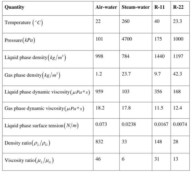
Table 2-1 : Comparison of the physical properties of two-phase mixtures of air-water, steam-water, Freon R-11 and Freon R-22 (Feenstra et al., 1995; Feenstra et al., 2002)

Quantity Air-water Steam-water R-11 R-22

Temperature

 

oC 22 260 40 23.3

Pressure



kPa



101 4700 175 1000

Liquid phase density



3



kg m 998 784 1440 1197

Gas phase density



kg m3



1.2 23.7 9.7 42.3

Liquid phase dynamic viscosity



Pa s*



959 103 356 168 Gas phase dynamic viscosity



Pa s*



18.2 17.8 11.5 12.4 Liquid phase surface tension



N m



0.073 0.0238 0.0167 0.0074

Density ratio



 _L _G



832 33 148 28

Viscosity ratio



 _L _G



46 6 31 13

2.2.5 Types of two-phase mixtures

A majority of flow-induced vibration studies have been conducted in single phase flow; gas or liquid. Additionally, most of the reported experimental studies in two-phase flow are done in air-water mixture, yet more than one-half of all steam generators operate in steam-air-water flow

(40)

(Pettigrew & Taylor, 1994). As is seen in Table 2-1, the main two phase parameters vary from mixture to mixture thus, raising the question of the applicability of the laboratory experimental results to prototypical steam generator operating conditions. To overcome this challenge, some studies (e.g. (Pettigrew et al., 1995), (Pettigrew & Taylor, 2009), (Feenstra et al., 1995) ) have used Freon due to the close proximity of its liquid/vapor density ratio to that of water/steam as is evident in Table 2-1. However, in the study reported in this report, air-water mixture is used. Recently, Sawadogo (2016) demonstrated that there is no significant difference in the critical velocity for fluidelastic instability of a rotated triangular tube array of P D 1.5 obtained with the array subjected to either two-phase Freon or air-water mixture.

2.3 Theoretical models for fluidelastic instability

As an aid to steam generator designers, ASME has recommended some design guidelines in the form of stability maps in which fluidelastic instability experimental data for different tube bundle geometrical configurations are plotted (Figure 2-5). A lower bound of this data is considered to be the stability threshold.

In as much as the design guideline has been an attempt to standardize steam generator production, it fails to provide information on the physics of the problem hence limits room for future improvements in steam generator design (Weaver, 2008). A number of models have been developed to predict the occurrence and improve understanding of the nature of the phenomenon of fluidelastic instability. These models are described in this section.

2.3.1 Jet-switch model

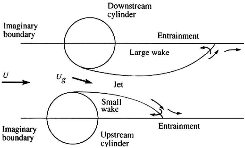
Roberts (1962, 1966) was the first to study self-excited oscillations of single and double row of cylinders subjected to cross-flow. His investigations showed that instability was primarily in the streamwise direction (at least for tube rows). Roberts (1962) considered the flow downstream of two adjacent cylinders to comprise two unequal wake regions supplied by a jet flow between them as illustrated in Figure 2-6.

(41)

19

Figure 2-5 : ASME fluidelastic instability design guideline map for heat exchangers (Weaver, D.S. & Fitzpatrick, J. A., 1988)

He contended that instability would occur if the jet-switching mechanism synchronized with tube motion in such a way that net energy was absorbed by the cylinder. Roberts developed a semi-empirical model relating the critical velocity,

 

U_c , for fluidelastic instability to the mass-damping parameter



m D2



in the following manner:

1 2 2 c n U m K D D            (2-22)

where _n,D, , m , , and K are the tube natural frequency, the outer diameter of the cylinder, the logarithmic decrement of damping, the mass per unit length , the ratio of fluidelastic frequency to structural frequency , the fluid density and a constant obtained from experiments, respectively.

Streamwise Fluidelastic Instability of Tube Arrays Subjected to Two-Phase Flow

ACKNOWLEDGEMENTS

RÉSUMÉ

ABSTRACT

TABLE OF CONTENTS

LIST OF TABLES

LIST OF FIGURES

 





LIST OF SYMBOLS AND ABBREVIATIONS

 

 

 

 

 

CHAPTER 1

INTRODUCTION

1.1 Objectives

1.2 Outline of the Thesis

CHAPTER 2

LITERATURE REVIEW

2.1 Flow induced excitation mechanisms

2.1.1 Turbulent buffeting

2.1.2 Vortex shedding and general flow periodicities













2.1.3 Fluidelastic instability

 

 

 

 

 

 

   

 

 

 

 

 

 

 

 

   





 



   



 



   



   

 

 

 





2.1.4 Streamwise fluidelastic instability





P D 

1.37

2.2 Two-phase flow induced vibrations

2.2.1 Two-phase flow models







 



2.2.2 Flow regimes

2.2.3 Added mass (hydrodynamic mass)



