Plasmapheric plumes: CLUSTER, image and simulations.

HAL Id: hal-00154293

https://hal.archives-ouvertes.fr/hal-00154293

HAL is a multi-disciplinary open access archive for the deposit and dissemination of sci-entific research documents, whether they are pub-lished or not. The documents may come from teaching and research institutions in France or abroad, or from public or private research centers.

L’archive ouverte pluridisciplinaire HAL, est destinée au dépôt et à la diffusion de documents scientifiques de niveau recherche, publiés ou non, émanant des établissements d’enseignement et de recherche français ou étrangers, des laboratoires publics ou privés.

Plasmapheric plumes: CLUSTER, image and

simulations.

F. Darrouzet, J. de Keyser, Pierrette Décréau, D. L. Gallagher, V. Pierrard, J.

F. Lemaire, B. R. Sandel, I. Dandouras, H. Matsui, M. Dunlop, et al.

To cite this version:

F. Darrouzet, J. de Keyser, Pierrette Décréau, D. L. Gallagher, V. Pierrard, et al.. Plasmapheric plumes: CLUSTER, image and simulations.. Proceedings Cluster and Double Star Symposium – 5th Anniversary of Cluster in Space. ESA SP-598, Sep 2005, Noordwijk, Netherlands. �hal-00154293�

Plasmapheric plumes: CLUSTER, image and simulations.

Some of the authors of this publication are also working on these related projects:

PICASSO View project

Auroral Plasma Physics View project Johan De Keyser

Royal Belgian Institute for Space Aeronomy

271PUBLICATIONS   3,400CITATIONS    SEE PROFILE Pierrette M. E. Décréau CNRS Orleans Campus 240PUBLICATIONS   4,057CITATIONS    SEE PROFILE Viviane Pierrard

Belgian Institute for Space Aeronomy

134PUBLICATIONS   2,779CITATIONS    SEE PROFILE

Joseph Fritz Lemaire

Université Catholique de Louvain - UCLouvain

238PUBLICATIONS   4,829CITATIONS    SEE PROFILE

All content following this page was uploaded by Joseph Fritz Lemaire on 25 February 2015. The user has requested enhancement of the downloaded file.

PLASMASPHERIC PLUMES: CLUSTER, IMAGE AND SIMULATIONS

F. Darrouzet(1), J. De Keyser(1), P. M. E. Décréau(2), D. L. Gallagher(3), V. Pierrard(1), J. F. Lemaire(1,4), B. R. Sandel(5), I. Dandouras(6), H. Matsui(7), M. Dunlop(8), J. Cabrera(4), A. Masson(9), P. Canu(10), J. G. Trotignon(2), J.

L. Rauch(2), and M. André(11) (1)

Belgian Institute for Space Aeronomy (IASB-BIRA), Brussels, Belgium

(2)

Laboratoire de Physique et Chimie de l'Environnement (LPCE), CNRS and University of Orléans, Orléans, France

(3)

Marshall Space Flight Center (MSFC), NASA, Huntsville, Alabama, USA

(4)

Center for Space Radiation (CSR), Louvain la Neuve, Belgium

(5)

Lunar and Planetary Laboratory (LPL), University of Arizona, Tucson, Arizona, USA

(6)

Centre d’Etude Spatiale des Rayonnements (CESR), CNRS, Toulouse, France

(7)

Space Science Center (SSC), University of New Hampshire, Durham, New Hampshire, USA

(8)

Rutherford Appleton Laboratory (RAL), Chilton, Didcot, Oxon, United Kingdom

(9)

Research and Scientific Support Department (RSSD), ESTEC-ESA, Noordwijk, The Netherlands

(10)

Centre d'étude des Environnements Terrestre et Planétaires (CETP), CNRS, Vélizy, France

(11)

Swedish Institute of Space Physics (IRFU), Uppsala division, Uppsala, Sweden

ABSTRACT

Plasmaspheric plumes have been routinely observed by the CLUSTER and IMAGE missions. CLUSTER provides high time resolution four-point measurements of the plasmasphere. Electron density is derived from the WHISPER sounder supplemented by data from the electric field instrument EFW. The EUV imager onboard IMAGE provides global images of the plasmasphere. We present coordinated observations of one plume event and numerical simulations for its formation based on the interchange instability mechanism. We compare several aspects of the plume motion as determined by different methods: (i) boundary velocity calculated from time delays of plume boundaries observed by WHISPER on all four spacecraft, (ii) ion velocity derived from the ion spectrometer CIS onboard CLUSTER, (iii) drift velocity measured by the electron drift instrument EDI onboard CLUSTER and (iv) global velocity determined from successive EUV images. These different methods consistently indicate that plasmaspheric plumes rotate around the Earth, with their foot fully co-rotating, but with their tip rotating slower and moving farther out.

1. INTRODUCTION

The plasmasphere is a toroidal region located in the Earth’s magnetosphere and populated by cold and dense ionospheric plasma [1]. Large-scale density structures have been observed in the Plasmasphere Boundary Layer, PLS [2]. These structures are usually connected to the main body of the plasmasphere, and extend outward. They have been called “plasmaspheric tails” in the past [3] but are now known as “plasmaspheric plumes” [4]. Such structures have been commonly observed by in-situ and ground-based measurements [5-7]. Recently, plumes have been routinely observed in

global plasmaspheric images by the IMAGE spacecraft [4,8-11]. Plumes have also been identified in in-situ measurements of the CLUSTER mission [12-16]. The formation of these plumes has been predicted on the basis of different models. One of the potential mechanisms is based on the interchange instability and a

Kp-dependent electric field model [17]. This model is

able to explain the formation of plasmaspheric plumes as a result of a short-time enhancement of geomagnetic activity (Kp increase) followed by a decrease [18].

The purpose of this paper is to report plasmaspheric plume observations by CLUSTER. These observations are compared with global images made by IMAGE, and with numerical simulations. After presenting the instrumentation and the methods of analysis in Sect. 2, one event is discussed in Sect. 3. Sect. 4 contains a summary and conclusions.

2. INSTRUMENTATION AND METHODS OF ANALYSIS

2.1 CLUSTER mission

The four CLUSTER spacecraft (C1, C2, C3, C4) cross the plasmasphere from the Southern to the Northern Hemisphere every 57 hours at perigee around 4 RE [19].

Each satellite contains 11 identical instruments. Data obtained from 5 of them are used in this paper.

WHISPER can unambiguously identify the electron plasma frequency Fpe (related to the electron density Ne

by: Fpe{kHz} ~ 9 [Ne{cm-3}]1/2) through its two modes

[20]. In active mode, the sounder analyses the pattern of resonances triggered in the medium by a radio pulse. This allows the identification of Fpe [21]. In passive

mode, the receiver monitors the natural plasma emissions in the frequency band 2-80 kHz. The local

_________________________________________________________________

Proceedings Cluster and Double Star Symposium – 5th _{Anniversary of Cluster in Space,}

Noordwijk, The Netherlands, 19 - 23 September 2005 (ESA SP-598, January 2006)

wave’s cut-off properties lead to an estimation of Fpe

[22]. Above this frequency range, EFW [23] is used to estimate Ne from the spacecraft potential Vsc, which is

the potential difference between the antenna probes and the spacecraft body [24-26]. In order to facilitate inter-comparison of the data, we choose to plot the density as a function of the equatorial distance Requat (in units of

Earth radii): the geocentric distance of the magnetic field line on which the spacecraft is located, measured at the geomagnetic equator, which is identified as the location along the field line where the magnetic field strength reaches a minimum. A magnetic field model is used that combines the internal model IGRF95 and the external model Tsyganenko-96 [27]. These models are computed with the UNILIB library (http://www.oma.be/ NEEDLE/unilib.php/).

CIS measures the complete three-dimensional distribution functions of the major ion species (H+_{, He}+_, He++ _{and O}+_{) with a time resolution of 4 seconds [28].} Its energy range extends as low as the spacecraft potential in RPA (Retarding Potential Analyser) mode (0.7-25 eV/q), which is available on C1, C3, and C4. EDI measures the electron drift velocity using artificially injected electron beams [29]. This instrument works on C1, C2, and C3. The data used in this study have been cleaned and smoothed [30].

The FGM magnetometer provides high time resolution (22.4 Hz in normal mode) magnetic field measurements from all four spacecraft with an accuracy of at least 0.1 nT [31]. The data have been time-averaged to provide a time resolution of 4 seconds.

2.2 IMAGE mission

The IMAGE (Imager for Magnetopause-to-Aurora Global Exploration) spacecraft was launched into a polar orbit with an apogee of 8.2 RE [32]. The Extreme

Ultraviolet (EUV) imager onboard IMAGE provides global images of the plasmasphere every 10 minutes with a spatial resolution of 0.1 RE [4]. It is an imaging

system, which detects the 30.4 nm sunlight resonantly scattered by the He+ _{ions in the plasmasphere.}

For better comparison with simulations, EUV images have been projected onto the dipole magnetic equatorial plane, by assigning to each pixel the minimum dipole L-shell along the line-of-sight (as EUV images are taken close to the Earth, a dipole magnetic field model can be used for low to moderate geomagnetic activity) [33-35]. The mapped signal is then converted to column abundance using estimates for the solar flux at 30.4 nm, based on the Solar2000 empirical solar irradiance model [36]. Finally, the column abundance is converted to pseudo-density by dividing by an estimate of the distance along the line of sight that contributes most to the image intensity at each location in the field of view [35]. Therefore the EUV images shown here give an equatorial distribution of He+ _{pseudo-density versus L} and Magnetic Local Time (MLT). The lower sensitivity

threshold of the EUV instrument has been estimated to be 40 ± 10 electrons cm-3_{, or 4-8 He}+ _{ions cm}-3 _if assuming a ratio He+_/H+ _{around 0.1-0.2 [34].}

2.3 Numerical simulation

In the frame of the interchange instability mechanism, the plasmapause is formed in the post-midnight MLT sector where and when the parallel components of the gravitational and centrifugal forces balance each other (the Zero Parallel Force (ZPF) surface [37]) [17,38,39]. The plasmapause is determined by the innermost equipotential surface tangent to the ZPF. Simulations show how this mechanism can lead to a plasmapause variable position, but also to the formation of plumes,

shoulders or notches [18,40]. The Kp-dependent E5D

electric field model is used in these simulations [41].

2.4 Velocities

To study the motion of plasmaspheric plumes, we use velocities determined from different techniques. The

electron drift velocity VD is measured by EDI. The H+

velocity VH is determined from the ion distribution

functions measured by CIS. The accuracy of the velocity measurements in the plumes is limited by the low particle counting statistics. A four-point technique is applied to the features identified in the electron density profiles at the inner and outer boundary (supposed to be locally planar) of the plumes. We determine the normal boundary velocity VN (assumed to be constant) with a time delay method, i.e. from individual spacecraft positions and times of the boundary crossings. We also compute the co-rotation velocity at the centre of mass of the four CLUSTER

spacecraft: VC = 2пR / (24×60×60), where R is the

distance from the spacecraft to the Earth’s rotation axis. To be able to compare the CLUSTER velocities between each other and with the IMAGE velocity, we project all the CLUSTER velocities on the Requat axis by

using the same magnetic field models as in the WHISPER density analysis. If we have a vector u determined at the centre of mass C of the four spacecraft, we consider a small displacement (of the order of 100 km) of this point C to M with the velocity

u. We determine the projection C’ of C along the

magnetic field line, until the magnetic field strength reaches a minimum. By doing the same analysis with the point M, we determine the velocity ueq in the magnetic equatorial plane. We obtain thus the following velocities: VD-eq, VH-eq, VN-eq, VC-eq.

An average radial velocity, VIO-eq, can be computed

from the displacement in Requat of a structure as seen

during in- and outbound passes, when the spacecraft remains approximately in the same MLT sector.

From IMAGE data, we determine the motion VE of

geometrically identified parts of the plume in successive EUV images equatorially projected.

3. OBSERVATIONS: 2 JUNE 2002 3.1 CLUSTER observations

This event is observed for small separation distance between the four CLUSTER spacecraft (around 150 km), in the dusk sector (18:00 MLT) and when the geomagnetic activity had a peak value of Kp = 4 in the

previous 24 hours. A very wide plume is seen in the inbound and outbound passes on all four spacecraft. The electron density profiles of the plume as determined

from WHISPER and EFW (for the part above 80 cm-3₎

are shown in Fig. 1. Both structures have the same overall shape, with more variability during the inbound crossing. This similar global structure leads to consider that the same plume is crossed by the spacecraft at South and North latitudes of the plasmasphere. The similarity of the four profiles suggests that the plume has not moved significantly over the 2 hours time period between the inbound and outbound crossings. This is confirmed by the equatorial normal boundary velocities VN-eq derived from the time profiles and shown on the

figure. These velocities are quite small for the inbound plume crossing. Note the higher values at the outer boundary than at the inner one. This is less than 50% of the co-rotation velocity, VC-eq, which is between 4.1 and

2.4 km/s. 5.5 6 6.5 7 7.5 8 8.5 9 101 102 103 R_equat(R_E) V = 1.5 km/sN-eq V = 0.9 km/sN-eq V = 0.7 km/sN-eq V = 4.1 km/sN-eq V = 4.2 km/sN-eq V = 0.6 km/sN-eq V = 2.0 km/sN-eq V = 1.4 km/sN-eq V = 3.6 km/sN-eq V = 0.7 km/sN-eq _{V = 0.5 km/s} N-eq C1 C2 C3 C4 N e (cm -3)

Fig. 1. CLUSTER electron density profiles as a function of Requat for the two plume crossings on 2 June 2002.

The lower four curves correspond to the inbound pass, the upper curves (shifted by a factor 10) to the outbound

pass. The magnitude of the normal boundary velocities

VN-eq derived from the time delays of different features

and projected onto the equatorial plane are indicated.

The inner edge of the plume shifts 0.5 RE in 75 minutes,

corresponding to VIO-eq = 0.7 ± 0.1 km/s. For the outer

edge, we find VIO-eq = 0.5 ± 0.1 km/s. This suggests that

the plume is thinner in the outbound pass in the Northern hemisphere than in the inbound one in the Southern hemisphere; its inner edge moves to a larger equatorial distance.

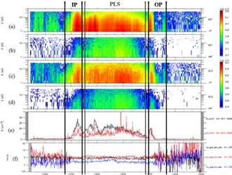
CIS data in RPA mode are shown on Fig. 2 for C1 and C3. The satellites enter the main plasmasphere at 12:45

UT and exit it at 13:55 UT, as indicated by the increase of ion populations (PLS region). The plumes are clearly seen in the H+ _{populations in the inbound pass between} 12:20 and 12:45 UT (IP region), and also in the outbound one between 14:00 and 14:20 UT (OP region).

IP PLS OP IP PLS OP

Fig. 2. CIS data: (a)-(b) distribution of H+ and He+ for C1; (c)-(d) same data for C3; (e) H+ density for C1 and

C3; (f) H+ velocity VH for C1 in GSE coordinates. The density values obtained from CIS are much lower than those determined from WHISPER, because of the limited energy range of the instrument in the RPA mode (0.7-25 eV/q). Inside the plasmasphere, the equatorially projected velocity VH-eq corresponds to the expected co-rotation orientation. But, during the inbound plume crossing, the Y component is higher, which means that the plume is probably moving away from the Earth. For the outbound plume pass no clear conclusions can be drawn as the trend is very different between C1 and C3. The drift velocity components determined by EDI during the inbound plume crossing are shown on panels (a) to (c) of Fig. 3 for C1, C2 and C3.

-10 -5 0 5 10 VD-eq YGSE (km/s) -10 -5 0 5 10 VD-eq ZGSE (km/s) -8 -4 0 4 8 VD-eq XGSE (km/s) C1 C2 C3 12:15 12:20 12:25 12:30 12:35 12:40 12:45 Time (UT) 0 40 80 120 Ne (cm -3) C1 C2 C3 C4 (a) (c) (b) (d)

Fig. 3. Inbound time profiles of (a)-(c) electron drift velocity VD-eq from EDI and projected onto the

equatorial plane; (d) electron density from WHISPER.

During this inbound crossing, the equatorially projected electron drift velocity is VD-eq = 1.7 ± 0.2 km/s (VXD-eq ~

-1.0 km/s, VY

D-eq ~ 1.3 km/s, VZD-eq ~ -0.5 km/s). This is

around 50% of the co-rotation velocity (3.3 km/s). The average direction of VD-eq is in the co-rotation direction; there is also a radial expansion of the plume (VY

D-eq >

0). During the outbound plume pass, VD-eq = 4.5 ± 0.2

km/s, opposite to the co-rotation direction, with a large

X component (VX

D-eq ~ 3.5 km/s, VYD-eq ~ 1.3 km/s,

VZ

D-eq ~ -2.5 km/s). This is consistent with the higher

values of the velocity determined from WHISPER in the outbound plume. Inside the plasmasphere (12:50-13:50 UT, i.e. Requat between 4.4 and 5.3 RE), VD-eq = 2.0 ± 0.2

km/s. Its magnitude and direction are close to the co-rotation velocity (2.1 ± 0.1 km/s).

3.2 IMAGE observations

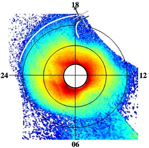
Fig. 4 presents an equatorially mapped EUV image at 12:33 UT, around the time of the inbound plume pass by CLUSTER. A very large plume (delimited by the white line) is observed in the post-dusk sector, with its foot attached to the plasmasphere between 17:30 and 22:00 MLT. At 17:30 MLT, it is located between 6.0 and 7.5 RE, which is consistent with the observations by

WHISPER, with a plume observed between 5.5 and 8.5

RE (but with an electron density above the estimated

EUV threshold only between 5.7 and 7.8 RE). The

normal directions computed from the time delay method applied to WHISPER data coincide approximately with that indicated by the global view from EUV.

24 18 12 06 24 18 12 06

Fig. 4. Equatorial projection of an EUV image at 12:33 UT. The white disk in the centre corresponds to the Earth. The big circles correspond to Requat = 3 and 5 RE.

The plume is delimited by the white line. The normal directions deduced with the time delay method for the inner and outer plume boundary crossings are shown by

the dark and light arrows respectively.

The plume is observed on EUV images from 10:10 UT until 14:30 UT. These successive images enable us to determine the motion of the plume. The foot of the plume (at 3.7 RE) moves at VE = 1.6 ± 0.1 km/s, close to

the co-rotation velocity VC-eq = 1.7 km/s. It is hard to

make the same calculation with the tip of the plume, which is difficult to identify unambiguously on the EUV images. From successive images, it can be seen that the tip is moving slower than the foot. EUV images show also that the tip is extending away from the Earth, consistent with CLUSTER showing the inner edge of the plume moving out from Requat = 5.5 to 6 RE.

3.3 Numerical simulations

Fig. 5 displays the plasmapause positions in the equatorial plane based on the Kp-dependent E5D electric

field model and on the interchange instability scenario.

(a) (b) (c) (d) B B→P P (a) (b) (c) (d)

1 June 2 June 3 June 4 June

(a) (b) (c) (d) B B→P P (a) (b) (c) (d)

1 June 2 June 3 June 4 June (a) (b) (c) (d)

1 June 2 June 3 June 4 June

Fig. 5. Predicted position of the plasmapause: top panel gives the solar wind and geomagnetic indices during the period of simulation (BBZ, Dst and Kp); bottom panels

indicate the plasmapause position and the evolution of a bulge (B) into a plume (P): (a) at 00:30 UT, (b) at

02:00 UT, (c) at 06:00 UT and (d) at 12:30 UT.

At the beginning of the simulation (panel a), the plasmapause is almost circular and located around 4.5

RE, but with a slight bulge (B) formed in the

post-midnight sector (panel b) after an increase of Kp up to 4

at 00:00 UT and the decrease of the Dst index (see top panel). This also corresponds to a southward turning of

the IMF BBZ. This bulge then evolves into a plume-like

structure (B→P), rotating around the Earth through all MLT sectors, at a velocity close to the co-rotation speed (panels c-d). At 12:30 UT the plume (P) is located in the dusk sector, between 17:00 and 18:00 MLT (panel d), and between 18:00 and 19:00 MLT at 14:15 UT. It is in the same local time sector where the CLUSTER spacecraft crossed the plume in the inbound (17:40-17:50 MLT) and outbound (18:15-18:30 MLT) passes. Comparing to the EUV image at 12:33 UT (Fig. 4), the plume is located between 18:00 and 22:00 MLT, but between 17:00 and 18:00 MLT in the simulation. This 1-3 hours shift can be explained by the poor time

resolution (only 3 hours) of the geomagnetic index Kp

used in the simulation. There is a good correlation between the simulated and observed plasmapause positions. In the morning sector, between 08:00 and 10:00 MLT, the simulation shows a plasmapause around

4 RE and the projected EUV image exhibits a

plasmapause between 4 and 4.5 RE. In the post-midnight

sector, it is located at 4.5 RE from the simulation, and

between 4.5 and 5 RE according to EUV observations.

It is interesting to notice that the plume is disappearing in the simulation around 23:00 UT, because Kp is still

increasing. Therefore the plasmapause is now forming closer to the Earth in the post-midnight sector, and the plume, as well as the outermost shell of the plasmasphere, are peeled off and convected away from the central core of the plasmasphere. On EUV images, the plume is also disappearing at the end of the day.

4. SUMMARY AND CONCLUSIONS

We have compared observations of plasmaspheric plumes by CLUSTER and IMAGE with numerical simulations. This study shows that the CLUSTER and IMAGE missions are complementary, because their different measurement techniques (global imaging and in-situ measurements) provide a more complete picture of plasmaspheric plumes.

The comparison between the global view from IMAGE and the in-situ measurements from CLUSTER gives consistent results concerning the position and size of the plumes. The plasmapause positions determined from WHISPER and EUV are consistent with the results predicted by the simulation code used in this article. The normal directions of the boundaries of the plumes as computed using the time delay method are consistent with EUV observations (see the projection of those normals on EUV image in Fig. 4).

The velocity analysis of the plumes gives consistent results between different techniques and different datasets. The main conclusion is that the plume is rotating around the Earth, with its foot attached to the main plasmasphere fully co-rotating, but with its tip rotating more slowly and moving outward, away from the Earth. This result is consistent with the topology of a plume, extending farther out at earlier MLT, as shown

in earlier studies [11,12]. Note that in the case studied here the plume is not moving inward, as might be expected from standard sunward MHD convection scenarios based on the enhancement of a uniform dawn-dusk convection electric field considered in earlier teardrop models of plasmasphere. As expected, the angular velocity of the inner edge of the plume is closer to co-rotation than the outer one.

The numerical simulation of the plasmapause positions

is based on McIlwain’s Kp-dependent empirical

magnetospheric electric field model E5D and on the interchange instability mechanism for the formation of the plasmapause. It reproduces rather well the formation and motion of the plasmaspheric plumes when the level of geomagnetic activity increases suddenly by sufficiently large step (ΔKp ≥ 2). Indeed, with a Kp in the

preceding 24 hours increasing suddenly from a small value to Kp > 3, a bulge is formed in the post-midnight

MLT sector, and develops subsequently into a plume while it co-rotates around the Earth into the dusk MLT sector. The comparison with the observations works well in terms of radial and MLT position of the plume. Some shifts in the simulated MLT positions are observed because of the 3 hours time resolution of the

Kp index used to modulate the E5D model. Note that

this model is an average quasi-static electric field model whose limitations may also explain some differences between the observations and the simulation [1,18]. To conclude, this study gives a global idea of the formation, evolution and motion of plasmaspheric plumes from three different datasets.

ACKNOWLEDGEMENTS

FD, JDK, and JL acknowledge the support by the Belgian Federal Science Policy Office through PRODEX-8/CLUSTER (contract 13127/98/NL/VJ(IC)).

REFERENCES

1. Lemaire J. F. and Gringauz K. I., The Earth's Plasmasphere, with contributions from D. L. Carpenter and V. Bassolo, Cambridge University Press, 372 pp., 1998.

2. Carpenter D. L. and Lemaire J., The Plasmasphere Boundary Layer, Ann. Geophys., 22, 4291–4298, 2004. 3. Taylor H. A. Jr., et al., Structured Variations of the Plasmapause, Evidence of a corotating plasma tail, J.

Geophys. Res., 76, 6806–6814, 1971.

4. Sandel B. R., et al., Initial Results from the IMAGE Extreme Ultraviolet Imager, Geophys. Res. Lett., 28, 1439–1442, 2001.

5. Chappell C. R., et al., The morphology of the bulge region of the plasmasphere, J. Geophys. Res., 75, 3848– 3861, 1970.

6. Foster J. C., et al., Ionospheric signatures of plasmaspheric tails, Geophys. Res. Lett., 29, doi:10.1029/2002GL015067, 2002.

7. Moldwin M. B., et al., Plasmaspheric plumes, CRRES observations of enhanced density beyond the plasmapause, J. Geophys. Res., 109, doi:10.1029/ 2003JA010320, 2004.

8. Sandel B. R., et al., Extreme ultraviolet imager observations of the structure and dynamics of the plasmasphere, Space Sci. Rev., 109, 25–46, 2003. 9. Garcia L. N., et al., Observations of the latitudinal structure of plasmaspheric convection plumes by IMAGE-RPI and EUV, J. Geophys. Res., 108, doi:10.1029/2002JA009496, 2003.

10. Goldstein J., et al., Simultaneous remote sensing and in situ observations of plasmaspheric drainage plumes,

J. Geophys. Res., 109, doi:10.1029/2003JA010281,

2004.

11. Spasojević M., et al., The link between a detached subauroral proton arc and a plasmaspheric plume,

Geophys. Res. Lett., 31, doi:10.1029/2003GL018389,

2004.

12. Darrouzet F., et al., Density structures inside the plasmasphere, Cluster observations, Ann. Geophys., 22, 2577–2585, 2004.

13. Darrouzet F., et al., Analysis of plasmaspheric plumes: CLUSTER and IMAGE observations and numerical simulations, Ann. Geophys., submitted, 2005. 14. Décréau P. M. E., et al., Observation of Continuum radiations from the CLUSTER fleet, first results from direction finding, Ann. Geophys., 22, 2607–2624, 2004. 15. Décréau P. M. E., et al., Density irregularities in the plasmasphere boundary player, Cluster observations in the dusk sector, Adv. Space Res., in press, 2005.

16. Dandouras I., et al., Multipoint observations of ionic structures in the Plasmasphere by CLUSTER-CIS and comparisons with IMAGE-EUV observations and with Model Simulations, Global Physics of the Coupled

Inner Magnetosphere (Proceedings of 2004 Yosemite

Workshop), in press, 2005.

17. Lemaire J. F., The formation plasmaspheric tails,

Phys. Chem. Earth (C), 25, 9–17, 2000.

18. Pierrard V. and Lemaire J. F., Development of shoulders and plumes in the frame of the interchange instability mechanism for plasmapause formation,

Geophys. Res. Lett., 31, doi:10.1029/2003GL018919,

2004.

19. Escoubet C. P., et al. (Eds.), The Cluster and Phoenix Missions, Kluwer Academic Publishers, 1997. 20. Décréau P. M. E., et al., Early results from the Whisper instrument on CLUSTER, an overview, Ann.

Geophys., 19, 1241–1258, 2001.

21. Trotignon J. G., et al., How to determine the thermal electron density and the magnetic field strength from the CLUSTER/WHISPER observations around the Earth,

Ann. Geophys., 19, 1711–1720, 2001.

22. Canu P., et al., Identification of natural plasma emissions observed close to the plasmapause by the Cluster-Whisper relaxation sounder, Ann. Geophys., 19, 1697–1709, 2001.

23. Gustafsson G., et al., First results of electric field and density observations by Cluster EFW based on

initial months of observations, Ann. Geophys., 19, 1219–1240, 2001.

24. Pedersen A., Solar wind and magnetosphere plasma diagnostics by spacecraft electrostatic potential measurements, Ann. Geophys., 13, 118–129, 1995. 25. Pedersen A., et al., Four-point high resolution information on electron densities by the electric field experiments (EFW) on Cluster, Ann. Geophys., 19, 1483–1489, 2001.

26. Moullard O., et al., Density modulated whistler mode emissions observed near the plasmapause,

Geophys. Res. Lett., 29, 10.1029/2002GL015101, 2002.

27. Tsyganenko N. A. and Stern D. P., Modeling the global magnetic field of the large-scale Birkeland current systems, J. Geophys. Res., 101, 27187–27198, 1996.

28. Rème H., et al., First multi-spacecraft ion measurements in and near the Earth's magnetosphere with the identical Cluster ion spectrometry (CIS) experiment, Ann. Geophys., 19, 1303–1354, 2001. 29. Paschmann, G., et al., The Electron Drift Instrument on Cluster, overview of first results, Ann. Geophys., 19, 1273–1288, 2001.

30. Matsui H., et al., Derivation of electric potential patterns in the inner magnetosphere from Cluster EDI data, Initial results, J. Geophys. Res., 109, doi:10.1029/ 2003JA010319, 2004.

31. Balogh A., et al., The Cluster Magnetic Field Investigation: overview of in-flight performance and initial results, Ann. Geophys., 19, 1207–1217, 2001. 32. Burch J. L., IMAGE mission overview, Space Sci.

Rev., 91, 1–14, 2000.

33. Roelof E. C. and Skinner A. J., Extraction of ion distributions from magnetospheric ENA and EUV images, Space Sci. Rev., 91, 437–459, 2000.

34. Goldstein J., et al., Identifying the plasmapause in IMAGE EUV data using IMAGE RPI in situ steep density gradients, J. Geophys. Res., 108, doi:10.1029/ 2002JA009475, 2003.

35. Gallagher D. L., et al., The origin and evolution of plasmaspheric notches, J. Geophys. Res., 110, doi:10.1029/2004JA010906, 2005.

36. Tobiska W. K., et al., The SOLAR2000 empirical solar irradiance model and forecast tool, J. Atmos. Terr.

Phys., 62, 1233–1250, 2000.

37. Lemaire J. F., Frontiers of the plasmasphere, Editions Cabay, Louvain-la-Neuve, ISBN 2-87077-310-2; Aeronomica Acta A 298, 1985.

38. Lemaire J. F., The ’Roche-limit’ of ionospheric plasma and the formation of the plasmapause, Planet.

Space Sci., 22, 757–766, 1974.

39. Lemaire J. F., The mechanisms of formation of the plasmapause, Ann. Geophys., 31, 175–190, 1975. 40. Pierrard V. and Cabrera J., Comparisons between EUV/IMAGE observations and numerical simulations of the plasmapause formation, Ann. Geophys., in press, 2005.

41. McIlwain C. E., A Kp dependent equatorial electric field model, Adv. Space Res., 6, 187–197, 1986.

View publication stats View publication stats