Université de Sherbrooke
Investigating local track geometry and its effects on water radiolysis using a new Monte Carlo method: Calculations of primary yields in relation to spatial
proximity between ionizing radiation tracks
Par Tait Du
Département de médecine nucléaire et radiobiologie
Mémoire présenté à la Faculté de médecine et des sciences de la santé en vue de l’obtention du diplôme de maître ès sciences (M.Sc.) en "sciences des radiations et imagerie biomédicale"
Sherbrooke, Québec, Canada February 2021
Jury
Pr Armand Soldera Examinateur, Département de chimie, Faculté des sciences
Pr Richard J. Wagner Examinateur, Département de médecine nucléaire et radiobiologie, Faculté de médecine et des sciences de la santé
Pr Jean-Paul Jay-Gerin Directeur de recherche, Département de médecine nucléaire et radiobiologie, Faculté de médecine et des sciences de la santé
ii
RÉSUMÉ
Étude de la géométrie locale des voies et de ses effets sur la radiolyse de l'eau à l'aide d'une nouvelle méthode de Monte-Carlo: Calculs des rendements primaires
en fonction de la proximité spatiale entre les traces de rayonnements ionisants Tait Du
Département de médecine nucléaire et radiobiologie
Mémoire présenté à la Faculté de médecine et des sciences de la santé en vue de l’obtention du diplôme de maître ès sciences (M.Sc.) en "sciences des radiations et imagerie biomédicale", Faculté
de médecine et des sciences de la santé, Université de Sherbrooke, Sherbrooke, Québec, Canada J1H 5N4
Dans ce travail, nous présentons les rendements simulés de diverses espèces radiolytiques résultant de traces d'ions incidents simultanés dans des conditions de proximité spatiale. Le code Monte-Carlo de la structure des traces de SHERBROOKE a été mis à jour afin de permettre le traitement de multiples traces d'ions simultanées à travers les étapes de la radiolyse. En utilisant une proximité spatiale variable, les rendements chimiques de deux traces d'ions parallèles et simultanées de TEL variable ont été calculés jusqu'à 1 µs. Pour toutes les traces d'ions incidentes, les rendements des espèces radicalaires, telles que le radical hydroxyle, sont réduits avec une proximité spatiale suffisante tandis que ceux des espèces moléculaires sont augmentés. Les rendements chimiques d'une seule trace d'ion à TEL élevé (ion carbone de 60 MeV) et de plusieurs traces à TEL faible (61 protons de 10 MeV) à faible proximité spatiale ont été simulés jusqu'à 1 ms. Les rendements des traces de protons à faible TEL sont étroitement liés à ceux des traces d'ions carbone à TEL élevé, en supposant qu'il n'y ait pas d'effets d'ionisations multiples. Les rendements de 9 trajectoires d'ions carbone de 1200 MeV ont été simulés avec deux configurations spatiales différentes dans le même volume. Avec la même énergie déposée dans le système, les configurations avec un chevauchement spatial élevé entre les trajectoires démontrent des rendements radicalaires plus faibles. Les rendements de 9 traces d'ions carbone de 1200 MeV, 49 traces de protons de 10 MeV et 676 traces de protons de 300 MeV ont été simulés dans le même volume dans le cadre d'un scénario de débit de dose élevé et de débit de dose ultra élevé. Avec la même énergie déposée dans le système, les traces de protons à faible TEL présentent un effet de proximité spatiale beaucoup plus important que les traces d'ions carbone à TEL élevé. Dans le contexte du domaine en pleine expansion des systèmes à débit de dose ultra-élevé comme l’ « effet FLASH » en radiothérapie, de tels effets de proximité spatiale sur les rendements radiolytiques peuvent avoir des impacts biologiques importants.
Mots-clés: Radiolyse de l'eau, transfert d'énergie linéaire (TEL), simulations Monte-Carlo, rendements radicalaires et moléculaires, proximité spatiale des traces d’ion.
iii
ABSTRACT
Investigating local track geometry and its effects on water radiolysis using a new Monte Carlo method: Calculations of primary yields in relation to spatial
proximity between ionizing radiation tracks Tait Du
Département de médecine nucléaire et radiobiologie
Thesis presented at the Faculty of Medicine and Health Sciences in order to obtain the Master of Sciences (M.Sc.) degree in “Radiation Sciences and Biomedical Imaging”, Faculty of Medicine and
Health Sciences, Université de Sherbrooke, Sherbrooke, Québec, Canada J1H 5N4
In this work we present the simulated yields of various radiolytic species under the conditions of simultaneous incident ion tracks being in spatial proximity. With the growing field of ultra-high dose rate schemes such as FLASH-RT, there is potential for spatial proximity-based effects on radiolytic yields having biological impacts. The SHERBROOKE track structure Monte Carlo code was used, and for the purposes of this work, have been updated to allow for the processing of multiple simultaneous ion tracks through the stages of radiolysis. Using varying spatial proximity, the chemical yields of two parallel and simultaneous ion tracks of varying LET have been calculated up to 1 microsecond. For all incident ion tracks, yields of radical species such as the hydroxyl radical are reduced with sufficient spatial proximity while those of molecular species are increased. The chemical yields of singular high LET ion track (60 MeV C6+)
and multiple low LET tracks (61 10 MeV protons) in close spatial proximity has been simulated up to 1 microsecond. The yields of the low LET proton tracks are closely related to that of the high LET carbon ion track assuming no multiple ionization effects. The yields of 9 1200 MeV C6+ ion tracks have been simulated with two different spatial
configurations in the same volume. With the same energy deposited in the system, the configuration with high spatial overlap between tracks demonstrates lower radical yields. The yields of 9 1200 MeV C6+ ion tracks, 49 10 MeV proton tracks, and 676 300
MeV proton tracks have been simulated in the same volume under a high dose rate and ultra high dose rate scenario. With the same energy deposited in the system, the low LET proton tracks demonstrated a much stronger spatial proximity effect than the high LET carbon ion tracks.
Keywords: Water radiolysis, linear energy transfer (LET), dose rate, Monte Carlo simulations, radical and molecular yields, ion track proximity.
iv Table of Contents Résumé ... ii Abstract ... iii Table of contents ... iv List of Tables ... vi
List of Figures ... vii
List of Abbreviations ... xii
1. Introduction ... 1
1.1 Radiation and its interaction with matter ... 1
1.2 FLASH overview ... 4
1.3 LET and track structure ... 7
1.3.1 Track structure in relation to LET ... 8
1.3.2 Low LET radiation ... 8
1.3.3 High LET radiation ... 11
1.3.4 Track proximity: Strength in numbers? ... 14
1.4 Radiolysis of water ... 15
1.4.1 Physical stage ... 16
1.4.2 Physico-chemical stage ... 17
1.4.3 Chemical stage ... 20
1.4.4 Biological implications following radiolysis ... 21
v
2. Methods ... 25
2.1 Monte Carlo ... 25
2.1.1 IONLYS ... 27
2.1.2 IRT ... 31
2.2 Changes made to the new SHERBROOKE code ... 36
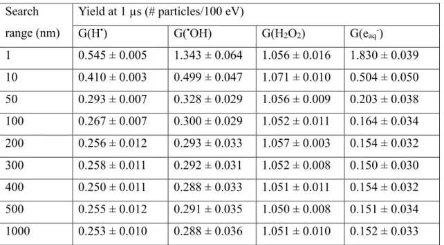
2.2.1 Optimal search ranges ... 39
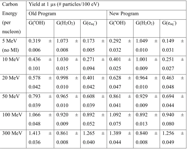
2.2.2 Comparability between old and new SHERBROOKE code ... 42
3. Results and discussion ... 46
3.1 Strength of the proximity effect ... 47
3.2 Effectiveness of multiple low LET tracks in mimicking a high LET track ... 57
3.3 Grid vs Hex ... 60
3.4 Does the geometrical beam arrangement have an effect? ... 64
3.5 Spatial proximity effect for the same dose of high LET and low LET radiation . ... 71
3.6 Future work ... 80
4. Conclusion ... 82
5. Acknowledgements ... 84
vi LIST OF TABLES
Chapter 2: Methodology
Table 2.1: Yields of chemical species produced at 1 µs by a 5 MeV carbon ion track (~284.4 keV/µm) with varying search ranges using the old and new SHERBROOKE code. ... 41 Table 2.2: Yields of chemical species produced at 1 µs by a 300 MeV proton track (~0.4 keV/µm) with varying search ranges using the old and new SHERBROOKE code. ... 41 Table 2.3: Yields of chemical species produced at 1 µs by a carbon ion track with varying initial energies using the old and new SHERBROOKE code. ... 43 Chapter 3: Results and discussion
Table 3.1: Yields at 1 µs generated by two parallel 300 MeV proton tracks (~0.4 keV/ μm) with varying distance between tracks. ΔG∞ represents the relative difference between yields at 1 µs
between Δx = 0 and Δx = “∞”. Confidence interval of 95%. ... 48 Table 3.2: Yields at 1 µs generated by two parallel 10 MeV proton tracks (~4.5 keV/ μm) with varying distance between tracks. ΔG∞ represents the relative difference between yields at 1 µs
between Δx = 0 and Δx = “∞”. Confidence interval of 95%. ... 51 Table 3.3: Yields at 1 µs generated by two parallel 60 MeV carbon ion tracks (~284.4 keV/ μm) with varying distance between tracks. ΔG∞ represents the relative difference between yields at 1 µs
between Δx = 0 and Δx = “∞”. Confidence interval of 95%. ... 54 Table 3.4: Yields at 1 µs generated by nine parallel 1200 MeV carbon tracks (~24.5 keV/μm), forty-nine parallel 10 MeV proton tracks, and six-hundred-and-seventy-six parallel 300 MeV proton tracks starting in a 100 nm by 100 nm square. The tracks are arranged in a square grid with 50 nm spacing between nearest tracks for the 1200 MeV carbon tracks, 16.7 nm spacing between nearest tracks for the 10 MeV proton tracks, and 4 nm spacing between nearest tracks for the 300 MeV proton tracks. The value in parenthesis denotes the yield generated with no spatial proximity effects. Confidence interval of 95%. ... 72 Table 3.5: Yields at 1 µs generated by nine parallel 1200 MeV carbon tracks (~24.5 keV/μm), forty-nine parallel 10 MeV proton tracks, and six-hundred-and-seventy-six parallel 300 MeV proton tracks starting in a 1 µm by 1 µm square. The tracks are arranged in a square grid with 500 nm spacing between nearest tracks for the 1200 MeV carbon tracks, 167 nm spacing between nearest tracks for the 10 MeV proton tracks, and 40 nm spacing between nearest tracks for the 300 MeV proton tracks. The value in parenthesis denotes the yield generated with no spatial proximity effects. Confidence interval of 95%. ... 76
vii LIST OF FIGURES
Chapter 1: Introduction
Figure 1.1: Track structure associated with low LET tracks. Track entities are denoted as “spurs” (spherical entities up to 100 eV), blobs (spherical or ellipsoidal, 100-500 eV) and short tracks (cylindrical, 500 eV- 5 keV) for a primary high energy electron (not to scale) (adapted from Burton, 1969). ... 10 Figure 1.2: Spatial location of radiolytic species post-energy deposition from the Monte Carlo track simulation of 300 MeV protons (A) and 150 keV protons (B) (LET~ 0.4 and 70 keV/µm) incident on liquid water at 25 °C. ... 11 Figure 1.3: Track structure and associated primary energy-loss events in high LET tracks. (adapted from Ferradini, 1979). ... 12 Figure 1.4: Spatial location of radiolytic species post-energy deposition from the Monte Carlo track simulation of 150 keV protons (A), 7 MeV alpha particles (B), and 306 MeV carbon ions (C) incident on liquid water at 25 °C. Incident radiation was chosen such that the LET of the tracks
would be the same (~70 keV/µm). ... 13 Figure 1.5: Time scale of events in the radiolysis of pure, deaerated water using low LET radiation. (Meesungnoen, 2007; Meesungnoen and Jay-Gerin, 2010) The different colors used are for visual clarity to highlight the individual processes that occur during radiolysis. ... 16 Chapter 2: Methodology
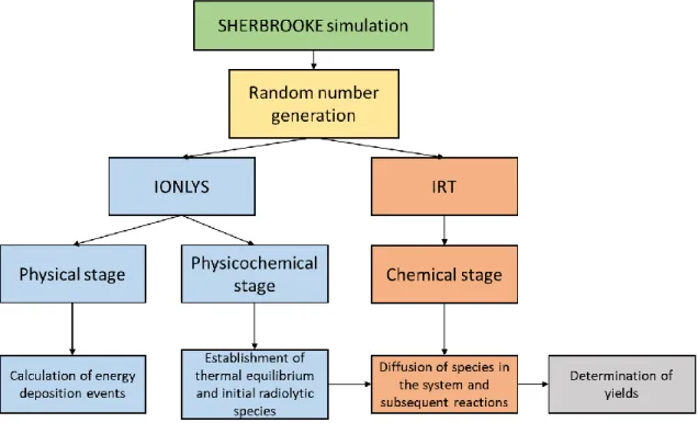
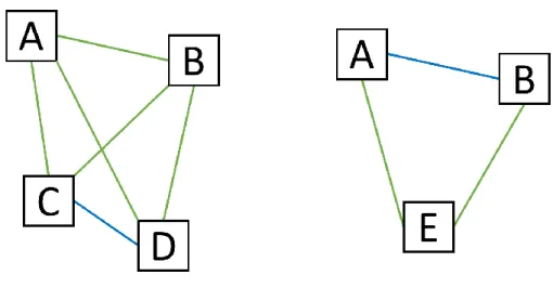
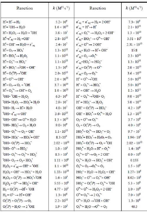
Figure 2.1: Schematic for the basic operation of the SHERBROOKE code. ... 27 Figure 2.2: Schematic for the principles behind the IRT method. On the left are particles A, B, C, and D where the green lines between particles/boxes represents a possible reaction between particles while the blue line represents the fastest reaction. On the right we show the results after the reaction of particles C and D which has generated a new particle E. ... 33 Figure 2.3: Reaction scheme and associated rate constants (k) for the radiolysis of pure water at 25 ⃘C.
(Meesungnoen and Jay-Gerin, 2011) Some rate constants have been updated using data from Elliot and Bartels (2009). ... 35 Figure 2.4: Comparison between an ordered array (left) and an ordered linked list (right) when inserting a new particle. For the array, the insertion of the new particle destroys the ordering while for the linked list, the ordering is preserved. ... 39
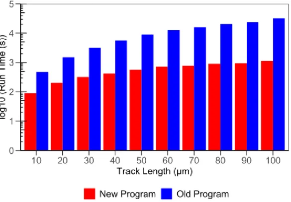
viii Figure 2.5: Runtime needed to calculate yields up to 1 µs for singular carbon ion tracks using the old and new SHERBROOKE code with initial carbon ion energy fixed to 1200 MeV (~24.5 keV/μm) with varying track lengths ... 45 Figure 2.6: Runtime needed to calculate yields up to 1 µs for singular carbon ion tracks using the old and new SHERBROOKE code with track length fixed at 50 µm with varying initial carbon ion energies. ... 45 Chapter 3: Results and discussion
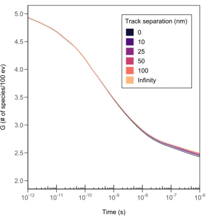
Figure 3.1: Comparison of time dependent yields of •OH generated by two parallel 300 MeV proton
tracks (~0.4 keV/ μm) at 1 µs with varying distance between tracks. ... 49 Figure 3.2: Comparison of time dependent yields of H2O2 generated by two parallel 300 MeV
proton tracks (~0.4 keV/ μm) at 1 µs with varying distance between tracks. ... 49 Figure 3.3: Comparison of time dependent yields of eaq- generated by two parallel 300 MeV proton
tracks (~0.4 keV/ μm) at 1 µs with varying distance between tracks. ... 50 Figure 3.4: Comparison of time dependent yields of •OH generated by two parallel 10 MeV proton
tracks (~4.5 keV/ μm) at 1 µs with varying distance between tracks. ... 52 Figure 3.5: Comparison of time dependent yields of H2O2 generated by two parallel 10 MeV proton
tracks (~4.5 keV/ μm) at 1 µs with varying distance between tracks. ... 52 Figure 3.6: Comparison of time dependent yields of eaq- generated by two parallel 10 MeV proton
tracks (~4.5 keV/ μm) with varying distance between tracks. ... 53 Figure 3.7: Comparison of time dependent yields of •OH generated by two parallel 60 MeV carbon
ion tracks (~284.4 keV/ μm) at 1 µs with varying distance between tracks. ... 55 Figure 3.8: Comparison of time dependent yields of H2O2 generated by two parallel 60 MeV carbon
ion tracks (~284.4 keV/ μm) at 1 µs with varying distance between tracks. ... 55 Figure 3.9: Comparison of time dependent yields of eaq- generated by two parallel 60 MeV carbon
ion tracks (~284.4 keV/ μm) with varying distance between tracks. ... 56 Figure 3.10: Comparison of time dependent yields of •OH generated by sixty-one superimposed 10
MeV proton tracks (~4.5 keV/μm), one 60 MeV carbon ion track (~284.4 keV/μm) with and without multiple ionization, and one 10 MeV proton track. ... 58
ix Figure 3.11: Comparison of time dependent yields of H2O2 generated by sixty-one superimposed 10
MeV proton tracks (~4.5 keV/μm), one 60 MeV carbon ion track (~284.4 keV/μm) with and without multiple ionization, and one 10 MeV proton track. ... 59 Figure 3.12: Comparison of time dependent yields of eaq- generated by sixty-one superimposed 10
MeV proton tracks (~4.5 keV/μm), one 60 MeV carbon ion track (~284.4 keV/μm) with and without multiple ionization, and one 10 MeV proton track. ... 59 Figure 3.13: Basic geometry of a square grid (left) and hexagonal grid (right). The red circle denotes the “central” vertex, with the green circles denoting the closest vertices to the central vertex, and the blue circles denoting the second closest vertices to the central vertex. s represents the side length of the square or hexagonal constituents of the grid. ... 61 Figure 3.14: Comparison of time dependent yields of •OH generated by twenty-five parallel 10 MeV
proton tracks (~4.5 keV/μm) in two configurations. The first configuration has the proton tracks arranged in a 5 x 5 square grid with 10 nm side length, and the second configuration has the proton tracks arranged in a hexagonal grid with 10 nm side length. ... 62 Figure 3.15: Comparison of time dependent yields of H2O2 generated by twenty-five parallel 10
MeV proton tracks (~4.5 keV/μm) in two configurations. The first configuration has the proton tracks arranged in a 5 x 5 square grid with 10 nm side length, and the second configuration has the proton tracks arranged in a hexagonal grid with 10 nm side length. ... 63 Figure 3.16: Comparison of time dependent yields of eaq- generated by twenty-five parallel 10 MeV
proton tracks (~4.5 keV/μm) in two configurations. The first configuration has the proton tracks arranged in a 5 x 5 square grid with 10 nm side length, and the second configuration has the proton tracks arranged in a hexagonal grid with 10 nm side length. ... 64 Figure 3.17: Comparison of time dependent yields of •OH generated by nine parallel 1200 MeV
carbon tracks (~24.5 keV/μm) in two configurations. The first configuration has the carbon ion tracks arranged in a 3 x 3 square grid with 50 nm spacing between tracks, and the second configuration has the carbon ion tracks located on the cardinal directions relocated so that each corner has 2 tracks. ... 66
x Figure 3.18: Comparison of time dependent yields ofH2O2 generated by nine parallel 1200 MeV
carbon tracks (~24.5 keV/μm) in two configurations. The first configuration has the carbon ion tracks arranged in a 3 x 3 square grid with 50 nm spacing between tracks, and the second configuration has the carbon ion tracks located on the cardinal directions relocated so that each corner has 2 tracks. ... 67 Figure 3.19: Comparison of time dependent yields of eaq- generated by nine parallel 1200 MeV
carbon tracks (~24.5 keV/μm) in two configurations. The first configuration has the carbon ion tracks arranged in a 3 x 3 square grid with 50 nm spacing between tracks, and the second configuration has the carbon ion tracks located on the cardinal directions relocated so that each corner has 2 tracks. ... 68 Figure 3.20: Comparison of time dependent yields of •OH generated by nine parallel 1200 MeV
carbon tracks (~24.5 keV/μm) in two configurations. The first configuration has the carbon ion tracks arranged in a 3 x 3 square grid with 500 nm spacing between tracks, and the second configuration has the carbon ion tracks located on the cardinal directions relocated so that each corner has 2 tracks. ... 69 Figure 3.21: Comparison of time dependent yields of H2O2 generated by nine parallel 1200 MeV
carbon tracks (~24.5 keV/μm) in two configurations. The first configuration has the carbon ion tracks arranged in a 3 x 3 square grid with 500 nm spacing between tracks, and the second configuration has the carbon ion tracks located on the cardinal directions relocated so that each corner has 2 tracks. ... 70 Figure 3.22: Comparison of time dependent yields of eaq- generated by nine parallel 1200 MeV
carbon tracks (~24.5 keV/μm) in two configurations. The first configuration has the carbon ion tracks arranged in a 3 x 3 square grid with 500 nm spacing between tracks, and the second configuration has the carbon ion tracks located on the cardinal directions relocated so that each corner has 2 tracks. ... 71 Figure 3.23: Comparison of time dependent yields of •OH generated by nine parallel 1200 MeV
carbon tracks (~24.5 keV/μm), forty-nine parallel 10 MeV proton tracks, and six-hundred-and-seventy-six parallel 300 MeV proton tracks starting in a 100 nm by 100 nm square. The tracks are arranged in a square grid with 50 nm spacing between nearest tracks for the 1200 MeV carbon tracks, 16.7 nm spacing between nearest tracks for the 10 MeV proton tracks, and 4 nm spacing between nearest tracks for the 300 MeV proton tracks. ... 73
xi Figure 3.24: Comparison of time dependent yields of H2O2 generated by nine parallel 1200 MeV
carbon tracks (~24.5 keV/μm), forty-nine parallel 10 MeV proton tracks, and six-hundred-and-seventy-six parallel 300 MeV proton tracks starting in a 100 nm by 100 nm square. The tracks are arranged in a square grid with 50 nm spacing between nearest tracks for the 1200 MeV carbon tracks, 16.7 nm spacing between nearest tracks for the 10 MeV proton tracks, and 4 nm spacing between nearest tracks for the 300 MeV proton tracks. ... 74 Figure 3.25: Comparison of time dependent yields of eaq- generated by nine parallel 1200 MeV
carbon tracks (~24.5 keV/μm), forty-nine parallel 10 MeV proton tracks, and six-hundred-and-seventy-six parallel 300 MeV proton tracks starting in a 100 nm by 100 nm square. The tracks are arranged in a square grid with 50 nm spacing between nearest tracks for the 1200 MeV carbon tracks, 16.7 nm spacing between nearest tracks for the 10 MeV proton tracks, and 4 nm spacing between nearest tracks for the 300 MeV proton tracks. ... 75 Figure 3.26: Comparison of time dependent yields of •OH generated by nine parallel 1200 MeV
carbon tracks (~24.5 keV/μm), forty-nine parallel 10 MeV proton tracks, and six-hundred-and-seventy-six parallel 300 MeV proton tracks starting in a 100 nm by 100 nm square. The tracks are arranged in a square grid with 500 nm spacing between nearest tracks for the 1200 MeV carbon tracks, 167 nm spacing between nearest tracks for the 10 MeV proton tracks, and 40 nm spacing between nearest tracks for the 300 MeV proton tracks. ... 77 Figure 3.27: Comparison of time dependent yields of H2O2 generated by nine parallel 1200 MeV
carbon tracks (~24.5 keV/μm), forty-nine parallel 10 MeV proton tracks, and six-hundred-and-seventy-six parallel 300 MeV proton tracks starting in a 100 nm by 100 nm square. The tracks are arranged in a square grid with 500 nm spacing between nearest tracks for the 1200 MeV carbon tracks, 167 nm spacing between nearest tracks for the 10 MeV proton tracks, and 40 nm spacing between nearest tracks for the 300 MeV proton tracks. ... 78 Figure 3.28: Comparison of time dependent yields of eaq- generated by nine parallel 1200 MeV
carbon tracks (~24.5 keV/μm), forty-nine parallel 10 MeV proton tracks, and six-hundred-and-seventy-six parallel 300 MeV proton tracks starting in a 100 nm by 100 nm square. The tracks are arranged in a square grid with 500 nm spacing between nearest tracks for the 1200 MeV carbon tracks, 167 nm spacing between nearest tracks for the 10 MeV proton tracks, and 40 nm spacing between nearest tracks for the 300 MeV proton tracks. ... 79
xii
LIST OF ABBREVIATIONS
D Diffusion coefficient
DEA Dissociative electron attachment
DNA Deoxyribonucleic acid
e−aq Hydrated electron
eV Electron-volt
GX or g(X) Primary yield of the radiolytic species X
G(X) Experimental yield of the final product X
Gy/s Gray/second (dose rate)
IRT Independent reaction times
k Reaction rate constant
keV Kilo-electron-Volts
LET Linear energy transfer
MC Monte Carlo MeV Mega-electron-Volts µm Micrometer µs Microsecond ps Picosecond ∆G Yields variation
1
1. Introduction
1.1 Radiation and its interaction with matter
The term radiation is used to describe the phenomena of energy being emitted or transmitted through space or some other media in the form of particles or as waves. Described over one hundred years ago in 1895 with the discovery of X-rays by Wilhelm Conrad Röntgen, research into the phenomena of radiation and subsequently radioactive materials rapidly progressed in the following years with the discovery of the radioactivity of uranium by Henri Becquerel and of polonium and radium by Marie Curie and Pierre Curie. It quickly became evident with observation of the evolution of hydrogen and oxygen from a solution of water and radium salts by Marie Curie and André-Louis Debierne in 1901 that the interaction between water and radiation would be of high importance. This study of water’s chemistry when exposed to radiation would quickly encompass research into what intermediate species are produced and their subsequent time-evolution, the possible chemical reactions that can occur between those species, as well as the yields of said species. In particular, the invention of more sophisticated X-ray machines in the 1930s would be a turning point for the study of the interaction of water and radiation, as increased usage of X-rays in medical applications led to concerns about the biological impacts of radiation on the human body which is primarily composed of water.
The advent of the harnessing of nuclear fission in the mid-forties during World War II led to an explosive increase in radiochemistry. While some of this was driven via the need to convert the energy generated by nuclear fission into a usable form, much of the research was driven towards the study and subsequent prevention of undesirable effects or damages caused by radiation. With more readily available sources for radioisotopes being present, there was also increasing interest into new medical treatments utilizing radiation. This need to understand the physical and subsequent
2
chemical processes that ionizing radiation undergoes through the human body are key to understanding the future biological impacts. Though ionizing radiation fundamentally acts similarly in all mediums, the properties of the medium affect the overall chemistry that occurs. For safe usage in biological systems, a number of factors must be considered, ranging from the types of species produced and their relevant spatial distributions, to the reactions that can occur between said species. (Jonah, 1995). Understanding the behavior of simpler systems such as liquid water when exposed to radiation is necessary for understanding more complex biological systems, such as living cells that are composed primarily of water.
Over the course of the last century, the radiation chemistry of water has been well established. In the liquid phase of water, interactions with radiation primarily produce H•, H
2, H+, eaq-, H2O2, •OH, OH-, and HO2•. For biological systems, although
there are instances of “direct” damage incurred via direct absorption of energy from ionizing radiation to the various biological constituents of cells which disrupts their function, such as in DNA, there are also damages attributable to “indirect” effects. Depending on the location of the biological constituent being targeted, the ratio of indirect to direct damages is typically 70:30, however for some more concentrated macromolecules such as DNA located in the nucleus, this ratio skews more towards 50:50. These “indirect” effects arise from the radiolytic species produced from the water molecules in the cell, which can then undergo chemical reactions with other radiolytic species or the biological constituents of the cells themselves. (Azzam et al., 2012; Muroya et al., 2006; Nathan, 2003; Forman et al., 2004; Veal et al., 2007) An example of this would be extremely reactive •OH radicals that can rapidly undergo
reactions with other radiolytic species in the system to form species such as H2O2 or
react directly with DNA. Thus, to understand the biological impacts of the radiation chemistry of water, the production and subsequent reactions of radiolytic species must
3
be accurately predicted in relation to the ionizing radiation that is used.
Naturally, the amount of energy absorbed by the medium from the ionizing radiation plays a major role in the radiation chemistry of the system. Typically denoted by the gray or Gy (J/kg), the “dose” is the unit used to represent the amount of energy the ionizing radiation has deposited in the medium. Luckily for our purposes, dose calculations on aqueous solutions comprised mostly of light-weight molecules (i.e. water) will closely mimic that of biological tissue. (Stenström and Lohmann, 1933) The dose of a particular regime of ionizing radiation can be attributed to a number of factors including the linear energy transfer (LET) of the ionizing radiation, the flux of the ionizing radiation, and how long the ionizing radiation is applied to the system. Naturally, while the overall dose does play a role in the radiation chemistry of the system, there is a considerable difference between large doses applied over very long time periods and those applied over very short time periods. (Favaudon et al., 2014) In particular, we typically denote the “dose rate”, which is the dose applied to the system per unit time as Gy/s, or Sv/s, when calculating the dose rate for biological systems. As the Earth is inundated with both natural and artificial sources of radiation, there is essentially a background dose rate that terrestrial organisms must endure, where cellular mechanisms have been developed in order to repair damage caused by ionizing radiation or other processes over time to structures like DNA. (von Sonntag, 2006) Thus, in order to employ ionizing radiation for the destruction of targeted cells such as cancer cells, a sufficiently high dose rate has to be applied to the targeted cells such that it overwhelms any sort of repair mechanism. Conventionally, this dose rate is less than 0.03 Gy/s which is applied over many sessions to allow for the destruction of cancer cells while sparing healthy cells that are more capable of repairing themselves between sessions compared to cancer cells. (Withers, 1975)
4
1.2 FLASH overview
A new development in radiotherapy has been the use of extremely high dose rates such as FLASH-RT, first named by Favaudon et al. in 2014, where the mean dose rate can exceed 100 Gy/s. The exact delivery system for FLASH-RT varies depending on the delivered radiation type, but we can characterize the ideal delivery as a total dose above 10 Gy delivered in a timeframe of less than 0.1 s. (Vozenin et al., 2019a) The mean dose rate across pulses is greater than 100 Gy/s, however, dose rates can exceed 106 Gy/s within pulses of radiation. While the usage of high dose rates has been
described since the 1960s, (Wilson J.D. et al, 2020) Favaudon et al. recently popularized the field with their study on the thoracic irradiation of mice using conventional and FLASH dose rates. (Favaudon et al., 2014) In particular, their study showed that when a single 17 Gy dose was applied at conventional rates (0.03 Gy/s), mice experienced pulmonary fibrosis as early as 8 weeks after irradiation with major damages occurring 24 weeks after irradiation, whereas the same dose applied with FLASH-RT (>40 Gy/s) resulted in significantly less pulmonary fibrosis even following 24 weeks after irradiation. It was found that a significantly higher dose of 30 Gy was necessary for mice exposed to FLASH-RT to exhibit the same pulmonary fibrosis response as conventional radiotherapy. This “sparing” effect on normal tissue by FLASH-RT has been exhibited on a number of tissue types in different animal models which demonstrates the robustness of the effect. (Vozenin et al., 2019a; Vozenin et al., 2019b; Girdhani et al., 2019; Montay-Gruel et al., 2017; Montay-Gruel et al., 2019) Of course, sparing normal tissue does not mean much for radiotherapy if the tumor response to FLASH-RT is also negligible. However, studies using human xenografts (breast cancer, head/neck carcinoma) grafted on mice demonstrated that FLASH-RT has a similar tumor response as conventional radiotherapy. (Fauvadon et al., 2014) The effects of FLASH-RT has been demonstrated using various ionizing radiation, including
5
electrons (Favaudon et al., 2014), X-rays (Montay-Gruel et al., 2018), and protons (Girdhani et al., 2019) thus far, with the caveats that the presence of the FLASH effect seems to be heavily influenced by the combination of mean dose rate, total dose, radiation source, the pulse frequency of the radiation source, or other biological factors. (Wilson J.D. et al, 2020; Venkatesulu et al., 2019) While research into the tumor response to FLASH-RT is still in its infancy, results from different tissue and animal models have been promising.
There is a slight issue in that while there has been significant study in how FLASH-RT could have clinical benefits, it is still unclear how the FLASH-RT effects manifest themselves. FLASH-RT can be postulated to diverge from conventional RT from a very early stage of radiolysis, as each dosage of FLASH-RT could be entirely deposited within the timeframe of “heterogeneous” chemistry. The most prominent explanation thus far for the FLASH effect is the local depletion of oxygen in the exposed tissues which generates an extremely short period of hypoxia. (Adrian et al. 2020) The relationship between oxygen depletion and high dose rates has been explored in the past by Dewey and Boag (Dewey and Boag, 1959) who showed that bacteria irradiated by ultra-high dose rate radiation had similar survival rates to bacteria in a hypoxic environment, as well as having a better survival rate than bacteria exposed to conventional dose rates. They proposed that the ultra-high dose rate effectively depleted the local oxygen before any oxygen from surrounding tissues could diffuse and replenish the oxygen in the irradiated tissue. As healthy tissue typically retains higher oxygen concentrations than tumors, the usage of ultra-high dose rates or FLASH to deplete the local oxygen is proposed to generate a short period of radioresistance in healthy tissue. This “sparing” effect on healthy tissue and its reliance on local oxygen concentration has been examined via the irradiation of mouse brains, where it was observed that increasing the local oxygen concentration via carbogen breathing
6
nullified the cognitive protection provided by FLASH-RT. (Montay-Gruel et al., 2019) In theory this “sparing” effect should also be present for tumors, yet FLASH-RT is still shown to maintain similar or better tumor response compared to conventional methods. One proposed explanation is that because FLASH-RT essentially instantaneously produces large amounts of free radicals, the resulting difference between healthy tissues and cancerous tissue in their ability to process said free radicals results in the tumor responding more readily to FLASH. (Vozenin et al., 2019; Spitz et al., 2019) The lingering free radicals and other reactive species in the tumor then promote oxidative injuries or death. Thus, the FLASH effect likely relies on the differential of the removal of reactive species generated by radiolysis between healthy tissue and tumor tissue.
FLASH-RT still remains in its infancy as the equipment needed to demonstrate the FLASH effect is not yet fully developed for the clinical stage. While waiting for multimillion-dollar requests for new equipment to be accepted, there are other questions about FLASH-RT that need to be answered. Of particular concern is the initial radiochemistry that follows shortly after irradiation. FLASH-RT shortens the period in which ionization events occur from hundreds or thousands of seconds to a fraction of a second, implying that orders of magnitude more ionization events occur within a close spatial and temporal proximity compared to conventional radiation sources. This should lead to vastly different outcomes in terms of the amounts of the various radiolytic species that are generated and their half-lives, as reaction pathways that are not as prevalent with conventional dose rates would be more common with the density of radiolytic species. As the production of reactive species such as free radicals or hydroperoxides is of utmost importance in radiotherapy, being capable of describing the early stages of radiolysis following ultra-high dose rates of ionizing radiation is necessary for fully understanding the capabilities of FLASH-RT. To this end, we have devised modifications to our research group’s existing water radiolysis simulation
7
system to allow for the study of ultra-high dose rates in water radiolysis. 1.3 LET and track structure
When traveling through some medium, ionizing radiation does not instantaneously deposit all of its energy into the nearest molecule, but instead loses energy via many collisions along its path. Thus to understand the interaction between ionizing radiation and the medium it is traveling through, we must account for both the total energy deposited into the medium as well as the spatial distribution of energy deposition events. A simplified version of this concept known as the “linear energy transfer” (LET) or “stopping power” is the measure of how much energy is lost per unit path length by an ionizing particle traveling through some medium as demonstrated by the following formula: (Danzker et al., 1959)
𝐿𝐸𝑇 =−𝑑𝐸
𝑑𝑥 (1.1)
Here dE represents average energy deposited in the vicinity of the particle track transferred by the particle traveling a distance dx. (ICRU Report 16, 1970) Typically, the LET is reported in units of keV per micrometer (keV/µm). The LET can be attributed to both the ionizing radiation used, as well as the medium that it travels through. For the ionizing radiation, the contribution to the LET can be attributed to the mass or energy of the particle, the charge, as well as the kinetic energy. Properties of the medium such as the density and temperature also contribute to the LET.
One theory concerning the LET is the Bethe theory of stopping power which describes the average energy loss due to electromagnetic interactions between fast charged particles and electrons in absorber atoms. (Fano, 1963) For particles that have low kinetic energy in comparison to their rest-mass energy, the non-relativistic Bethe formula is given by: (Bethe, 1930; Bethe and Ashkin, 1953)
−𝑑𝐸 𝑑𝑥 = ( 1 4𝜋𝜀𝑜 ) 24𝜋𝑁𝑍2𝑒4 𝑚𝑜𝑉2 ln (2𝑚𝑜𝑉 2 𝐼 ) (1.2)
8
where Z is the atomic number of the ion, e is the electron charge, V is the ion velocity,
mo is the mass of an electron, N is the number of electrons per cubic meter in the
absorbing medium, and I is the mean of all the ionization and excitation potentials of the bound electrons in the medium (e.g. I = 79.7 ± 0.5 eV for liquid water). (Bichsel and Hiraoka, 1992)
In the Bethe formula, the stopping power or LET is proportional to the square of the charge of the ionizing radiation or Z2, as well as its velocity V which is present in
the numerator and denominator. In particular, we note that the velocity term in the numerator is logarithmic, which induces the “Bragg peak” in which the LET of ionizing radiation increases as the velocity decreases until a certain point where the LET starts decreasing with lowered velocity. (LaVerne, 2000, 2004)
1.3.1 Track structure in relation to LET
The spatial and temporal distribution of individual energy deposition events by the primary ionizing radiation as well as the events generated by secondary electrons is considered the “track structure”. By understanding the track structure, we are capable of identifying the precise spatial and temporal locations of the radiolytic species and free radicals that are initially produced during radiolysis, their subsequent interactions with both the constituents of the medium, as well as other radiolytic species or free radicals. With the passing of time, the tracks also expand as the various produced species diffuse throughout the medium at speeds proportional to their diffusion coefficient. (Frongillo et al., 1998) As the track structure influences the yields of species that are produced by radiolysis, ionizing radiation is typically subdivided into low LET radiation and high LET radiation due to their associated track structure.
1.3.2 Low LET radiation
Since LET is a measure of the average amount of energy deposited by unit length, low LET radiation implies that energy deposition events occur relatively far
9
away from each other. Using a high energy form of radiation such as fast electrons generated by X- or γ-rays, the LET of a 1 MeV Compton electron in water is ~0.3 keV/µm with a track-averaged mean energy loss per collision of ~47-57 eV. (Cobut, 1993; LaVerne and Pimblott, 1995; Cobut et al., 1998; Kohan et al., 2013) This gives an average of ~200 nm separation between energy deposition events, leading towards the “spur” theory for low LET track structure; due to the non-homogeneous distribution of energy deposition events in the medium, the entire track can be viewed as a collection of (spherical) spurs and other spatially localized energy deposition events. (Allen, 1948; Magee, 1953; Mozumder and Magee, 1966a,b) In the scenario where a secondary electron is ejected from a water molecule following energy deposition into a spur, the secondary electron undergoes collisions with the surrounding water molecules as it travels through the medium, where it slowly loses excess energy and becomes thermalized (~0.025 eV at room temperature) within ~8-12 nm of its geminate positive ion. (Goulet et al., 1990, 1996; Pimblott and Mozumder, 2004; Meesungnoen and Jay-Gerin, 2005a; Uehara and Nikjoo, 2006) This average thermalization distance can be considered the “electron thermalization range” or “penetration range” (γth) which may
be viewed as an estimate of a spur’s initial radius before spur expansion. From this, we can infer that spurs generated by low LET radiation are separated enough from each other that they do not normally overlap (but they may overlap as time progresses and spur expansion occurs).
In order to model the energy deposition events that characterize low LET radiation, Mozumder and Magee (1966a,b) devised that a low LET track can be composed of a random sequence of three types of non-overlapping entities which are “spurs”, “blobs”, and “short tracks” as depicted in Figure 1.1. Spurs are considered to encompass all track entities created by one or more energy depositions with a combined value for the total energy deposition in the track entity being between the lowest
10
excitation energy of water and 100 eV where each spur typically contains one to three ion pairs as well as a similar number of excited molecules. (Pimblott and Mozumder, 1991) Similarly, blobs are considered to be track entities created by energy depositions with a combined value between 100-500 eV and short tracks between 500-5000 eV. For secondary electrons that undergo lengthy energy deposition events totaling over 5 keV, their track through the medium is referred to as a “branch track”, with short tracks and branch tracks being collectively referred to as δ-rays. (Islam et al., 2018)
Figure 1.1: Track structure associated with low LET tracks. Track entities are denoted as “spurs” (spherical entities up to 100 eV), blobs (spherical or ellipsoidal, 100-500 eV) and short tracks (cylindrical, 500 eV- 5 keV) for a primary high energy electron (not to scale) (adapted from Burton, 1969).
While identification of track structure has evolved over the years, this concept of track entities aids in visualizing track processes as well as progression of the chemical kinetics that occur after irradiation, as the initial spatial arrangement of the radiolytic species affects the overall evolution of the chemical kinetics. The distance between entities is highly dependent on the energy of the ionizing radiation. (Pimblott et al., 1990) As described above, low LET radiation allows for the creation of well-isolated spurs or other track entities that do not initially overlap. With increasing LET, the distance between track entities begins to decrease, until at some point the track entities begin to overlap such that instead of the isolated track entity structure, we achieve a
11
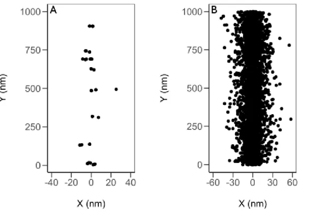
continuous dense column of energy deposition events. This is illustrated in Figure 1.2 where a proton with 150 keV energy (70 keV/µm) travels through liquid water generates a cylindrical track of densely packed energy deposition events while a proton with 300 MeV energy (0.3 keV/µm) produces a distinct “spur” track structure.
Figure 1.2: Spatial location of radiolytic species post-energy deposition from the Monte Carlo track simulation of 300 MeV protons (A) and 150 keV protons (B) (LET~ 0.4 and 70 keV/µm) incident on liquid water at 25 °C.
1.3.3 High LET radiation
As mentioned earlier, high LET radiation results in a higher frequency of energy deposition events along the track. Given a high enough density of energy deposition events along the track, spurs and other track entities will initially contact each other, leading to the formation of a cylindrical track of continuous spurs as shown in Figure 1.3. This cylindrical track has a primary “core” of energy deposition events with a surrounding region of “branches” produced via secondary electrons that emerge from the core region. (Mozumder et al., 1968; Chatterjee and Schaefer, 1976; Ferradini, 1979; Magee and Chatterjee, 1980, 1987; Mozumder, 1999; LaVerne, 2000, 2004)
12
Figure 1.3: Track structure and associated primary energy-loss events in high LET tracks. (adapted from Ferradini, 1979).
Due to the proximity of neighboring spurs in this scheme, it is more likely for species to come into contact with species produced by other spurs. An example of this would be free radicals coming into contact with other free radicals which increases the production of molecular products. In water, spurs in low LET tracks are sufficiently far apart that free radicals from different spurs are not likely to react with each other, thus increasing free radical yields. It has been observed that low LET radiation favors the yields of free radicals such as •OH, H•, and e
-aq while high LET radiation instead
promotes the production of H2 and H2O2. (Anderson and Hart, 1961; Islam et al., 2017;
Swiatla-Wojcik and Buxton, 1998)
High LET radiation can have different track structure behavior even if they have the same value for the LET. Monte Carlo simulations from our lab have been used to calculate track segments with the same LET for differing incident ions as shown in
13
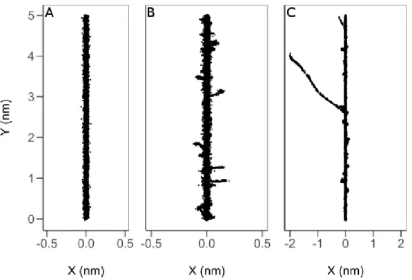
Figure 1.4: Spatial location of radiolytic species post-energy deposition from the Monte Carlo track simulation of 150 keV protons (A), 7 MeV alpha particles (B), and 306 MeV carbon ions (C) incident on
liquid water at 25 °C . Incident radiation was chosen such that the LET of the tracks would be the same
(~70 keV/µm).
Figure 1.4. We note that while all of the primary tracks can be considered similarly straight, the secondary electrons are ejected at different points with corresponding branch track distance increasing with the velocity of the primary incident ion. If we consider the total track volume to be comprised of the regions surrounding the primary core track and the surrounding the branch tracks, and that the overall energy being deposited is the same between incident ions due to their same LET, it becomes evident that the mean density of energy deposition events and subsequent reactive species decreases as the atomic number of the incident ion increases. (Muroya et al., 2006; Meesungnoen and Jay-Gerin, 2011) Variation in the radial distribution of branch tracks with different ions and the same LET is also predicted by Bethe’s theory of stopping power, (Bethe, 1930; Bethe and Ashkin, 1953) and it demonstrates that LET is not the sole determiner of the characteristics for the track structure in respect to charged
14
particles. (Schuler and Allen, 1957; Sauer et al., 1977; LaVerne and Schuler, 1987; Kaplan and Miterev, 1987; Ferradini, 1990; Ferradini and Jay-Gerin, 1999; LaVerne, 2000, 2004)
1.3.4 Track proximity: Strength in numbers?
While somewhat reductive, we can describe the passage of ionizing radiation through water as a series of energy deposition events that generate radiolytic species that then undergo interactions with the nearby water molecules or other radiolytic species. As mentioned earlier, one of the major differences between low and high LET radiation is the distance between spurs or energy deposition events which then affect whether molecular products or free radical production is promoted. We can make the argument that if multiple simultaneous (parallel) low LET tracks are in close enough proximity such that the spurs of each individual track overlap with spurs from another track, that the radiochemistry should be similar to that of a high LET track. (Kreipl et al., 2008) There should be variability in how strong of an effect this would provide depending on the distance between tracks, with maximum effect when the tracks essentially occupy the same volume and with progressively smaller effects as the distance between tracks increases. At some point this “track proximity” effect should vanish completely once the distance between tracks is large enough that the probability of a radiolytic species from one track traveling far enough to encounter a radiolytic species from another track before reacting with the surrounding water molecules drops to zero. This distance is evidently different for each radiolytic species depending on their diffusion coefficient as well as their propensity to react with the surrounding molecules, but we can assume that the effect is mostly irrelevant once the distance is more than a couple hundred nanometers.
In most practical applications, we do not expect to observe any sort of “track proximity” effect since the required conditions with generation of tracks close enough
15
in spatial proximity that their spurs overlap as well as at close enough timeframes that they develop simultaneously would involve extremely high dose rates. For example, if we assume an array of 100 parallel tracks arranged in a square grid pattern travelling for a length of 1 µm in water with each track having a LET of 1 keV/µm and that the distance between tracks is 100 nm between nearest neighbors, the amount of energy deposited in the system is 100 keV. If we assume that the irradiated volume is a simple 1 µm3 cube encompassing the tracks, this gives 100 keV deposited into 10-15 kg of
water which gives a dose of roughly 16 Gy. Even using relatively low LET tracks, we still achieve an absorbed dose in a very short time period that is significantly higher than the fractional doses used in conventional radiotherapy, with the disparity being more and more prevalent as higher LET tracks are employed or the distance between tracks is decreased.
However, in applications such as FLASH-RT, “track proximity” effects are expected since the mean dose rates involved typically range upwards of 100 Gy/s and dose rates within pulses greater than 106 Gy/s which imply that there is close proximity
between tracks. Thus in order to fully understand the mechanisms underlying high dose rate applications of radiolysis such as FLASH-RT, it is imperative that “track proximity” effects are understood.
1.4 Radiolysis of water
Radiolysis describes the interaction between ionizing radiation and molecular substances, and the subsequent chemical changes induced in the irradiated medium. In particular, the radiolysis of water involves the ionization or excitation of water molecules via interaction with ionizing radiation, which then leads to decomposition of the water molecule into a number of species depicted in Figure 1.5. The amount of any given species generated or destroyed following the radiolysis process per some unit of energy deposited into the system is known as the yield or G-value, with this work
16
defining it as “# of species per 100 eV”. This process can be divided into three different stages: the physical stage, the physico-chemical stage, and the chemical stage as depicted in Figure 1.5.(Platzman, 1958; Kuppermann, 1959)
Figure 1.5: Time scale of events in the radiolysis of pure, deaerated water using low LET radiation. (Meesungnoen, 2007; Meesungnoen and Jay-Gerin, 2010) The different colors used are for visual clarity to highlight the individual processes that occur during radiolysis.
1.4.1 Physical stage
The physical stage describes the initial deposition of energy into the water molecules which can lead to either the excitation or ionization of the water molecules which occurs within a ~10-16 s timeframe of the initial deposition event.
H2O → H2O•++ehot- (𝑖𝑜𝑛𝑖𝑧𝑎𝑡𝑖𝑜𝑛) (1.3)
H2O → H2O* (𝑒𝑥𝑐𝑖𝑡𝑎𝑡𝑖𝑜𝑛) (1.4)
Between these two processes, ionization dominates in terms of probability of occurring with it occurring ~80% of the time. The “hot” or secondary electron that is
17
released via the ionization process typically has enough energy to induce further radiolysis events in nearby water molecules which then become a key component of the physico-chemical stage. We note that the excited state denoted by H2O* is
representative of a collection of excited states which includes “super-excited” states (Platzman, 1962a), and “plasmon” type excitations (Heller et al., 1974; Kaplan and Miterev, 1987; LaVerne and Mozumder, 1993; Wilson C.D. et al., 2001).
1.4.2 Physico-chemical stage
For a short timeframe after the physical stage (up to ~1012 s after initial energy
deposition), the resulting excited/ionized water molecules decompose into various species distributed non-homogeneously in the irradiated volume. In addition, the secondary electrons produced from the ionization process may scatter away from its initial ionization event and, if it has sufficient kinetic energy, may cause further excitations or ionizations of other water molecules.
The ionized water molecules produced from reaction 1.3 may perform a proton transfer with neighboring water molecules undergoing the following reaction:
H2O + H2O•+ → H3O++ OH• (1.5)
H3O•+ (which will be referred to as Haq+) here represents the hydrated proton, while the
produced •OH molecule typically does not undergo any reactions until the chemical
stage. Another possible pathway for the ionized water molecules is via recapturing “hot” electrons undergoing thermalization through Coloumb attraction which results in the following electron-cation geminate recombination: (Meesungnoen et al., 2013; Brocklehurst, 1977)
e- + H2O•+ → H2O* (1.6)
The excited water molecules produced from reactions 1.4 and 1.6 during both the physical and physico-chemical stages undergo a de-excitation which results in a number of decomposition products. Unfortunately, there is limited information
18
available for the decay channels and associated branching ratios for excited water molecules in the liquid phase. However, the overall contribution of primary radiolysis products associated with excited water molecules is a small fraction compared to the contribution from ionized water molecules. For this reason, we assume that the de-excitation pathways are the same as that of an isolated water molecule as shown below: (Swiatla-Wojcik and Buxton, 1995; Cobut et al., 1998; Meesungnoen and Jay-Gerin, 2005a; Sanguanmith et al., 2011; Kanike et al., 2015)
H2O* → H•+ OH• (1.7)
H2O* → H2+O( D1 ) (1.8)
H2O* → 2H•+ O• •(3P) (1.9)
H2O* →H2O + thermal energy (1.10)
Here O(1D) and •O•(3P) represent the singlet 1D excited state and the triplet 3P
ground state respectively for oxygen. The branching ratios for these channels are chosen to match the observed G-values of the produced spur species at the picosecond time range. (Muroya et al., 2002; Meesungnoen and Jay-Gerin, 2005a) We note that the dissociation of the excited water molecule shown in reaction 1.7 is the primary source of the initial yield for the hydrogen atom. O(1D) atoms efficiently react with water to
form H2O2 and possibly 2 •OH. (Taube, 1957; Biedenkapp et al., 1970) However, •O•(3P) is unreactive in the aqueous phase with water but it can react with additives.
(Amichai and Treinin, 1969)
The secondary electron transfers energy as it travels through the irradiated medium via interaction with water molecules similarly to the primary ionizing radiation. However, at a certain point the secondary electron lacks sufficient energy to induce an excitation of a water molecule (~7.3 eV) which causes the secondary electron to transition to a “subexcitation” electron (esub- ) (Platzman, 1955). This subexcitation
19
vibrational and rotational modes in nearby water molecules. Over the course of ~10-40 fs (at 25 ∘C) (Goulet et al., 1990, 1996; Meesungnoen et al., 2002a), the electron is
thermalized (etherm- ) which can then become localized or “trapped” by an appropriately
sized potential well formed by nearby molecules (etrap- ). While the nature of the trapped
electron is still contentious, it quickly reaches a fully relaxed and hydrated state (eaq- )
achieved via its negative charge orienting the dipoles of the nearby molecules. For liquid water under standard conditions (25 C⃘ ), this entire process from thermalization
to hydrated state can occur within a ~240 fs to 1 ps timeframe which has been demonstrated from time-resolved femtosecond spectroscopic laser studies. (Mozumder, 1999; Meesungnoen and Jay-Gerin, 2011). Another possible pathway for an electron undergoing thermalization is via its temporary capture by a water molecule to form a transient water molecule anion which can then dissociate as follows:
etherm- +H2O →H2O•- →H- + OH• (1.11)
The produced H- anion then reacts with a neighboring water molecule as follows:
H- + H2O → H2 + OH- (1.12)
This overall process outlined in reactions 1.11 and 1.12 known as “dissociative electron attachment” or “DEA”, has been experimentally observed in amorphous solid water at ~20 K using electron energies ranging between 5 eV and 12 eV. (Rowntree et al., 1991) The production of “non-scavengeable” H2 in the early timeframe of water
radiolysis has been proposed by some groups to be primarily attributed to this DEA process, (Platzman, 1962b; Faraggi and Désalos, 1969; Goulet and Jay-Gerin, 1989; Kimmel et al., 1994; Cobut et al., 1996; Meesungnoen et al., 2015) as the yields of “non-scavengeable” H2 can be lowered via the addition of electron scavengers that
target electrons still undergoing thermalization which would compete with the DEA process. (Pastina et al., 1999) An alternative explanation has been proposed by Sterniczuk and Bartels (2016) as their recent experiments have implied that the
20
production of H2 in this early timeframe is instead dominated by the dissociation
outlined by reaction 1.8 which follows the electron-cation geminate recombination process outlined by reaction 1.6.
Following ~1ps after the initial passage of ionizing radiation, the excited and ionized water molecules have produced e
-aq, H•, H2, •OH, H2O2, H+ (or H3O+), OH-, O2
•-(or HO2•, depending on the pH), •O•(3P), etc. as radiolysis products. These various
species can then diffuse away from their original coordinates and undergo reactions with nearby water molecules or other radiolysis species. The expanding region encompassed by the diffusing initial radiolysis products is the stage for the chemical stage of radiolysis.
1.4.3 Chemical stage
The chemical stage comprises the diffusion and reactions of the radiolysis products present after the physico-chemical stage and the reestablishment of chemical equilibrium within the solution. Species present after the physico-chemical stage are initially distributed non-homogeneously with higher concentrations in “spurs” or surrounding the axis of the ionizing radiation track for low and high LET radiation respectively. These “spurs” or tracks expand during the development of the chemical stage as the species diffuse away from their initial position via macroscopic diffusion laws. The species can react with other nearby species or any solutes that have been added to the water during the diffusion process. During this process, this expansion can be divided into two substages itself, the “non-homogeneous” phase ranging from ~1ps to ~1μs after irradiation and the “homogeneous” phase which takes place ~1μs after irradiation. (Buxton et al., 1987; Sanguanmith et al., 2012) As the name implies, during the “non-homogeneous” phase the species are still relatively confined within their initial spurs or track sections with most reactions in this phase involving radicals reacting with each other to form molecular products such as H2, H2O2, and H2O, while
21
less reactive species continue to escape from their initial spurs/tracks into the bulk solution. After ~1μs, the remaining species have diffused sufficiently enough that they are now considered homogeneously distributed throughout the bulk solution thus the term “homogeneous” phase. (Plante et al., 2005; Muroya et al., 2006) At this point, reactions involving the remaining species including those produced in the “non-homogeneous” phase can be described using standard homogeneous chemistry. We note that the “non-homogeneous” phase relies heavily on the initial distribution of the spurs/track structure, thus is of particular interest when considering the development of the phase when presented with scenarios where spurs/track sections are initially placed in close proximity to each other.
1.4.4 Biological implications following radiolysis
The effects of ionizing radiation traveling through human biological systems can be roughly summed up as direct effects incurred via the ionizing radiation interacting directly with important biomolecules in the femtosecond timeframe, as well as indirect effects that occur from the generation of water radiolysis products interacting with biomolecules. While our bodies naturally incur damage from sources such as naturally occurring background radiation as well as generation of reactive species through metabolic processes, these sorts of damages are easily repaired via cellular processes. In contrast, damages caused by radiolysis tend to be clustered into very localized areas such that they challenge the natural ability of cells to repair themselves.
Direct effects typically occur within ~10-14-10-12 s from the onset of irradiation,
with the breaking of chemical bonds in biomolecules including C-H, S-H, O-H, and N-H bonds that could potentially lead to carcinogenic effects. (Sharma et al., 2011; Symons, 1994) One example of this would be direct interactions between ionizing radiation and DNA where the direct energy deposition into the DNA results in strand breaks, often multiple in close proximity, that result in future cell death. The actual
22
extent of damages attributed to the direct effect is proportional to the LET of the incident radiation, the dose rate, as well as the concentration of the species of which you wish to target with the incident radiation. Overall the efficacy of the direct effect depends on the probability that the path of the incident radiation passes through a particular molecular structure, as well as its probability of undergoing an energy deposition event while the incident radiation and molecular structure are intersecting, necessitating a high density of energy deposition events close to molecular structures.
The indirect effect takes place over a much longer timeframe than the direct effect (upwards of 10-3 s), as it involves the interactions of active species generated
from radiolysis with biomolecules. These active species include free radicals, ions, and molecular products, which are typically oxidizing. Free radicals in particular are prone to reacting to biomolecules such that the free radical undergoes a transformation with the biomolecules. This in turn causes the biomolecule in question to become a free radical itself, which causes it to potentially undergo further reactions such as electron transfers or dissociation. In any case, the free radical biomolecule or whatever products that result as it undergoes its own free radical reactions are rarely compatible with the biological system they are a part of, leading towards unfavorable biological consequences.
One example of a free radical reacting with a biomolecule is •OH reacting with
DNA nucleobases, where the lower oxidization potential associated guanine (1.29 V) leads towards other nucleobases transferring electron holes to guanine. (von Sonntag, 2006) The •OH radical may add itself to guanine to the C4-, C5-, C8-, and rarely the
C2- positions. (Dizdaroglu and Jaruga, 2011; Chatgilialoglu et al., 2009) These •
OH-adduct radicals may then undergo various reactions such as the C4- and C5- OH-adduct radicals eliminating water to form a neutral guanine radical (Gua(-H)•) (which can also
23
2’-deoxyribose in DNA which can lead to further strand breaks. (Dizdaroglu et al., 1975) Gua•+ generated from processes such as direct ionization itself may undergo
hydration to form the C8-OH-adduct radical which in the presence of oxygen undergoes oxidation to form 8-oxo-7,8-dihydroguanine (8-oxoGua) which has strong mutagenic properties. (Breen and Murphy, 1995) When oxygen is less prevalent, the C8-OH-adduct radical may undergo reversible β-fragmentation which leads towards a one-electron reduction 2,6-diamino-4-hydroxy-5-formamidopyrimidine (FapyGua) which potentially has mutagenic properties. (Dizdaroglu et al., 2008)
1.5 Research objective
The main goal of this research is to further understand of how spatial proximity of the track structures generated from ionizing radiation impact the yields of radiolytic species. With increasing focus being put on ultra-high dose rate schemes such as FLASH-RT, it becomes evident that knowing the behavior of how ionizing radiation tracks interact in close proximity will be important in understanding the mechanisms behind FLASH-RT. As it is rather difficult to consistently generate simultaneous incident ionizing particles with arbitrary separating distances on the scale needed to demonstrate a spatial proximity effect using experimental methods, we have employed Monte Carlo methods.
The SHERBROOKE Monte Carlo simulation system employed by our research group was previously incapable of modeling multiple simultaneous ionization tracks on both a technical level due to the functionality not being present, as well as a performance level as the addition of multiple ionization tracks renders most simulations computationally intractable. In this thesis we present modifications of our current SHERBROOKE system to allow for simulations involving multiple simultaneous tracks completed within a reasonable amount of time. (Chapter 2.2)