Etude des micro-contraintes dans les matériaux texturés hétérogènes par diffraction et modèles de comportement

HAL Id: pastel-00003210

https://pastel.archives-ouvertes.fr/pastel-00003210

HAL is a multi-disciplinary open access archive for the deposit and dissemination of sci-entific research documents, whether they are pub-lished or not. The documents may come from teaching and research institutions in France or

L’archive ouverte pluridisciplinaire HAL, est destinée au dépôt et à la diffusion de documents scientifiques de niveau recherche, publiés ou non, émanant des établissements d’enseignement et de recherche français ou étrangers, des laboratoires

Etude des micro-contraintes dans les matériaux texturés

hétérogènes par diffraction et modèles de comportement

Sebastian Wronski

To cite this version:

Sebastian Wronski. Etude des micro-contraintes dans les matériaux texturés hétérogènes par diffrac-tion et modèles de comportement. Sciences de l’ingénieur [physics]. Arts et Métiers ParisTech, 2007. Français. �NNT : 2007ENAM0017�. �pastel-00003210�

No : 2007-ENAM-0017

École doctorale n°432 : Science de Métiers de l’Ingénieur

THÈSE

Pour obtenir le grade de

Docteur

de

l’École Nationale Supérieure d’Arts et Métiers

et

l’Université de Sciences et Technologie AGH de Cracovie

Spécialité : Mécanique et Matériaux

Présentée et soutenue publiquement

par

Sebastian Wroński

Etude des micro-contraintes dans les matériaux texturés

hétérogènes par diffraction et modèles de comportement

Direction de thèse:

Chedly BRAHAM et Krzysztof WIERZBANOWSKI

Jury:

Andrzej KOŁODZIEJCZYK, Professeur, AGH, UST, Cracovie...…... Président

Paul LIPIŃSKI, Professeur, ENIM, Metz...…. Henryk FIGIEL, Professeur, AGH, UST, Cracovie... Jan BONARSKI, MIMI, dr hab. PAN, Cracovie...

Rapporteur Rapporteur Rapporteur Alain LODINI, Professeur, LACM, Université de Reims...

Antoni PAJA, Professeur, AGH, UST, Cracovie... Janusz WOLNY, Professeur, AGH, UST, Cracovie... Wiesława SIKORA, Professeur, AGH, UST, Cracovie...

Examinteur Examinteur Examinteur Examinteur

Laboratoire d’Ingénierie des Matériaux (LIM) ENSAM, CER de Paris Department of Condensed Matter Physics AGH, UST de Cracovie

Acknowledgements

First of all I would like to thank my supervisors: Prof. Krzysztof Wierzbanowski and Dr Chedly Braham for their guidance and help. Thanks are also due to Dr Andrzej Baczmański and Dr Jacek Tarasiuk for discussions and to all colleagues from the Group of Condensed Matter Physics (Faculty of Physics and Applied Computer Sciences, AGH-UST, Kraków, Poland) for help and friendly atmosphere.

I would like to express my thanks to Dr Wilfrid Seiler for careful planning and assistance in carrying out many experiments using X-ray diffraction and to Dr Mirosław Wróbel for preparing many samples.

I am grateful to Dr Michael Fitzpatrick for enabling my visits in the Open University, Milton Keynnes, UK. I would also like to thank Dr Ed Oliver for his help during experiment using neutron diffraction at Rutherford Appleton Laboratory, ISIS, UK.

Finally, I would like to express my gratefulness for my family and especially Justyna Wojno for her patience and support.

Résumé

Etude des micro-contraintes dans les matériaux texturés hétérogènes par

diffraction et modèles de comportement

L’objectif de ce travail est le développement d’une méthodologie d’analyse des contraintes utilisant des modèles théoriques pour décrire le comportement élasto-plastique des matériaux polycristallins. L’étude vise d’abord l’interprétation de résultats expérimentaux par des modèles de déformation qui décrivent la création des champs de contrainte dans les matériaux polycristallins déformés. Une attention particulière est portée à l’explication des phénomènes physiques à l’origine des contraintes résiduelles et à la prédiction de leur évolution et de leur influence sur les propriétés du matériau.

Dans le premier chapitre, la méthode classique, dite des sin2ψ, d’analyse des contraintes est présentée. Ensuite, la nouvelle méthode d’analyse, méthode de multi-réflexions, basée sur les mesures de déformation en utilisant plusieurs réflexions hkl est introduite. Dans cette méthode, tous les pics de diffraction sont analysés simultanément et la distance interréticulaire dhkl est remplacée par une distance équivalente a. Aussi, sont présentées les méthodes de calcul des constantes élastiques radiocristallographiques qui jouent un rôle crucial dans la détermination des contraintes. La détermination de ces constantes est indispensable pour l’interprétation des différents résultats expérimentaux. De nouvelles méthodes de calculs des constantes élastiques radiocristallographiques utilisant le modèle autocohérent ont été développées et testées. Une attention particulière a été portée au calcul par ce nouveau modèle autocohérent dans le cas des couches superficielles (surface libre). Dans ce modèle, le calcul des forces et contraintes normales à la surface est effectué selon le modèle de Reuss et pour les deux autres directions, c’est le modèle auto-cohérent qui est utilisé. Cette méthode de calcul est particulièrement adaptée au cas de la diffraction des rayons X où seulement une couche superficielle du matériau est examinée (généralement de quelques µm d’épaisseur).

Dans le chapitre suivant, deux modèles de déformation ont été développés et utilisés pour déterminer l’évolution des contraintes et analyser les propriétés du matériau. Le premier modèle (LF) est basé sur les formulations de Leffers (Lefers 1968) qui ont été reprises et développées par Wierzbanowski (Wierzbanowski 1978, 1982). Le second est le modèle auto-cohérent (SC) (Hutchinson 1964, Berveiller et Zaoui 1979). Dans ce travail, le calcul est

les grains. Les grains du polycristal sont considérés comme des inclusions ellipsoïdales (en 3D) dans une matrice homogène. Ces deux modèles de déformation elasto-plastique (LW et SC) sont des outils très utiles pour l’étude des propriétés mécaniques des matériaux polycristallins. Ils permettent la prédiction des propriétés macroscopiques du matériau (texture, courbes contrainte-déformation, surfaces d’écoulement plastique, densité des dislocations, état final des contraintes résiduelles, etc.) à partir de ses caractéristiques microsructurales (systèmes de glissement, loi d’écrouissage, texture initiale, état initial des contraintes résiduelles, etc.) (Wierzbanowski 1978). Des résultats typiques: de texture, écrouissage et énergie stockée, obtenus par ces modèles, ont été comparés aux résultats expérimentaux.

Le chapitre 3 est consacré principalement à l’explication des origines physiques des contraintes et de la prédiction de leur évolution, ainsi qu’à leur influence sur les propriétés du matériau. Les contraintes internes sont classées en trois types selon l’échelle : contraintes d’ordre I, II ou III. Une attention particulière est portée aux contraintes d’ordre I et II car ce sont les seules qui sont déterminées à partir de la position des pics de diffraction. Les modèles de déformation ont été utilisés pour l’analyse des contraintes à l’échelle des grains (contraintes du second ordre). L’évaluation quantitative de ce type de contraintes ne peut pas être effectuée directement par des mesures mais elle est possible grâce aux modèles. Les matériaux multi-phasés ont été également étudiés. Pour ces matériaux, l’interprétation des données expérimentales est plus complexe que celle du cas des matériaux monophasés en raison de la nécessité de prendre en compte l’interaction entre les phases. C’est pourquoi, une nouvelle méthode adaptée aux matériaux multi-phasés a été développée et appliquée au cas des aciers inoxydables austéno-ferritiques (aciers Duplex). Les paramètres de déformation plastique ( ph

c

τ - scission critique résolu et ph

Η - paramètre d’écrouissage) de chacune des phases ont pu être déterminés. Lors de la déformation plastique, l’évolution des contraintes dans les phases et la création de contraintes d’incompatibilité de second ordre, sont observées et l’influence de la texture cristallographique et de l’anisotropie élastique est étudiée. La méthodologie développée et utilisée dans ce travail a, donc, permis de déterminer quantitativement les contraintes du premier et du second ordre, pour chaque phase. Il a été montré qu’une bonne corrélation entre les déformations déterminées expérimentalement et les résultats théoriques, n’est obtenue que si l’influence des contraintes du second ordre est prise en compte. Aussi, le meilleur lissage des courbes expérimentales est obtenu quand les calculs intègrent les constantes d’élasticité anisotropiques et la texture réelle initiale de

Les méthodes de détermination des contraintes du premier et du second ordre, présentées au troisième chapitre, sont employées pour l’étude des contraintes résiduelles dans des alliages écrouis par laminage croisé (Chapitre 4). Le laminage croisé a été retenu pour ajouter une symétrie de la texture cristallographique et, donc, de réduire l’anisotropie de la pièce (comparé au laminage uniaxial). Les résultats sont présentés pour des séries d’éprouvettes en acier et en alliage de cuivre. Dans le cas de l’alliage de cuivre, les résultats montrent de très faibles niveaux de contraintes d’incompatibilité de second ordre qui peuvent être négligées. Par contre, dans le cas de la ferrite, il faut en tenir compte car leur niveau s’avère important. Les oscillations observées sur les courbes des sin2ψ peuvent être expliquées, dans ce cas, principalement par la présence de contraintes du second ordre.

Enfin, au chapitre 5, une nouvelle méthode d’analyse des contraintes utilisant un faisceau de rayons X avec un angle d’incidence faible et constant (méthode de diffraction en incidence rasante GID-sin2ψ). Cette méthode présente l’avantage d’une profondeur de pénétration des rayons X constante, contrairement à la méthode des sin2ψ classique qui présente l’inconvénient d’une forte variation de la pénétration avec l’angle ψ. C’est pour cette raison que la méthode classique des sin2ψ est mal adaptée pour l’étude des matériaux à forts gradients de contraintes. Moyennant un choix optimisé des angles d’incidence et du type de rayonnement, la nouvelle méthode s’avère efficace pour l’étude des matériaux à forts gradients de contraintes, en permettant des mesures dans différentes couches proches de la surface. L’incertitude des mesures a été évaluée et le rôle de l’absorption, de l’indice de réfraction et des facteurs de Lorentz-polarisation et de diffusion atomique ont été étudiés. A partir de mesures sur des poudres de référence, l’influence de chacun de ces paramètres a été évaluée et prise en compte dans la détermination de la position des pics de diffraction. Les analyses effectuées ont confirmé la faible influence de l’absorption et des facteurs de Lorentz-polarisation et de diffusion atomique sur la contrainte déterminée. Par contre, ils ont révélé un effet important de l’indice de réfraction, en particulier aux petits angles d’incidence. Pour des angles d’incidence α≤100, les corrections sont importantes et modifient les résultats des contraintes d’une manière significative (la correction peut atteindre 70 MPa dans le cas de la poudre). Cet effet et, donc, la correction nécessaire décroît quand l’angle d’incidence augmente.

Table of Contents

Summary... 3

Chapter 1 ... 5

Determining of stresses in polycrystalline materials... 5

1.1. Introduction ... 5

1.2. Measurements of macrostresses using diffraction method... 6

1.3. Diffraction elastic constants ... 13

1.4. Calculation of diffraction elastic constants ... 15

1.4.1. Diffraction elastic constants for quasi-isotropic material... 15

1.4.2. Diffraction elastic constants for anisotropic material (textured) ... 18

1.5. Multi-reflection method for stress determination... 25

Chapter 2 ... 27

Deformation models for polycrystalline materials ... 27

2.1. Introduction ... 27

2.2. Mechanisms of plastic deformation... 28

2.3. Macroscopic description... 29

2.4. Behaviour of a grain ... 31

2.4.1. Slip system... 31

2.4.2. Hardening of slip systems ... 32

2.4.3. Grain deformation and lattice rotation... 34

2.4.4. Mascroscopic deformation ... 35

2.5. Leffers-Wierzbanowski plastic deformation model (LW) ... 35

2.6. Self-consistent model (SC)... 39

Chapter 3 ... 57

Residual stresses and elastoplastic behaviour of stainless duplex steel... 57

3.1. Introduction ... 57

3.2. Classification of stresses ... 58

3.3. Origin of stresses... 60

3.4. Measurements of macrostresses using diffraction ... 63

3.5. Multiphase materials ... 65

3.6. Calculation of the second order incompatibility stresses... 67

3.7. Analysis of incompatibility stresses in single phase materials ... 68

3.8. Analysis of incompatibility stresses in multiphase materials ... 81

3.8.1. Material and experimental method ... 81

3.8.2. Modelling and experimental data... 83

3.9. Conclusions ... 98

Chapter 4 ... 101

Variation of residual stresses during cross-rolling...101

4.1. Introduction ... 101

4.2. Residual stresses and texture in cross-rolled polycrystalline metals ... 101

4.2.1 Copper ... 101

4.2.2. Low carbon steel ... 109

4.3. Conclusions ... 117

Chapter 5 ... 119

Grazing angle incidence X-ray diffraction geometry used for stress

determination...119

5.1. Introduction ... 119

5.2. Classical and grazing incidence diffraction geometry for stress determination .... 120

5.3. Corrections in grazing incidence diffraction geometry... 125

5.3.1 Absorption Factor ... 126 5.3.2 Lorentz-Polarization Factor ... 128 5.3.3. Structure factor... 129 5.3.4. Refraction factor ... 130 5.4. Experimental results... 133 5.5. Conclusions ... 144

General conclusions ... 145

Lorentz-Polarization Factor ... 147

List of author’s publication ... 152

Participation in conferences ... 153

Summary

The aim of this work is to develop the methodology of stress measurement using theoretical models describing elasto-plastic behaviour of polycrystalline materials. The main purpose is to interpret experimental results on the basis of the self-consistent model which describes the mechanisms of stress field generation in deformed polycrystalline materials. Special attention has been paid to the explanation of the physical origins of stresses and to the prediction of their evolution and influence on material properties.

In Chapter 1 the classical method of stress measurement called sin2ψ was described. The new stress analysis – multi-reflection method - based on strain measurements using a few reflections hkl is introduced (in this method all peaks are analysed simultaneously). Also the methods of calculation of the diffraction elastic constants, which play a crucial role in the stress analysis, were presented. The determination of these constants is essential in explanation of many experimental results. New methods for the calculation of diffraction elastic constants using the self-consistent model have been elaborated and tested. These methods were used for textured samples.

In Chapter 2 two models (self-consistent and Leffers-Wierzbanowski models) were presented. They enable the prediction of macroscopic material properties (e.g., texture, stress-strain curves, plastic flow surfaces, dislocation density, final state of residual stress, etc.) basing on the micro-structural characteristics (crystallography of slip systems, hardening law, initial texture, initial residual stress state, etc.).

In Chapter 3 a special attention has been paid to the explanation of physical origins of the stresses and to the prediction of the stress evolution and their influence on material properties. The internal stresses were divided into three types in function of the scale. The deformation models were used to analyse the stresses present in grains (the second order stresses). Quantitave estimation of this kind of stresses is possible only by means of models; they cannot be measured directly. Interpretation of experimental data for multiphase material is more complex than for a single phase one, because it is necessary to consider interaction between phases. For this reason, the new method of investigation of multiphase materials was developed and applied for duplex stainless steel.

The methods of estimation of the first and the second order stresses which were presented in the third chapter are used to study the residual stresses in materials after cross rolling (Chapter 4). The cross-rolling is applied in order to symmetrize the crystallographic texture and consequently, to decrease the sample anisotropy. The results for series of copper and steel samples are presented.

Finally, in Chapter 5 a new method of stress estimation using a constant and low incident beam angle (grazing angle incidence X-ray diffraction technique) was presented. In this method, the penetration depth is almost constant on the contrary to classical method. For this reason, the grazing incidence diffraction technique can be used to investigate materials with a significant stress gradient. Measurement uncertainties in this method were considered; especially the influence of absorption, Lorentz-polarization, atomic scattering factor and refractive index were studied.

Chapter 1

Determining of stresses in polycrystalline

materials

1.1. Introduction

The internal stresses are generated by applying external loads to the sample. They appear after deformation of the material as a result of a change of the shape and volume. In most cases the stress field is homogeneous and anisotropic. During plastic deformation the sample is deformed irreversibly and stresses remain in the sample even if external forces are unloaded. The stresses which can be found in unloaded samples are called the residual stresses. Residual stresses affect the mechanical properties of materials and they are responsible for such processes like fracture, cracks growth, fatigue, creep, recrystallisation and many others. However in some cases the residual stresses improve selected properties of materials. For example the presence of the compression stress field can improve endurance for cracking.

There are several techniques for determination of residual stresses, such as the destructive mechanical methods (layers removal), the methods based on the measurements of material properties affected by stresses (ultrasonic methods, measurement of Barkhausen magnetic noise, Raman spectroscopy) and the diffraction method based on the measurement of strain of the crystallographic lattice. The advantage of the diffraction method is its non-destructive character and the possibility of macro and microstress analysis in multiphase and anisotropic materials. This method is frequently used in industry, material science, electronics and biomaterial technology. Because of high absorption of X-ray radiation this method can be applied to study residual stresses to the depth of few µm below the surface of sample. In order to get deeper penetration, synchrotron or neutron radiation has to be applied. The use of synchrotron or neutron radiation enables to study stresses up to a few cm below the surface and sometimes in the entire sample volume.

In the case of synchrotron or neutron radiation the sampling volume can be well defined by special slits forming the incidence and the diffracted beams. In this way the measurement

from small selected parts of the sample can be done. The stress measurement is possible with high spatial resolution (less than 20µm). In this work, the classical X-ray and the neutron diffraction methods are used to study the stress fields in polycrystalline materials. The influence of various types of stress on the results of a diffraction experiment is discussed.

1.2. Measurements of macrostresses using diffraction

method.

When internal stresses are present in a material a systematic change of the lattice parameter in each grain is observed. The interplanar spacing is described by Bragg’s law:

λ

θ n

d_hkl sin =

2 _{{ }} (1.1)

The increase of interplanar spacing d{hkl} causes a decrease of θ angle. In typical cases the shift of

a peak is: 0,0010 - 0,10. It seems to be a small value, however a good fitting procedure of the diffraction peak (using Gauss or Lorentz function) enables to observe and measure this effect. The presence of internal stresses causes not only a shift of a diffraction peak ( ∆(2θ)= 2θ - 2θ0 ) but also a change of its intensity and width (this latter is expressed as FWHM, i.e., full width at half maximum).

a. b.

Fig. 1.1. Diffraction on a stress free lattice (a) and on a deformed lattice (b). A range of

interplanar spacings in different diffracting crystallites is shown by dashed lines, while the continuous line is used to mark the average distance between reflecting planes.

The lattice parameter can be determined using diffraction method. The measured value is the average over the group of diffracting grains. This kind of average will be marked as <...>. Hence, the Bragg law can be written as:

λ

θ n

dhkl > < hkl >= < { } sin { }

An important condition concerning the sensitivity of the method can be derived from Bragg law. A small change of interplanar spacing (∆<d >_{hkl}) is related with a shift of the peak position (∆<2θ >_{hkl}) by equation: } { } { } { } { } { } { 2 2 2 _{hkl hkl hkl} hkl hkl hkl tg tg d d > < > < − = > <         > < > < ∆ − = > < ∆ θ θ ε θ (1.3) where: } { } { } { hkl hkl hkl d d > < > < ∆ = > <ε

It is visible that for the same value of

} { } { hkl hkl d d > < ∆

, bigger shift of∆<2θ >_{hkl} is observed for higher 2θ scattering angle. For this reason usually the peaks with 2θ angle higher than 900 are used for the stress measurement. In the case of diffraction peaks with 2θ smaller than 900 the precision of measurement is generally not good enough (let us remark that the detector position is usually set with the precision of 0,010). This is why the measurements for angles smaller than 900 are not reliable (Bojarski, 1995)

2θ_{hkl} [ o ] 40 60 80 100 120 140 160 180 ∆ 2 θ{hk l} [ o ] 0.00 0.02 0.04 0.06 0.08 ∆d_{hkl}/d_{hkl} = 0.001 Fig. 1.2. ∆2θ{hkl} vs. 2θ{hkl} for 0.001 } { } { = ∆ hkl hkl d d

. It should be noticed that shift of the peak 211 for steel under pressure 200MPa equals 0,10 .

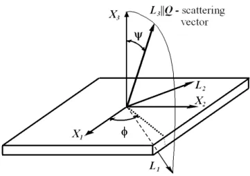
Let us describe now the measurement geometry. The experiment consists of the sample rotation around the scattering vector Q for a fixed 2θ angle. Two types of the coordinate system should be considered: sample system (X) and the measurement coordinate system (L). The definition of these coordinate systems is presented in Fig. 1.3. L3 axis is parallel to the scattering vector Q. During the measurement a sample is rotated and the position of the vector L3Q is

Fig. 1.3. Orientation of the scattering vector with respect to the sample system X. The ψ and

φ angles define the orientation of the L system ( L2 axis lies in the plane of the sample surface). The laboratory system, L, defines the measurement of the interplanar spacings <d(ψ,φ)>{hkl} along the L3 axis.

Fig. 1.4. Eulerian cradle used to change the relative sample orientation.

Bragg’s law enables to measure interplanar spacing d=d{hkl}. So for each orientation of vector L3Q it is possible to measure interplanar spacing d(ψ,φ){hkl} for crystallographic planes {hkl} perpendicular to the scattering vector Q. In all relations expressed in L coordinate system the index (‘) will be used (e.g., the measured deformation along L3 axis is marked as ε33'). The diffraction method enables to measure the mean interplanar spacing <d(ψ, φ)>{hkl}, averaged over reflecting crystallites. The mean lattice strain <ε(ψ, φ)>{hkl} in L3 direction (Fig. 1.3) is defined as:

} { 0 } { 0 } { } { 33 ) , ( ) , ( ' hkl hkl hkl hkl d d d > − < = > <ε ψ φ ψ φ _(1.4)

The lattice strain ε₃₃'(ψ,φ){hkl} for a given grain can be calculated from Hook’s law: ' ) , ( ' ) , ( ' { } 33 33 ψ φ hkl s ij ψ φ σij ε = (1.5)

where ε'_ij, σ'_mn and s'_ijmn are the elastic strain, stress and elastic compliance tensor of a grain. In the above equation the convention of repeated index summation is applied (Einstein convention). This convention will be used in the whole present work and it will concern always lower indices. For a given orientation of the scattering vector (Q) and for a given Bragg’s angle (2θ) only those crystallites diffract which have one of the {hkl} planes perpendicular to QL3 . This group of

crystallites is called diffracting group. Average measured deformation is:

> =<

>

<ε₃₃'(ψ,φ) _{hkl} s_33ij'(ψ,φ)σ_ij' (1.6)

It is next assumed that an effective tensor Sijkl’ exists for the diffracting group which simplifies the above relation to:

' ) , ( ' ) , ( ' _{{ } 33} 33 M ij ij hkl S ψ φ σ φ ψ ε > = < (1.7)

where σMij is the average macroscopic stress, constant in a big part of a sample (i.e., in the measurement volume).

Let us note that even if a sample has the quasi-isotropic symmetry (random texture), the diffracting group has a lower symmetry. Orientation of the crystallites belonging to this group can differ one from another by rotation γ around QL3Nhkl vector – Fig. 1.5. Consequently,

the average elastic matrix Smn for diffracting group has the same structure as a body with axial symmetry. It is defined by five independent parameters and has a form (see e.g., Reid, 1974):

                  = 66 44 44 33 13 13 13 11 12 13 12 11 mn ' S ' S ' S 0 0 ' S ' S ' S ' S ' S ' S ' S ' S ' S ' S _(1.8)

In the above equation the matrix notation (Smn) was used for tensor components (Sijkl). The rules for the reduction of indices are following:

Tensor indices Reduced matrix indices 11 → 1 22 → 2 33 → 3 23, 32 → 4 13, 31 → 5 12, 21 → 6 (1.9)

e.g., the tensor component S1123 becomes the matrix component S14. In the present work the elastic constant tensors will be used both in matrix and tensor convention, depending on the case in order to simplify equations.

It is evident, that the symmetry axis for the assembly of diffracting grains is QL3.

Using the elastic constants matrix, equation 1.7 can be written as: ' ' ' ' ' ' ) , ( ' _{31 11 32 22 33 33} 33 M M M hkl S σ S σ S σ φ ψ ε > = + + < (1.10)

On the right hand there are only three components, because S’34=S’35=S’36= 0 (see. Eq. 1.8).

Fig. 1.5. Definition of lattice rotation around the scattering vector L3=N{hkl} Q

Taking into account the structure of the S’mn matrix (Eq. 1.8), the above equation can be rewritten as: ' ' ' ' ' ' ) , ( ' { } 13 11 13 22 33 33 33 M M M hkl S σ S σ S σ φ ψ ε > = + + < (1.11)

Let us note that all quantities in the above equation are expressed in L coordinate system. Our goal is to relate the measured deformation ε33’ (expressed in L coordinate system) in function of stress components σij (expressed in X coordinate system). To transform stress tensor σij to L coordinate system, the transformation matrix has to be defined. This matrix is (see Fig.1.3):

          − − = ψ ψ φ ψ φ φ φ ψ ψ φ ψ φ cos sin sin sin cos 0 cos sin sin cos sin cos cos ij a (1.12)

The transformation law for four stress rank tensors is:

kl jl ik ij a a σ

σ '= (1.13)

According to the above, three needed components σii’ are:

M M M M M M M M M M M M M M M M M M 23 13 12 2 33 2 2 2 22 2 2 11 33 12 2 22 2 11 22 23 13 12 2 33 2 2 2 22 2 2 11 11 2 sin sin 2 sin cos sin 2 sin cos sin sin sin cos ' sin cos 2 cos sin ' 2 sin sin 2 sin cos cos 2 sin sin cos sin cos cos ' ψσ φ ψσ φ ψσ φ ψσ ψ φ σ ψ φ σ σ ψσ φ φ σ φ σ σ ψσ φ ψσ φ ψσ φ ψσ ψ φ σ ψ φ σ σ + + + + + = − + = − − + + + = (1.14)

After substituting the stress components from Eq. 1.14 to Eq. 1.11 we obtain:

ψ φ σ φ σ σ σ σ ψ σ ψ φ σ φ σ φ σ φ ψ ε 2 sin ) sin cos ( 2 1 ) ( cos 2 1 sin ) sin 2 sin cos ( 2 1 ) , ( ' 23 13 2 33 22 11 1 2 33 2 2 2 22 12 2 11 2 } { 33 + + + + + + + + + + = > < M M M M M hkl s s s s (1.15) where: 31 1 31 33 2 (S' S' ), s S' s 2 1 _{= − =} (1.16)

The quantities s1 and ½ s2 are so called diffraction elastic constants for a quasi-isotropic material. Eq. 1.15 can be also expressed by interplanar spacings d{hkl} (see Eq. 1.4):

} { 0 } { 0 23 13 2 33 22 11 1 2 33 2 2 2 22 12 2 11 2 } { 2 sin ) sin cos ( 2 1 ) ( cos 2 1 sin ) sin 2 sin cos ( 2 1 ) , ( hkl hkl M M M M M M M M M hkl d d s s s s d +    + + + + + + + + +   = > < ψ φ σ φ σ σ σ σ ψ σ ψ φ σ φ σ φ σ φ ψ (1.17)

Using obvious trigonometric identities the above equation can be converted to:

(

)

(

)

[

]

[

]

[

(

)

]

ψ

φ

σ

φ

σ

σ

φ

φ

φ

φ

ψ

An important simplification is obtained if one assumes a particular plane state of stress, which occurs usually on the surface of rolled samples. In such the case:

0 , 0 , 0 22 33 12 13 23 11 ≠ ≠ = = = = M M M M M M σ σ σ σ σ σ (1.19)

The rolled samples have orthorhombic symmetry and for this reason only the main stress components - σiiM -occur (symmetry axes are determined by the edges of the sample). Moreover, the static equilibrium condition on the surface involves: σ33M=0. During X-ray diffraction measurement only a thin layer of a material near the surface is examined. (see for example: Noyan and Cohen, 1987; Dolle, 1979; Hauk, 1986; Brakman, 1987, Major et al., 1999; Bochnowski et al., 2003) Consequently, the approximation of the plane state of stress is correct in such the case. However, the assumption of σ33M=0 can not valid in the case of the neutron diffraction technique, because due to very low absorption the neutron beam penetrates up to several centimetres inside the sample. (Allen et al. 1981; Daymond and Priesmeyer, 2002; Fitzpatrick and Lodini, 2003)

Assuming the approach of plane state of stress, Eq. 1.18 takes the form:

} { 0 } { 0 22 11 1 2 2 22 2 11 2 }

{

(

cos

sin

)

sin

(

)

2

1

)

,

(

s

s

d

d

d

>

=

_



+

+

+

_



+

<

ψ

φ

σ

φ

σ

φ

ψ

σ

σ

We can conclude that in the case of a quasi-isotropic sample and plane stress state the linear relation of <d(ψ,φ)>{hkl} versus sin2ψ occurs (for a fixed φ value) - Fig. 1.6.

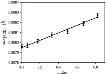
sin2Ψ 0.0 0.2 0.4 0.6 0.8 < d >{4 2 0 } [A ] 0.8078 0.8079 0.8080 0.8081 0.8082 0.8083 0.8084

Fig. 1.6. The lattice parameter <d>{420} in function of sin2ψ for copper. The slope of the curve equals ½ s2σ11M when ϕ=0.

Information about stress components is contained in the slope of the curve (Eq. 1.20). For example, if φ=00 we can determine the value of σ11Mcomponent from the slope of the diagram. Similarly, if φ=900, it is possible to determine the stress components σ22M. Generally, to obtain a good precision of determined stress components σ11M and σ22M, the experiment is repeated for different ϕ angles and the least squares procedure is applied.

In the case of neutron or synchrotron diffraction Eq. 1.18. cannot be simplified. The both techniques give the information from the whole sample volume and the assumption σ₃₃M =0

is no more valid. In general the value of d_{hkl0 _} is unknown, hence for orthorhombic and quasi-isotropic sample the values of ( 11 33 )

M M σ σ − and ( 11 22 ) M M σ σ − instead of σ11Mand M 22 σ are determined.

1.3. Diffraction elastic constants

The important step in residual stress measurement is the determination of so called diffraction elastic constants. A general definition of diffraction elastic constants is obtained from Eq. 1.7: ' ) , ( ' ) , ( ' _{{ }} 33 M ij M ij hkl R ψ φ σ φ ψ ε > = < (1.21) with : ' ' 33ij M ij S R = (1.22)

RijM’ are macroscopic diffraction elastic constants and σijM’ is the macro-stress, i.e., the average stress in a big macroscopic part of a material. They depend not only on ψ and φ angles but also on diffracting plane {hkl}. These constants are essential for interpretation of the results of residual stress measurement. The diffraction elastic constants can be calculated (Baczmański et al., 1993) and also determined experimentally.

Combining Eq. 1.6: <ε₃₃'(ψ,φ)>_{hkl}=<s_33ij'(ψ,φ)σ_ij'> and Eq. 1.21 we can write: > =< '( , ) ' ' ) , ( ' 33ij ij M ij M ij s R ψ φ σ ψ φ σ (1.23)

In general R’ij(ψ,φ) cannot be calculated in a direct way, because elastic interactions between grains in polycrystalline sample are quite compliex. For these reason we use some simplifying assumptions or models. Eq. 1.18 can be rewritten in terms of R33M’ and R11M’ (using Eqs. 1.16 and 1.22) as:

(

)

[

(

)

(

)

]

{

[

] (

) (

)

[

(

)

]

}

ψ

σ

φ

σ

σ

φ

φ

φ

φ

ψ

In general, the aim of experiment is to find residual stresses expressed in X coordinates system (σij). Hence, it is convenient to establish the relation between (<ε33'(ψ,φ)>{hkl}) and σij (while Eq. 1.21 contain stresses in L coordinate system). This aim is achieved by introducing modified elastic diffraction constants Fij and instead of Eq. 1.21 we have:

M ij M ij M ij hkl F R ψ φ σ φ ψ ε₃₃'( , )>_{{ }}= ( , , ) < (1.25)

whereσijM are the macrostresses expressed in X coordinate system. The

M ij

F coefficients are not

tensor components because they relate the stress tensor σijMexpressed in the sample coordinate

system X to the elastic strain < ε'₃₃g(el)>{hkl} defined along L3 axis of the L system. Using the

appropriate transformation of stress tensor (Eq. 1.13), the F diffraction elastic constants can be ijM

calculated from Rij ones:

) , }, ({ ) , }, ({hkl ψ φ a a R hkl ψ φ F M kl lj ki M ij = (1.26) For example: ψ φ ψ φ ψ φ ψ φ φ ψ φ sin sin sin cos cos sin sin cos sin cos cos 23 13 12 33 22 11 11 2 R 2 R + 2 R R + R + R = F M 2 M M 2 2 M 2 M 2 2 M M − − (1.27)

It should be emphasised that the RijM constants, as noted in Eq. 1.21, depend on the

orientation of L system with respect to X one if the sample is textured. However, in the case of a polycrystalline with random grain orientations (quasi-isotropic sample), the R'ij constants do not

1.4. Calculation of diffraction elastic constants

As it was already mentioned, diffraction elastic constants are the main parameters used in the analysis of residual stresses by diffraction method. In general it is not possible to find equation expressing R’ij(ψ,φ) due to a complex character of elastic interactions. For this reason some simplifying assumptions and models are used.

1.4.1. Diffraction elastic constants for quasi-isotropic

material

The quasi-isotropic polycrystalline material is defined as a material having isotropic macroscopic properties in spite of the anisotropy of particular grains (Bunge, 1982). For a quasi-isotopic material the following relation occurs:

R R R23M 0 M 13 M 12 = = = and M M R R11 = 22 (1.28)

Consequently, only two independent diffraction elastic constants, i.e.: R₁₁M =R₂₂M and R33M exist.

These diffraction elastic constants are defined with respect to the L coordinates system and they do not depend on its orientation characterized by the angles φ and ψ (Fig.1. 3).

For quasi-isotropic materials the s1 and s2 diffraction elastic constants are commonly used instead

of the more general R constants. In this case the following relations are fulfilled (compare Eq. ijM

1.16): M 22 M 11 1 R R s = = and ( 11M) M 33 2 R R s 2 1 _{= −} (1.29)

Hence, the exemplary equation for F11 constant (Eq. 1.27) for quasi-isotropic material can be

simplified to: s 2 1 + s = F 1 2 2 2 M ψ φsin cos 11 (1.30)

The s1 and s2 constants can be also expressed by the Young's modulus (E') and Poisson's ratio

( 'ν ) defined for a group of diffracting grains, interacting with the surrounding matrix (E' and 'ν are expressed in L system, i.e., for example the Young's modulus is taken along L3axis). The s1

and s2 constants are equal to:

E = s1 ′ ν′ − and E + 1 2 = s2       ′ ′ ν _(1.31) where: R 1 = E _M 33 ′ and _M 33 M 22 M 33 M 11 R R = R R =− − ′ ν .

We can conclude that for a quasi-isotropic polycrystalline material only two independent diffraction elastic constants are defined (i.e., s1 and s2 or 22M

M 11 R

R = and R33M ) with respect to L

system. These elastic constants depend on the single crystal constants, grain-matrix interaction and hkl reflection, but they do not depend on φ and ψ angles. A linear relation of F versus 11M sin2ψ (for a fixed φ value) can be easily seen from Eq. 1.30.

In further considerations the effects of crystal anisotropy (existing also in a quasi-isotropic sample) will be characterized by the factor Γ{hkl} (Dölle, 1979).:

(

)

(

)

The Γ{hkl} factor depends only on Miller indices of reflecting planes and it varies in the range (0,1/3). It has the minimum and the maximum for {100} and {111} crystal planes, respectively. We will calculate now the diffraction elastic constants for a quasi-isotropic material using two limiting models of elasticity.

Voigt model

In this approach (Voigt, 1928) the constant elastic deformation in each grain “g” is assumed:ε'_ijg(el)=ε'_ijM(el) (Fig 1.9). It means that

< >hkl = M33el =[c g ]_33ij1 _ijM el g 33 ' ' ' { } ( ) ) ( ε σ ε _′ − _(1.33) R =[c ]33ij g V M ij 1 ) ( ′ − _(1.34)

where […] means the average over the volume sample.

Diffraction elastic constants s1V and ½ s2V for quasti-isotropic material with regular lattice are (Noyan and Cohen, 1987):

(

)

(

)

(

)

(

)

(

)

(

)

Diffraction elastic constants in this model do not depend on reflecting plane indices {hkl} and on the Γhkl factor.

Reuss model

In this case a constant stress is assumed in all grains: ijM er

g

ij '

' ( ) σ

σ = (Fig. 1.8); the superscript

“er” means: “elastic reaction” (of a grain). Elastic constants for the group of diffracting grains can be expressed by single crystal compliance constants (Noyan and Cohen, 1987):

{ } '

(

(

)

)

(

)

(

)

After substitution of the above equation to Eq.1.31, anisotropic elastic constants are: s₁R_,{hkl}=S₁₂ +

(

)

(

)

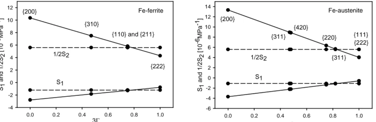
In this case diffraction constants depend on the refelecting plane {hkl}. Diffraction elastic constants for Reuss and Voigt models for ferrite and austenic steel are presented in Fig 1.7. They were calculated using stiffness elastic tensor presented in Table 1.1. The compliance tensor presented in equations is an inverse of the stiffness tensor.

Table 1.1. Single crystal elastic constants used for the calculation of diffraction elastic constants

(Simoms and Wang, 1971; Ceretti, 1993).

Material C11 [GPa] C12 [GPa] C44 [GPa] Fe-austenite 197 122 124 Fe-ferrite 231 134.4 116.4 TiN 497 105 168 Cu 170 124 64.5 Al 106.8 60.4 28.3 SiC 350 140.4 233

3Γ 0.0 0.2 0.4 0.6 0.8 1.0 S1 a n d 1 /2 S2 [ 1 0 -6M P a -1] -4 -2 0 2 4 6 8 10 12 S1 1/2S2 {200} {310} {110} and {211} {222} Fe-ferrite 3Γ 0.0 0.2 0.4 0.6 0.8 1.0 S1 a n d 1 /2 S2 [ 1 0 -6M P a -1] -6 -4 -2 0 2 4 6 8 10 12 14 S1 1/2S2 {200} {311} {220} {111} {420} {311} {222} Fe-austenite

Fig. 1.7. The s1 and ½ s2 constants versus orientation factor 3Γ calculated from the single crystal data using Reuss (solid line) and Voigt (dotted line) models.

1.4.2. Diffraction elastic constants for anisotropic material

(textured)

In many cases we cannot assume isotropic interaction between grains, then we talk about anisotropic material. Anisotropic interaction is a result of texture, anisotropic properties of the grains and shapes of the grains. Because of sample anisotropy, the six independent elastic constants R vary with orientation of the scattering vector. The values of ijM

M ij

F must be known

for each orientation of the scattering vector for which the interplanar spacings are measured. The anisotropy of the sample can be observed as nonlinearities of the F versus sin11M

2ψ

plot. To

calculate diffraction elastic constants we have to use appropriate model of interactions between grains. We will consider the following models:

Reuss model

In this approach the stress is assumed to be uniform across the sample (Barral et al., 1987; Brakman, 1987; Reuss, 1929) for all polycrystalline grains, i.e., σ'_ijg(er) = σ'_ijM (Fig. 1.8). The grain elastic strain in the L3 direction (Fig.1.3) can be written as:

M ij g ij 33 er g ij g ij 33 el g 33 = s' ' s' ' ' ( ) σ ( ) σ ε = and < _> =< s _>hkl M_ij g ij 33 hkl el g 33 ' ' ' { } { } ) ( σ ε (1.38)

where s'33gij are the single crystal compliances of a grain and all quantities are expressed in L

Fig. 1.8. Scheme of interaction between grains for Reuss model - homogeneous stress.

Consequently, using the Reuss model, the diffraction elastic constants can be calculated as the average value of single crystal compliances:

)d f( )d f( ) ( s = > s < = R l k h l k h 2 0 l k h l k h g ij 2 0 hkl g ij R M ij ) ( } { ) ( } { 33 } { 33 ) ( ' '

∑ ∫

∑ ∫

The integration is carried over all g orientations representing reflecting grains only (these orientations are inter-related by the rotation γ _{around the scattering vector, see Fig. 1.5.} Moreover, the averaging over all equivalent {hkl} planes is done.

Voigt model

The uniform grain elastic strain is assumed to be equal to the elastic macro-strain value ) ( ) ( ' ' Mij el el g ij ε

ε = in the Voigt model (Voigt 1928) - Fig. 1.9.

Fig. 1.9. Scheme of interaction between grains for Voigt model - homogeneous strain. In this case the grain elastic strain in the L3 direction can be written as:

' ] c [ = ' = ' > ' < {hkl} M33(el) g _33ij1 M_ij ) el ( g 33 } hkl { ) el ( g 33 =ε ε ′ σ ε − _(1.40)

where c is the single crystal stiffness tensor defined with respect to L'g frame. The average, marked by […], is calculated over the whole considered volume. Finally, the RijM(V) constants are

] c [ = R 33ij g V M ij 1 ) ( ′ − _(1.41)

The texture function f(g) is again used in the calculation of RijM(V) constants; however in this

model all grains from the studied volume contribute to the average:

g g g f( )d c 8 1 = ] [c g ijkl E 2 g ijkl ' ( ) '

∫

In the above equation the single crystal stiffnesses c'_ijklg (g) (considered in L system) is integrated over the whole orientation Euler space (E). Because the integration is over the whole Euler space the elastic constants do not depend on {hkl} plane.

Self-consistent model

In the self-consistent model (Baczmański et al., 1997b and 2003c; Kröner 1961; Lipiński and Berveiller 1989) a polycrystalline grain is considered as an ellipsoidal inclusion inside a homogeneous continuous medium (Fig. 1.10).

Fig. 1.10. Scheme of interaction between grains for self-consistent model. Ellipsoidal inclusion

is embedded in a homogeneous medium.

According to this formalism, the elastic strain ε'_nmg(el) (or stress σ'g_nm(er)), in the g-th grain,

is related to the macrostrain 'ε M_kl(el)(or macrostress σ'M_kl ) by the concentration tensorA'g(sc) (or ) ( 'g sc B ), i.e.: A M el kl sc g mnkl el g nm ' ' ' ( ) ( ) ( ) ε ε = and σ'_nmg(er) =B'g_mnkl(sc)σ'_klM (1.43)

where A'g(sc) and B'g(sc)=c'g A'g(sc)S'eff are the strain and stress concentration tensors calculated for a purely elastic interaction using the self-consistent method, S'eff is the macroscopic compliance tensor (S'eff will be described in Chapter 2) and c is the grain 'g stiffness tensor expressed in L system.

Substituting the Hook's law in macro and micro scales ( klM

eff ijkl el M ij = S' ' ' ( ) σ ε and ' ( ) 'ijkl 'gkl(er) el g ij =s σ ε )

X Mkl sc g kl 33 el g nm ' ' ' ( ) ( )σ ε = (1.44) where: X'₃₃g(sc_kl)=A'g₃₃(sc_mn) S'eff_mnkl or X'₃₃g(_klsc)=s'g_33mnB'_mnklg(sc).

Finally, the diffraction elastic constants Rij(sc)for a textured sample are defined as:

)d f( )d f( ) ( X = > X < = R l k h l k h 2 0 l k h l k h sc g ij 2 0 hkl sc g ij sc M ij ) ( } { ) ( } { ) ( 33 } { ) ( 33 ) ( ' '

∑ ∫

∑ ∫

where the integration is carried over all g orientations representing reflecting grains.

For the calculation of the X'g(sc) tensor, the macro-compliance tensor S'eff for a polycrystalline aggregate must be known. To do this, the self-consistent algorithm is applied for the elastic range of deformation. For textured material the macroscopic stiffness tensor can be written as:

g g g f d A c = C mnklgsc g ijmn E eff ijkl ' ' ( ) ( ) '

∫

The macroscopic stiffness tensor C'eff , as well as the strain concentration tensor A'g(sc) can be calculated using the self-consistent scheme described in Chapter 2 and assuming the ellipsoidal shape of inclusion, representing a polycrystalline grain.

Self-consistent model for free surface conditions

In this part the idea of directional dependence of grain interaction is proposed for any symmetry of the textured sample. To do this, the influence of a free surface (grains on the surface can freely deform in normal direction) and of the shape of grains is considered. (Van Leeuwen et al., 1999, Welzel et al., 2003) In general, the deformed grains are elongated and flat (for example, after cold rolling). Moreover, in X-ray diffraction the information volume of the sample is defined by absorption, causing unequal contribution of different crystallites to the intensity of the measured peak (the surface grains participate more effectively in diffraction than the grains which are deeper in the sample (see Fig 1.11). The following scheme for flat and elongated grains in the near surface volume (Fig. 1.12) is proposed: the forces and stresses normal to the surface propagate similarly as in the Reuss model, while a two dimensional elastic coupling between grains occurs in the plane parallel to the sample surface (it is calculated by the self-consistent model).

Fig. 1.11. Scheme of interaction between grains for self-consistent free-surface. Ellipsoidal

inclusion is placed near the surface of the homogeneous medium.

Similarly as in Eq. 1.43, the grain stresses σijg(er) are related to the macrostress by the

concentrationBg(sc−fs) tensor, (see chapter 2.6) i.e.,: B M kl fs sc g ijkl er g ij σ σ ( ) = ( − ) _(1.47)

where Bg(sc−fs) =cgAg(sc)Seff tensor must be calculated for inclusion in the surface volume of the sample and all quantities are expressed in Xsystem (see Fig. 1.11).

Fig.1.12. Scheme of interaction between elongated and flat grains in the near surface volume for

cold rolled sample, i.e., Reuss model in x3 direction and self-consistent model in the plane (x2, x3). The sample axes are defined by: RD - rolling direction, TD - transverse direction and ND - normal direction. The orientation and the main axis of ellipsoidal inclusion are defined.

The main difficulty is to calculate the B_ijklg(sc−fs), which differs from that defined for inclusion completely embedded in the material. To realize the conditions of flat grains with a free surface, a special construction of stress concentration tensor is proposed, i.e.:

    − ⇒ ≠ ≠ ⇒ = = = − and for or for ) ( ) ( model bulk consistent self in as 3 j 3 i B model Reuss in as 3 j 3 i I B sc g ijkl ijkl fs sc g ijkl (1.48)

where I is the identity tensor, and Bg(sc) is the concentration tensor calculated for inclusion completely embedded in the material.

Using Eqs. 1.47 and 1.48, the planar components of grain stress (σijg(er) for i≠3and j≠3) are calculated assuming the same interaction between grains as for

inclusion completely embedded in the material. However, the grain stress components in which appear forces normal to the sample surface (σijg(er)for i=3or j=3), are taken as equal to the

corresponding macrostresses ( M

ij

σ ). This means that elastic interaction between grains is neglected in the direction normal to the surface.

To calculate diffraction elastic constants, the stress concentration tensor is transformed to L system, i.e., ' ( ) im jn ko lp mnopg(sc fs)

fs sc g ijkl a a a a B B − = − and gmnkl(sc fs) g mn 33 ) fs sc ( g kl 33 =s' B' '

X − − tensor components are

computed. Finally, RM sc fs ij

)

( −

diffraction elastic constants are equal to (cf., Eq. 1.45):

)d f( )d f( ) ( X = > X < = R l k h l k h 2 0 l k h l k h fs sc g ij 2 0 hkl fs sc g kl fs sc M ij ) ( } { ) ( } { ) ( 33 } { ) ( 33 ) ( ' '

∑ ∫

∑ ∫

Each of the models described above is based on different assumptions and consequently the calculated diffraction elastic constants are different. The calculated elastic constants FijM (see Eq. 1.26) which are expressed by the RijM, can be verified experimentally. In the first step, the

measurement of { }

0

, ) hkl

( d

< Σ= ψ φ > in the non-loaded sample is done; the residual strain

) (

<ε ψ,φ >{reshkl} present in a material is:

0 } { 0 } { } { 0 } { , , hkl hkl hkl res hkl d d ) ( d < ) ( > = > − <ε ψ φ Σ= ψ φ _(1.50)

Next, the interplanar spacings <d ( , )>{hkl}

Σ _{ψ φ}

for the same sample but under unaxial stress Σ11

(applied along the rolling direction) are measured. Due to the superposition of strains for purely elastic deformation, the total lattice strain <ε(ψ,φ)>{tothkl} in the loaded sample is:

F ) ( < = d d ) ( d < ) ( reshkl M hkl hkl hkl tot hkl

F are the diffraction elastic constants for {hkl} reflection.

The value d{hkl0 }used in Eq. 1.51 can be approximated by the mean value of lattice spacings measured at different directions of the scattering vector in the non-loaded sample. Finally, the values of 11 (ψ,φ)

M

vector: 11 } 211 { 11 , ) , ( Σ > =< Σ( ) FM ψ φ ε ψ φ _(1.52) where reshkl tot hkl hkl ( ) ( ) ) ( , >{ }=< , >{ }−< , >{ } <_εΣ _{ψ φ ε ψ φ ε ψ φ}

and Σ11 stress component is calculated

as the ratio of the applied force and the cross-section of the sample.

The results of the elastic constants calculations made by Baczmański (Baczmański, Habilitation Thesis, 2005) are presented here. The cold rolled ferrite steel sample (reduction of 95%) was studied. The {110}, {100} and {211} pole figures have been determined and the orientation distribution function was calculated. Next, the interplanar spacings {211} have been measured using Cr X-ray radiation (λ=2.291 Å). The measurements were repeated for three

values of the applied stresses, i.e., Σ11= 200, 400 and 500 MPa. As shown in Fig. 1.13, the

determined diffraction elastic constants are almost the same for different values of applied stress

11

Σ .

Fig.1.13. Experimental and theoretical F versus sin₁₁M 2ψ for cold rolled ferritic steel (reduction

of 95%). Single crystal elastic constants given in Table 1.1 and orientation distribution function were used in calculations. (Baczmański, Habilitation Thesis, 2005)

The best agreement between experimental and calculated diffraction elastic constants was obtained using the Reuss and self-consistent (free surface) models. Similar conclusions were reported by other authors (for example, Hauk, 1986, Pintschovius et al. 1987) for plastically deformed steels. φ = 0ο sin2_ψ F1 1 (1 0 -6 M P a -1) -2 -1 0 1 2 3 Σ11= 200 MPa Σ11= 400 MPa Σ11= 500 MPa

self-cons. (free-surf., elips.)

φ = 30ο sin2_ψ φ = 60ο sin2_ψ 0.0 0.2 0.4 0.6 -2 -1 0 1 Σ11= 200 MPa Σ11= 400 MPa Σ11= 500 MPa

self-cons. (free-surf., elips.) self-cons. (ellips.) Reuss φ =9 0ο 0.0 0.2 0.4 0.6 F1 1 (1 0 -6 M P a -1) sin2ψ

1.5. Multi-reflection method for stress determination

The standard sin2ψ method of stress determining is based on the measurement of interplanar spacing for various directions of the scattering vector (Noyan and Cohen, 1987). These directions are defined by φ and ψ angles (Fig. 1.3). In diffraction method, the mean interplanar spacing <d(ψ,φ)>{hkl}, averaged for grains from the reflecting group (scattering

vector normal to the reflecting {hkl} planes), is measured. Using the standard X-ray diffraction method, interplanar spacings are measured as a function of sin2ψ for constant hkl reflection and

φ angle. The measured interplanar spacings are expressed as (cf. Eq. 1.25): 0 } { 0 } { } { { } , , hkl hkl M ij M ij hkl =[ F ( hkl , ) ]d d > ) d( < ψ φ ψ φ σ + (1.53)

where: F_ijM({hkl},ψ,φ)are anisotropic diffraction elastic constants.

In classical sin2ψ method the residual stresses are determined using a selected diffraction peak. In the new method elaborated by Baczmański and Skrzypek (Skrzypek and Baczmański; 2001a 2001b) a few diffraction peaks are analysed simultaneously (multi-reflection method). In this procedure, the equivalent lattice parameters <a(ψ,φ)>{hkl}:

2 2 2 } { } { ( , ) ) , ( d h k l a > _hkl =< > _hkl + + < ψ φ ψ φ _(1.54)

are calculated from the measured interplanar spacings for different hkl reflections and for various orientations of the scattering vector characterized by the φ and ψ angles; (the above relation is valid in the case of the cubic crystal symmetry). Consequently, the σijMresidual macrostresses

are determined from the following formula:

0 0 } { { } , , )_> =[ F ( hkl , ) ]a a a( < M ij M ij hkl ψ φ σ + φ ψ (1.55)

where the a is the reference length equal to the lattice parameter for a stress free sample. 0

Due to transformation expressed by Eq. 1.54 only one a value instead of many 0 d{0hkl} values is used when equivalent <a(ψ,φ)>{hkl} parameters are fitted to the experimental points. The

reference length (a ) and macrostresses 0 σijMcan be found using the fitting procedure and

previously calculated FijM({hkl},ψ,φ) constants. The main advantage of the multi-reflection

method is that experimental data obtained for various hkl reflections are treated simultaneously

Chapter 2

Deformation models for polycrystalline

materials

2.1. Introduction

In order to perform correct interpretation of many experimental data it is necessary to apply deformation models. Roughly, there are two types of deformation models: these using the finite elements method and micro-macro crystallographic models. In the first case the material is treated as a continuous medium and the crystalline character of grains was not taken into account. The finite element method is suitable for the prediction of deformation of samples with complex shapes subjected to various loads. On the other hand, the crystallographic deformation models are better adapted to the study of the internal microstructure evolution of a polycrystalline material.

In this work crystallographic deformation models will be used. These models can predict many parameters and characteristics which are essential for experimental data analysis, e.g.: crystallographic texture, hardening curves (stress-strain curves), residual stresses, plastic flow surfaces, dislocation density, stored energy and many others.

In the present chapter two elastoplastic deformation models will be discussed. The first one - LW model - is based on original formulations due to Leffers (Lefers, 1968a 1968b) and on further developments done by Wierzbanowski (Wierzbanowski, 1978, 1982, 1987). The second one is the self-consistent (SC) model. The first applications of SC scheme were performed by Hutchinson (Hutchinson, 1964a, 1964b) and Berveiller and Zaoui (Berveiller and Zaoui, 1979) in the range of the small elasto-plastic strain. A more systematic and general approach, based on the kinematic integral equation, was developed by Lipinski and Berveiller (Lipinski and Berveiller, 1989) and successfully applied for the three-dimensional representative volume element under large deformation (Lipiński, 1993). In this chapter the SC model developed by A. Baczmański (Baczmański et al. 1994a and 2004) will be presented. The results predicted by both models for typical fcc, bcc and hcp structure will be discussed.