Measuring Protected-Area Isolation and Correlations
of Isolation with Land-Use Intensity and Protection
Status
IAN S. SEIFERLING,
∗# RAPHA¨
EL PROULX,†‡ PEDRO R. PERES-NETO,
∗LENORE FAHRIG,
§
AND CHRISTIAN MESSIER
∗∗D´epartement des Sciences Biologiques, Universit´e du Qu´ebec `a Montr´eal, Montr´eal, QC H3C 3P8, Canada †D´epartement de Chimie-Biologie, Universit´e du Qu´ebec `a Trois-Rivi`eres, Trois-Rivi`eres, QC G9A 5H7, Canada ‡Max Planck Institute of Biogeochemistry, Organismic Biogeochemistry, Jena 07745, Germany
§Geomatics and Landscape Ecology Laboratory, Carleton University, Ottawa, ON K1S 5B6, Canada
Abstract: Protected areas cover over 12% of the terrestrial surface of Earth, and yet many fail to protect species and ecological processes as originally envisioned. Results of recent studies suggest that a critical reason for this failure is an increasing contrast between the protected lands and the surrounding matrix of often highly altered land cover. We measured the isolation of 114 protected areas distributed worldwide by comparing vegetation-cover heterogeneity inside protected areas with heterogeneity outside the protected areas. We quantified heterogeneity as the contagion of greenness on the basis of NDVI (normalized difference vegetation index) values, for which a higher value of contagion indicates less heterogeneous land cover. We then measured isolation as the difference between mean contagion inside the protected area and mean contagion in 3 buffer areas of increasing distance from the protected-area border. The isolation of protected areas was significantly positive in 110 of the 114 areas, indicating that vegetation cover was consistently more heterogeneous 10–20 km outside protected areas than inside their borders. Unlike previous researchers, we found that protected areas in which low levels of human activity are allowed were more isolated than areas in which high levels are allowed. Our method is a novel way to assess the isolation of protected areas in different environmental contexts and regions.
Keywords: fragmentation, landcover heterogeneity, parks, reserves, landscape matrix, complexity, NDVI Medici´on del Aislamiento de ´Areas Protegidas y Correlaciones del Aislamiento con la Intensidad de Uso del Suelo y el Estatus de Protecci´on
Resumen: Las ´areas protegidas cubren m´as de 12% de la superficie continental de la Tierra, sin embargo muchas no protegen especies y procesos ecol´ogicos como se esperaba originalmente. Los resultados de estudios recientes sugieren que una raz´on cr´ıtica para este fracaso es el incremento en el contraste entre las ´areas protegidas y la matriz circundante de cobertura de suelo muy degradado. Medimos el aislamiento de 114 ´
areas protegidas distribuidas mundialmente mediante la comparaci´on la heterogeneidad de la cobertura vegetal dentro de las ´areas protegidas con la heterogeneidad fuera de ellas. Cuantificamos la heterogeneidad como el continuo de verdor con base en valores del INDV (´ındice normalizado de diferencia de vegetaci´on), para el cual un mayor valor de continuidad indica una cobertura de suelo menos heterog´enea. Posteriormente medimos el aislamiento como la diferencia entre el continuo dentro del ´area protegida y el continuo promedio en 3 ´areas de amortiguamiento con incremento de distancia al borde del ´area protegida. El aislamiento del ´
area protegida fue significativamente positivo en 110 de las 114 ´areas, lo que indica que la cobertura de
#Address for correspondence: Universit´e du Qu´ebec `a Montr´eal, email [email protected]
Address correspondence to: Rapha¨el Proulx, Chaire de recherche en biologie syst´emique de la conservation, Universit´e du Qu´ebec `a Trois-Rivi`eres, 3351, boul. des Forges, C.P. 500, Trois-Rivi`eres, QC G9A 5H7, Canada, email [email protected]
Paper submitted May 5, 2010; revised manuscript accepted January 12, 2011.
2 Protected-Area Isolation
vegetaci´on fue consistentemente m´as heterog´enea entre 10 y 20 km afuera del ´area protegida que dentro de sus l´ımites. A diferencia de investigaciones previas, encontramos que las ´areas protegidas en las que se permiten bajos niveles de actividad humana estuvieron m´as aisladas que las ´areas en las que se permiten altos niveles. Nuestro m´etodo es una forma novedosa de evaluar el aislamiento de las ´areas protegidas en contextos ambientales y regiones diferentes.
Palabras Clave: complejidad, fragmentaci´on, heterogeneidad de cobertura de suelo, INDV, matriz del paisaje, parques, reservas
Introduction
The International Union for Conservation of Nature’s (IUCN) definition of a protected area is an area recog-nized, dedicated, and managed, through legal or other effective means, to achieve the long-term preservation of its ecological integrity (UNEP 2009). Ecological in-tegrity is defined as the ability of an ecosystem to maintain species composition, diversity, and functional organiza-tion comparable with areas where humans have had little effect and human activity is low (Karr & Dudley 1981). Although the global coverage of nationally protected ar-eas approximately tripled between 1980 and 2009 (UNEP 2009), species extirpations and extinctions continue to occur inside their borders (Woodroffe & Ginsberg 1998; DeFries et al. 2005), indicating that protected areas are failing to protect ecological integrity.
One of the main reasons for this failure is an increasing contrast in the pattern of vegetation cover in the pro-tected area and in the matrix that surrounds it, which is often highly altered by human activity (e.g., Parks & Harcourt 2002; DeFries et al. 2005; Hansen & DeFries 2007). For example, DeFries et al. (2005) report that, between 1980 and 2001, forest cover declined in the matrix surrounding most protected areas in tropical re-gions. High human population density and loss of natu-ral land cover surrounding protected areas are equated with protected-area isolation (Bruner et al. 2001; Peres 2005; DeFries et al. 2007), and species extinctions have increased in areas with higher levels of these forms of isolation, particularly in small reserves (Parks & Harcourt 2002; Newmark 2008). Furthermore, empirical and the-oretical analyses suggest that many protected areas are isolated because they are located in geographic settings (e.g., mountaintops, specific natural features) that are not always representative of the region (Scott et al. 2001; Hansen & Rotella 2002; Hansen & DeFries 2007).
Because human activities are expected to modify land-cover heterogeneity through an alteration of the nat-ural landscape matrix, we quantified the isolation of protected areas by comparing the vegetation-cover het-erogeneity inside and outside the borders of protected areas. We used the NDVI (normalized difference vegeta-tion index) as a measure of the vegetavegeta-tion cover across our sampled landscapes and applied the contagion metric to NDVI values as a measure of the pattern of land-cover
heterogeneity. Contagion is a widely used metric of land-cover heterogeneity, for which higher contagion values indicate lower heterogeneity (O’Neill et al. 1988; Li & Reynolds 1993; Proulx & Fahrig 2010).
Our objective was to characterize the degree of iso-lation of protected areas, where isoiso-lation is measured as the difference in the vegetation cover heterogeneity (con-tagion of NDVI values) inside and outside protected-area borders. To identify variables that may explain protected-area isolation, we considered associations between this novel measure of isolation and land-cover alteration, pro-tection status, and geographical placement of protected areas.
Methods
Selection of Protected Areas
We used the World Database on Protected Areas (WDPA) (UNEP 2009), which is the most complete data set on the global distribution of protected areas and provides the IUCN protection status of each area. Applied worldwide and used as a standard by many organizations, the IUCN’s system bases protection status on management objectives (UNEP 2009). Protection-status categories are I, strict na-ture reserves managed for science and wilderness pro-tection; II, national parks managed for strict ecosystem protection and recreation; III, natural monuments man-aged for the protection of specific natural features; IV, protected areas managed for conservation of specific species or the maintenance of natural land-cover features (i.e., specific species’ habitats) through human interven-tion; V, protected areas managed for conservation and recreation, including safeguarding the traditional interac-tions of people with nature in that area (i.e., areas where longstanding interaction of humans and nature have pro-duced areas of significant cultural, aesthetic, and eco-logical value); and VI, protected areas managed for the long-term sustainable use of natural resources.
We used 4 criteria to select protected areas from the WDPA database. First, we selected protected areas be-tween 50,000 and 70,000 ha. Protected areas of this size are large enough to potentially include several land-cover types, but not so large as to encompass ecoregion bound-aries. This size range also represents the modal range
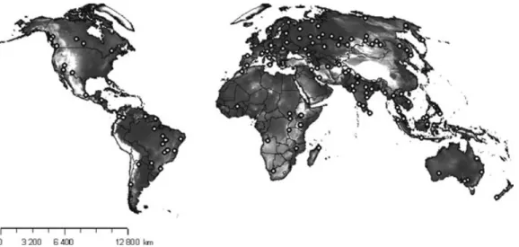
Figure 1. The 114 protected areas included in this study overlaid on the SRTM (Shuttle Radar Topography Mission) world digital elevation model (Supporting Information). Elevation ranges from a minimum of –418 m below sea level (black) to a maximum of 8682 m above sea level (white).
in the log-normalized size frequency distribution of all terrestrial protected areas in the WDPA database, so it represents the most common of the larger protected ar-eas worldwide. Second, we selected only terrestrial pro-tected areas in IUCN categories I–V. Category VI areas were excluded because they allow continual resource extraction within their borders, which we assumed re-sults in patterns of vegetation cover similar to that in the surrounding lands. Third, we eliminated protected areas with 10-20 km buffers that overlapped coastlines or in-cluded large water bodies. We did not want factors un-related to land cover (e.g., large areas of uniform surface water) to affect our measure of vegetation-cover hetero-geneity outside protected areas. Fourth, we eliminated protected areas that were part of reserve networks or that shared borders with other protected areas. Here, we did not want other protected areas to influence our mea-sure of vegetation-cover heterogeneity within 20 km of the protected-area border. Our sample was 114 protected areas, which represented 18% of all protected areas in the selected size range (Fig. 1; Supporting Information).
NDVI Values
The NDVI is an index of vegetation cover. It correlates directly with vegetation productivity, and mean NDVI is positively related to species richness (this relation is documented for a wide variety of plant types and animal populations) over large spatial grain and geographic ex-tent (Kerr et al. 2001; Hurlbert & Haskell 2003; Gillespie et al. 2008). Although species richness is positively re-lated to mean NDVI over large areas, it is often negatively related to NDVI variance at regional and continental ex-tents (Gillespie 2005; Levin et al. 2007; Rowhani et al. 2008). Carrara and V´azquez (2010) recently showed that the geographic distribution of bird and mammal species
richness across the Americas is best explained by the mean (positive relation) and variance (negative relation) of vegetation productivity measured as the actual evap-otranspiration per unit of surface area. In this context, the species-energy theory (Wright 1986) proposes that energy availability, or gross vegetation productivity, per unit of time and area regulates population sizes and thus species richness over large geographic areas (Carrara & V´azquez 2010).
We derived 12,32-day composite NDVI maps, 1 for each month of 2005, from the Moderate Resolution Imag-ing Spectroradiometer (MODIS, 500-m resolution) red (RED) and near-infrared (NIR) composite bands (NASA 2007). Values of NDVI are calculated as NIR− RED/NIR + RED (Tucker 1979). We demarcated 3 concentric, nonoverlapping buffers of 0–5 km, >5–10 km, and
>10–20 km from each protected-area border (hereafter
referred to as 0-5 km, 5-10 km, and 10-20 km buffers). A 10-20 km buffer around a protected area was deemed large enough to ensure we would identify any substantial variations in vegetation cover but proximal enough that changes in land-cover heterogeneity in the buffer likely influence population and ecosystem processes in the pro-tected area (Hansen & Defries 2007). We transformed the polygons and buffers of the protected areas into rasters and projected them on the MODIS NDVI maps. We ex-ported all geographic coordinates of pixels and associ-ated NDVI values to MATLAB (Matlab 2009) for analyses. We linearly rescaled the monthly NDVI values (R_NDVI) into 15 “greenness categories” as follows:
R NDVI= Ceil[15 ∗ (NDVI − MIN NDVI) / MAX NDVI], (1) where MIN_NDVI (alternatively, MAX_NDVI) is the low-est (highlow-est) NDVI value across all pixels of all sampled areas and buffers and Ceil is the MATLAB command
4 Protected-Area Isolation
for rounding to the nearest upper integer (zeros were rounded to R_NDVI = 1). Measured NDVI ranges (in parentheses) for the 15 greenness categories were G1 (<−0.49 to −0.40); G2 (−0.39 to −0.30); G3 (−0.29 to −0.20); G4 (−0.19 to −0.10); G5 (−0.09 to 0.00); G6 (0.01 to 0.10); G7 (0.11 to 0.20); G8 (0.21 to 0.30); G9 (0.31 to 0.40); G10 (0.41 to 0.50); G11 (0.51 to 0.60); G12 (0.61 to 0.70); G13 (0.71 to 0.80); G14 (0.81 to 0.90); G15 (0.91 to 1.00). Measuring Isolation
We estimated protected area isolation as the difference in contagion of NDVI values within each protected area and the contagion of NDVI values in concentric buffers around it. Positive values of this difference indicate higher land-cover heterogeneity (lower contagion of NDVI val-ues) (Proulx & Fahrig 2010) in the buffer surrounding the protected area than within its border.
Contagion is high (maximum contagion= 1) if there are few NDVI greenness categories and the land cover is distributed uniformly in space and time (i.e., large or single patches; low heterogeneity), whereas contagion is low (minimum contagion= 0) if land cover includes all 15 NDVI greenness categories and the pattern is ran-domly distributed in space and time (i.e., small and frag-mented patches; high heterogeneity). By using monthly NDVI maps, representing NDVI values for each month of 2005, we measured not only the spatial heterogene-ity, but also the within-year temporal heterogeneity. For example, protected-area isolation could result from dif-ferent seasonal dynamics in the land cover inside versus outside protected areas, such as when an area is domi-nated by evergreen forest (high temporal contagion in-side) but embedded in a matrix dominated by intensive agriculture, where greenness is more variable throughout the year (low temporal contagion outside). We calculated contagion with MATLAB codes written by R.P. for quanti-fying heterogeneity of the vegetation cover in space and time (Parrott et al. 2008).
We obtained a distribution of contagion values within each protected area and within each concentric buffer by using a moving-window procedure. Each window was a 3.5 km× 3.5 km × 12 month space-time cube of 588 pixels (i.e., 7× 7 × 12 = 588 pixels; each pixel was 500× 500 m) and was iteratively centered on a subset of pixels inside and outside the protected area (see boot-strap procedure below). We then calculated the mean contagion for each protected area and for each of its 3 buffers. The mean contagion of the 3 nonoverlapping buffers was then subtracted, separately, from the mean contagion inside the protected area. This produced, for each protected area, 3 measures of isolation at increasing distances from the border. Protected-area isolation was therefore positive when the mean contagion of NDVI values inside the protected area was higher (less
hetero-geneous) than outside its border and negative when the mean contagion of NDVI values inside the protected area was lower (more heterogeneous) than outside.
Given the large sample size (number of pixels) inside and outside protected areas, we used a bootstrap pro-cedure to estimate the uncertainty associated with our measure of protected area isolation. We resampled a sub-set of contagion values inside and outside protected areas without replacement (Molinaro et al. 2005) to account for the irregular, often multimodal distribution of contagion values across the landscape. With this procedure, we ob-tained the mean contagion inside and outside from equal sample sizes and independent bootstrap samples (i.e., re-peated samples do not share pixels) and ensured that the confidence intervals did not generate inflated type I error rates. For each combination of protected area and buffer zone, we repeated the bootstrap procedure 1000 times for a random subset of 100 windows inside and outside protected areas. We recorded the mean conta-gion difference and 95% confidence intervals (CI) as our measure of protected-area isolation. The isolation of an area was considered statistically significant if the 95% CIs of the inside-outside differences in mean contagion ex-cluded zero and if the effect size (i.e., the protected-area isolation) was≥0.05.
Explanatory Variables
We considered 4 variables that affect protected-area iso-lation. Two characterized land cover outside protected areas: elevation and human appropriation of net primary productivity (HANPP). For elevation we obtained a mea-sure of elevational difference between the protected area and the buffers because protected areas may often be at high elevations or have high topographic complex-ity (Scott et al. 2001; Hansen & Rotella 2002; Hansen & DeFries 2007). We extracted the elevations within each protected area and surrounding buffers from the Shuttle Radar Topography Mission (SRTM) 90-m Digital Elevation Model (Jarvis et al. 2008). We calculated el-evational difference as the maximum elevation within each protected area minus the minimum elevation within the 0-20 km buffer. These values of maximum and min-imum elevation were comparable with elevations re-ported in the WPDA data set for a number of protected areas.
For HANPP we obtained the percentage of HANPP (data taken from Imhoff et al. [2004]) as a measure of the land-cover alteration and human land-use intensity in the 5 nearest grid cells surrounding (and including) the longitude-latitude centroid of the protected areas (Sup-porting Information). For each 0.25◦grid cell of the world landmasses, percent HANPP is an estimate of the relative percentage of carbon from that area that is being used to derive food and fiber products consumed by humans on a per capita basis (Imhoff et al. 2004). As such, HANPP
is an index of the human footprint on each land grid cell (i.e., land-cover alteration, human population density and land-use intensity). Percent HANPP was assigned to the surrounding lands because protected areas were small (approximately 60,000 ha) relative to the summed area of the 5 nearest grid cells, which typically covered a surface area of about 6 times the protected area (approximately 378,000 ha at the equator).
The remaining 2 variables of protected area isolation characterized land cover inside protected areas: IUCN protection-status category and the variance in vegetation productivity (CV-NDVI) inside the protected area. We used the IUCN category of a protected area as an in-verse measure of its protection status. Protected areas in categories I–III effectively prevent human activity (e.g., land clearing, logging, hunting, grazing of livestock) in-side protected-area borders (Bruner et al. 2001). Thus, we grouped protected areas into high-protection (IUCN categories I–III) and low-protection (IUCN categories IV and V) categories.
We calculated the coefficient of variation (CV) of greenness (NDVI) values inside each protected area as an inverse generic measure of species richness. The geo-graphic distribution of species richness at large extents is strongly positively related to mean NDVI and negatively related to NDVI variance (e.g., Gillespie 2005; Levin et al. 2007; Rowhani et al. 2008). The CV-NDVI ratio quanti-fies the variance in vegetation productivity in time and space over a protected area (i.e., SD of all NDVI values inside its border) divided by its average vegetation pro-ductivity (i.e., mean of all NDVI values inside its border). Therefore, we assumed a low CV-NDVI ratio was indica-tive globally of landscapes that may have relaindica-tively high species richness. Although species richness may be asso-ciated indirectly with protected-area isolation, we think
it is important to examine whether protected areas that may have high species richness (lower CV-NDVI) are more isolated than areas in which species richness may be relatively low (higher CV-NDVI).
Statistical Analyses
Including the above 4 variables (i.e., elevation difference, percent HANPP, protection status, CV-NDVI), we fitted a regression model to the isolation values of our 114 protected areas. For protection status, we used a binary dummy variable that represented our high-protection cat-egory (IUCN categories I–III) versus low-protection cate-gory (IUCN categories IV and V). We fitted a separate re-gression model for each of the 3 buffers. We based model selection on all subsets following Sheather (2009) and the adjusted coefficient of determination (R2adj). To assess whether spatial autocorrelation in model residuals could bias statistical testing or indicate potential missing vari-ables (Peres-Neto & Legendre 2010), we calculated global Moran’s I autocorrelation coefficient for model residuals (Table 1) and tested for autocorrelation in residuals at dif-ferent spatial scales with correlograms (not shown here). We log transformed all noncategorical predictor variables to improve multinormality and stabilize variances. Visual inspection of normal probability plots (Q–Q plot) indi-cated model residuals were nearly normal. The pairwise correlation matrix among explanatory variables indicated colinearity was typically low (all Pearson’s r<0.25).
Results
Protected-area isolation from lands within both 0- to 5-km and 5- to 10-km buffers (hereafter, e.g., 0–5 km buffer)
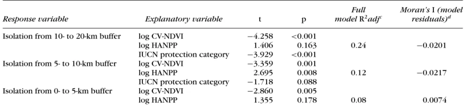
Table 1. Best regression modelsaof isolation of protected areas from concentric buffers at decreasing distances from the protected area (10–20 km, 5–10 km, and 0–5 km)b.
Full Moran’s I (model
Response variable Explanatory variable t p model R2adjc residuals)d
Isolation from 10- to 20-km buffer log CV-NDVI −4.258 <0.001
log HANPP 1.406 0.163 0.24 −0.0201
IUCN protection category −3.929 <0.001 Isolation from 5- to 10-km buffer log CV-NDVI −3.359 0.001
log HANPP 2.695 0.008 0.12 −0.0217
IUCN protection category −1.718 0.088
Isolation from 0- to 5-km buffer log CV-NDVI −2.860 0.005
log HANPP 1.355 0.178 0.08 0.0074
aModel selection was based on the coefficient of variation (CV) of the normalized difference vegetation index (NDVI) inside protected areas
(CV-NDVI), the percent human appropriation of net primary productivity (% HANPP) outside protected areas, and the IUCN protection category (low, [IUCN protection status IV-V] or high [IUCN protection status I-III]) of an area.
bA separate regression model is reported for each of the 3 nonoverlapping buffers (0–5 km,>5–10 km, and >10–20 km from each protected
area border) that were used to calculate isolation (i.e., the difference in contagion of NDVI values within each protected area and the contagion of NDVI values in each buffer).
cAdjusted coefficient of determination.
dGlobal Moran’s I autocorrelation coefficient for model residuals indicate residuals are not spatially patterned. This statistical approach is
described in Peres-Neto and Legendre (2010) and is based on the idea that the spatial relations among data points can be translated into explanatory variables that capture spatial effects at different spatial scales.
6 Protected-Area Isolation
Figure 2. Relation between protected area (PA) isolation, measured as the difference between mean contagion inside and in 3 nonoverlapping buffers outside each protected area, and the coefficient of variation of the normalized difference vegetation index (CV-NDVI); open circles and uppermost black line, 10- to 20-km buffer; black circles and black line, 5- to 10-km buffer; gray circles and gray line, 0- to 5-km buffer.
varied across the protected areas and included positive and negative values of isolation (Supporting Information). In contrast, isolation measured as the difference between mean contagion inside the protected area and in the 10-20 km buffer was strongly positive and was always higher than when it was measured as the difference between mean contagion inside the protected area and in the 0-5 km or 0-5-10 km buffers (Fig. 2 & Supporting Informa-tion). Values of protected-area isolation had high positive correlations between the values calculated on the basis of the 3 different buffers (isolation 10–20 km versus 5– 10 km, r2= 0.69, p < 0.001; isolation 5–10 km versus
0–5 km, r2= 0.89, p < 0.001).
Protected areas with a lower CV-NDVI ratio (more uni-formly green) inside their border tended to have higher isolation values (Fig. 2). Percent HANPP was positively as-sociated with protected-area isolation calculated on the basis of the 5-10 km and 10-20 km buffers (Table 1& Fig. 3). Isolation of protected areas in the high-protection category was significantly higher than isolation of pro-tected areas in the low-protection category (Fig. 3).
Elevational difference and protected-area isolation were not significantly related (Table 1). Nevertheless, areas in the high-protection category were generally lo-cated in regions of higher elevation than areas in the
Figure 3. Relation between protected area (PA) isolation, measured as the difference between mean contagion inside and in 2 nonoverlapping buffers outside each protected area, and the percent human appropriation of net primary productivity (HANPP): (a) 10- to 20-km buffer (low-protection category,
n= 60, r2= 0.11; p = 0.011) and (b) 5- to 10-km
buffer (low-protection category, r2= 0.07; p = 0.041). Areas are grouped by protection category (high, International Union for Conservation of Nature [IUCN] protection status I-III; low, IUCN protection status IV-V). The regression lines indicate significant relations obtained from bivariate linear models.
low-protection category (high protection maximum el-evation: mean [SE] = 1648 m [180]; low protection maximum elevation: mean = 1134 m [134], t = 2.286,
p= 0.0223), so the association between elevational
differ-ence and isolation may have been masked by the relation between protection category and isolation. There was no significant spatial autocorrelation in residuals for any of the 3 models produced (Table 1).
Discussion
The majority of protected areas were isolated from lands in the 20 km buffer. Vegetation cover in the 10-20 km buffer was more heterogeneous—contained more greenness categories distributed in smaller patches (more fragmented)—than the vegetation cover in the protected areas. Isolation, measured here by the difference in mean contagion, increased as the distance from the protected area border increased (up to 20 km), which suggests that human alteration of the vegetation cover pattern is less intense close to protected.
Our contagion measure, which we based on NDVI, expands on previous work in which protected-area iso-lation was quantified (e.g., DeFries et al. 2005; Joppa et al. 2008). Authors of these studies propose isolation measures be based on a binary [1,0] classification of tree cover. Such measures are only applicable to forest-or woodland-dominated ecosystems. Because contagion is independent of land-cover type, our isolation mea-sure remains comparable across different ecosystems. Measures of spatial and seasonal land-cover heterogene-ity have the potential to characterize the state of a protected area beyond simply the management of the ecosystem components inside its borders, and the land-cover matrix surrounding protected areas is crucial to achieving conservation goals (Franklin & Lindenmayer 2009).
We did not examine protected areas surrounded by other reserves. This selection criterion may have biased our sample toward more isolated protected areas. For ex-ample, Joppa et al. (2008) pointed out that in the African Congo and Amazon Basin, protected areas were often established in reserve networks and thus the vegetation pattern was similar inside and outside their borders. In re-gions where protected areas are not surrounded by other reserves, however, the results of our work are similar to those of Joppa et al. (2008) and DeFries et al. (2005), that is, vegetation cover in lands surrounding the majority of protected areas is measurably, and increasingly, differ-ent (i.e., more heterogeneous or fragmdiffer-ented) from the surrounding land-cover matrix.
All covariates but elevational difference explained a significant part of the variance in protected-area isolation when considering at least 1 of any 3 buffer zones. Nev-ertheless, our best statistical model explained only 24% of the overall variance in protected-area isolation, and a large part of the variance was explained by one vari-able (CV-NDVI). The negative relation of CV-NDVI with isolation suggests that protected areas with land cover that, relative to other regions, is uniformly greener may be more likely to be isolated. This means protected ar-eas in different regions of the world can have different likelihoods of relative isolation. Lowland regions covered by evergreen forests (i.e., lower CV-NDVI) may be more likely to be isolated than other vegetation types. For
in-stance, among the 5 protected areas with the highest isolation from buffers at 10–20 km, 4 were in tropical forests (Supporting Information). Because higher mean and lower variance in vegetation productivity over a land-scape may be related to higher species richness (e.g., Carrara & V´azquez 2010), higher probability of isolation among the world’s greener protected areas (with low CV-NDVI ratios) may also suggest a higher probability of species extinctions or extirpations outside and extir-pation inside these areas. Hence, independent of other anthropogenic drivers of isolation, protected areas with high species richness and endemism (e.g., tropical forest) may also be the most likely to be isolated (or have high levels of isolation) from surrounding areas.
Variables other than the 4 we tested may be respon-sible for the 76% of unexplained variation in protected-area isolation. Such variables are likely to be related to regional variation in contagion due to hydrology and topography and to specific human land uses, such as agriculture and urbanization. For example, increased vegetation-cover heterogeneity associated with the pres-ence of a river system or with various agricultural and forestry uses (e.g., plantations, logging, crops, or live-stock grazing) may not be captured well by our aggregate measures of elevational difference and percent HANPP. Nevertheless, a more detailed understanding of the en-vironmental, social, and economic processes associated with protected area isolation will probably not be easily applicable across the global network of protected areas. Isolation of protected areas in the high-protection gory was high relative to areas in the low-protection cate-gory. All else being equal, this suggests protected areas in the high-protection category are effective at maintaining the pattern of vegetation-cover heterogeneity, whereas vegetation cover of the surrounding lands is fragmented by human activity. Alternatively, the relatively high iso-lation of areas in the high-protection category could be due to the fact that these areas tended to be at higher elevations. Although we confirmed this possibility in the high-protection versus low-protection categories, we also found that elevational difference (maximum elevation in-side versus minimum elevation outin-side) was not asso-ciated with our measure of isolation. Therefore, it is not clear whether elevation is a factor in the relation between protection area status and isolation.
A prominent issue in recent research has been whether the establishment of a protected area encourages human settlement and population growth or whether protec-tion deters settlement and land use beyond the borders of a protected area (Wittemyer et al. 2008; Joppa et al. 2009). Joppa et al. (2009) recently argued that population growth near the borders of protected areas results from a general expansion of nearby human populations. Hu-man activities that alter land cover and isolate protected areas may spread toward the protected area over time. This might explain why we found a stronger relation
8 Protected-Area Isolation
between percent HANPP and isolation among areas in the low-protection category; such areas are typically placed closer to centers of intensive human activities (Hansen & Rotella 2002). Our results suggest that areas in the low-protection category had lower isolation values than areas in the high-protection category because vegetation in the protected area was not preserved, yet the degree of isola-tion in low-protecisola-tion areas still appears directly affected by human activities in the surrounding lands.
Our results, and those of others, suggest the IUCN pro-tection status of an area is associated with the extent to which a protected area has been maintained in a state that is relatively unaffected by human activities (i.e., its “natural” state). Despite their effectiveness in this sense, our results also indicate that even protected areas in high-protection categories are becoming increasingly isolated in the sense that they are increasingly unrepresentative of the ecological region they are meant to represent. Our results therefore add to the growing recognition that conservation of species and ecosystems cannot be ac-complished solely through the establishment and man-agement of protected areas.
Acknowledgments
Financial support to I.S. was provided by the Natural Sciences and Engineering Research Council of Canada (NSERC) for this work. We thank M. Desrochers for her technical support, contributions, and valuable com-ments. We are grateful to 2 anonymous reviewers and the editors for their helpful comments. MATLAB source code used to calculate the contagion metric described here can be obtained by contacting R.P.
Supporting Information
The complete data set for the 114 protected areas (Ap-pendix 1S) is available online. The authors are solely re-sponsible for the content and functionality of this mate-rial. Queries (other than absence of the material) should be directed to the corresponding author.
Literature Cited
Bruner, A. G., R. E. Gullison, R. E. Rice, and G. A. B. da Fonseca. 2001. Effectiveness of parks in protecting tropical biodiversity. Science
291:125–128.
Carrara, R., and D. P. V´azquez. 2010. The species-energy theory: a role for energy variability. Ecography33:942–948.
DeFries, R., A. Hansen, A. C. Newton, and M. C. Hansen. 2005. In-creasing isolation of protected areas in tropical forests over the past twenty years. Ecological Applications15:19–26.
DeFries, R., A. Hansen, B. L. Turner, R. Reid, and J. Liu. 2007. Land use change around protected areas: management to bal-ance human needs and ecological function. Ecological Applications
17:1031–1038.
Franklin, J. F., and D. B. Lindenmayer. 2009. Importance of matrix habi-tats in maintaining biological diversity. Proceedings of the National Academy of Sciences106:349–350.
Gillespie, T. W. 2005. Predicting woody-plant species richness in trop-ical dry forests: a case study from South Florida, USA. Ecologtrop-ical Application15:27–37.
Gillespie, T. W., G. M. Foody, D. Rocchini, A. P. Giorgi, and S. Saatchi. 2008. Measuring and modelling biodiversity from space. Progress in Physical Geography32:203–221.
Hansen, A. J., and J. J. Rotella. 2002. Biophysical factors, land use, and species viability in and around nature reserves. Conservation Biology16:1112–1122.
Hansen, A. J., and R. DeFries. 2007. Ecological mechanisms link-ing protected areas to surroundlink-ing lands. Ecological Applications
17:974–988.
Hurlbert, A. H., and J. P. Haskell. 2003. The effect of energy and season-ality on avian species richness and community composition. The American Naturalist161:83–97.
Imhoff, Marc L., L. Bounoua, T. Ricketts, C. Loucks, R. Harriss, and W. T. Lawrence. 2004. Human appropriation of net primary productivity (HANPP). Socioeconomic Data and Applications Center (SEDAC), Columbia University, New York. Available from http://sedac.ciesin. columbia.edu/es/hanpp.html (accessed June 2008).
Jarvis, A., H. I. Reuter, A. Nelson, and E. Guevara. 2008. Hole-filled seamless SRTM data V4. International Centre for Tropical Agricul-ture (CIAT), Cali, Columbia.
Joppa, L. N., S. R. Loarie, and S. L. Pimm. 2008. On the protection of “protected areas.” Proceedings of the National Academy of Sciences of the United States of America105:6673–6678.
Joppa, L. N., S. R. Loarie, and S. L. Pimm. 2009. On population growth near protected areas. Public Library of Science ONE 4 DOI:10.1371/journal.pone.0004279.
Karr, J. R., and D. R. Dudley. 1981. Ecological perspective on water quality goals. Environmental Management5:55–68.
Kerr, J. T., T. R. E. Southwood, and J. Cihlar. 2001. Remotely sensed habitat diversity predicts butterfly species richness and community similarity in Canada. Proceedings of the National Academy of Sciences of the United States of America 98:11365–
11370.
Levin, N., A. Shmida, O. Levanoni, H. Tamari, and S. Kark. 2007. Pre-dicting mountain plant richness and rarity from space using satellite-derived vegetation indices. Diversity and Distributions 13:692– 703.
Li, H., and J. F. Reynolds. 1993. A new contagion index to quantify spatial patterns of landscapes. Landscape Ecology8:155–162. Matlab. 2009. MathWorks. Matlab, Natick, Massachusetts.
Molinaro, A. M., R. Simon, and R. M. Pfeiffer. 2005. Prediction error estimation: a comparison of resampling methods. Bioinformatics
21:3301–3307.
NASA (National Aeronautics and Space Administration). 2007. MODIS 16-day composite MOD44C, latlon.na.2004289b3. Collection 4. The Global land cover facility, University of Maryland, College Park. Newmark, W. D. 2008. Isolation of African protected areas. Frontiers
in Ecology and the Environment6:321–328.
O’Neill, R. V., et al. 1988. Indices of landscape pattern. Landscape Ecology1:153–162.
Parks, S. A., and A. H. Harcourt. 2002. Reserve size, local human density, and mammalian extinctions in U.S. protected areas. Conservation Biology16:800–808.
Parrott, L., R. Proulx, and X. Thibert-Plante. 2008. Three-dimensional metrics for the analysis of spatiotemporal data in ecology. Ecological Informatics3:343–353.
Peres-Neto, P. R., and P. Legendre. 2010. Estimating and controlling for spatial autocorrelation in the study of ecological communities. Global Ecology and Biogeography19:174–184.
Peres, C. A. 2005. Why we need mega-reserves in Amazonia. Conserva-tion Biology19:728–733.
Proulx, R., and L. Fahrig. 2010. Detecting human-driven deviations from trajectories in landscape composition and configuration. Landscape Ecology25:1479–1487.
Rowhani, P., C. A. Lepczyk, M. A. Linderman, A. M. Pidgeon, V. C. Radeloff, P. D. Culbert, and E. F. Lambin. 2008. Variability in energy influences avian distribution patterns across the USA. Ecosystems
11:854–867.
Scott, J. M., F. W. Davis, R. G. McGhie, R. G. Wright, C. Groves, and J. Estes. 2001. Nature reserves: do they capture the full range of America’s biological diversity? Ecological Applications11:999– 1007.
Sheather, S. J. 2009. A modern approach to regression with R. Springer-Verlag, New York.
Tucker, C. J. 1979. Red and photographic infrared linear combina-tions for monitoring vegetation. Remote Sensing of Environment
8:127–150.
UNEP (United Nations Environment Programme). 2009. The World database on protected areas (WDPA). UNEP-WCMC (World Con-servation Monitoring Centre), Cambridge, United Kingdom. Wittemyer, G., P. Elsen, W. T. Bean, A. C. O. Burton, and J. S. Brashares.
2008. Accelerated human population growth at protected area edges. Science321:123–126.
Woodroffe, R., and J. R. Ginsberg. 1998. Edge effects and the extinction of populations inside protected areas. Science280:2126–2128. Wright, D. H. 1986. Species-energy theory: an extension of species-area